Light diffuseness metric,Part 2: Describing,measuring and visualising the light flow and diffuseness in three-dimensional spaces

Abstract

We introduce a way to simultaneously measure the light density, light vector and diffuseness of the light field using a cubic illumination meter based on the spherical harmonics representation of the light field. This approach was applied to six light probe images of natural scenes and four real scenes built in our laboratory, and the results were compared to those obtained using Cuttle’s method. We also demonstrated a way to simultaneously and intuitively visualise the global structure of the light distribution using light tubes and colour coding for the light density, light flow and diffuseness variations through the space. Together with Mury’s work, we have a complete way to describe, measure and visualise the local and global low-order properties of light distributions in three-dimensional spaces.

1. Introduction

The distribution of light in a three-dimensional space strongly influences the appearance of that space and the objects inside it. There is no doubt that the primary purpose of artificial lighting is pure visibility. However, with advances in lighting technology, peoples’ expectation of lighting now far exceeds this primary function. Modern designers prefer to see lighting principally in terms of how it influences the appearance of people’s surroundings and makes it possible to create various atmospheres.^1–6 In this line of thought, Cuttle⁷ proposed that the lighting profession must move to the third stage. The first stage of the lighting profession focused on providing uniform illumination over a horizontal plane, whereas the second stage provided illumination suited to human needs based on visual performance. Cuttle stated that the third stage should aim at revealing the potential of illumination to interact with its surroundings to create various types of visual experiences. In order to do so, we require methods to describe, measure and visualise the structure of the light distribution throughout the space. These methods provide insights into the spatial and form-giving character of light and allow predictions of how an object would appear in this light. In this paper, we introduce ways to measure the physical (objective) light diffuseness. The (subjective) perception of light diffuseness is influenced by many additional factors such as the illumination direction,^8,9 the shape and material of the illuminated object and the perspective of the observer.¹⁰ Relating perceptual diffuseness ratings to systematic variations of the physical diffuseness thus encompasses an extensive psychophysical study, which we intend to do in the future.

The light density, the primary illumination direction, and the diffuseness shapes the basic (low-order) properties of a light field, which can be sensed by the human visual system.^8,11–13 The light density and direction were mathematically and physically defined by Gershun¹⁴ in his five-dimensional function of the light field and by Mury¹⁵ using a spherical harmonics (SH) representation of the light field. In Part 1 of this work, we gave a review of four well-known diffuseness metrics, namely (1) the ‘scale of light’ by Frandsen¹⁶ (D_Frandsen), (2) the ‘ratio between cylindrical and horizontal illuminance’ by Hewitt et al.¹⁷ (D_Hewitt), (3) the ‘ratio between illumination vector and scalar’ by Cuttle⁹ (D_Cuttle) and Lynes et al.¹⁸ and (4) the ‘Illuminance Contrast Energy (ICE)’ metric of Morgenstern et al.¹⁹ (D_Morgenstern). Their relationships were examined via a model named ‘probe in a sphere’ and the results showed that the normalised diffuseness metrics D_Hewitt, D_Cuttle and D_Morgenstern gave very similar results to the ‘probe in a sphere model’. Inspired by Mury’s work on the physical SH representation of the light field and by the basic parameterisation of diffuseness as the balance between the ambient and directed light, we proved that D_Cuttle is equivalent to the ratio between the strength of the first order (i.e. the light vector) and the zeroth order (i.e. the light density) of the SH representation of the light field (D_Xia). The diffuseness metric D_Xia is entirely based on a mathematical description of the physical light distribution and fulfils the criteria we defined as being relevant for a diffuseness metric. Together with the light density and direction, it represents the low-order properties of the global structure of the light field. Furthermore, the SH-based method allows all parameters to be described within one integral description/decomposition, in which it is clear how the parameters relate and which role they play in the resulting light field. For instance, Kelly,^1,2 considered to be one of the pioneers of architectural lighting design, used ‘ambient luminescence’, ‘focal glow’ and ‘play of brilliants’ to describe the light effects in lighting design. In the SH representation of the light field, the zeroth order describes the ‘ambient luminescence’, the first order gives information about ‘focal glow’ and the higher orders are related to the ‘play of brilliants’.

In this study, we demonstrate how the density of light, light direction and diffuseness can be simultaneously measured using a cubic illumination meter and visualised using ‘light tubes’.

2. Measuring the light field’s light density, direction and diffuseness simultaneously

2.1. Cuttle’s method

Cuttle proposed a simple solution to measure the illumination vector and scalar, as well as the ratio between illumination vector and scalar (i.e. the inverse of the light diffuseness).^20,21 Using a cubic illumination meter, six illuminance values in three mutually perpendicular directions can be measured, these being E₍ _+x ₎, E₍ _−x ₎, E₍ _+y ₎, E₍ _−y ₎, E₍ _+z ₎, E₍ _−z ₎. The illumination vector component can be calculated as

E vector = (E (+ x) - E (- x), E (+ y) - E (- y), E (+ z) - E (- z))

(1)

and the scalar component as

E scalar = | E vector | 4 + \bar{E} symmetric = | E vector | 4 + {min (E (+ x), E (- x)) + min (E (+ y), E (- y)) + min (E (+ z), E (- z))} 3

(2)

with ‘min’ denoting the minimum. Consequently, the strength of the flow of light (i.e. the inverse of the light diffuseness) can be easily found as | E_vector |/E_scalar. The normalised form of the diffuseness is

(D Cuttle) Normalized = 1 - (| E vector | / E scalar) / 4

(3)

with ‘0’ corresponding to fully collimated light and ‘1’ corresponding to fully diffuse light. Cuttle’s method uses simple calculations and is suitable for quick, local measurements of the diffuseness level of natural scenes.

2.2. Xia’s method

In this section, we propose a similar but differently framed approach to simultaneously recover these main, low-order properties of the light field using a SH representation of the light field. In Part 1 of this work (light diffuseness metric Part 1: Theory), we proved that the ratio between the strength of the first-and zeroth-order components of the SH representation (D_Xia) gives the diffuseness. Thus, to simultaneously measure the light density, direction and diffuseness, the first two orders of the SH representation of the light field are sufficient.

Mury et al.²² managed to measure the light field up to the second-order SH representation by using a custom-made device called a ‘Plenopter’. This second-order representation consists of nine coefficients, which could be estimated using a device composed of 12 faces with a light sensor on each. Since we only need the zeroth and first order of the representation, we only need to estimate four coefficients, which can be done with a cubic illumination meter.

The cubic illumination meter comprises six illuminance meters mounted on the faces of a small cube, yielding six values P_j (j = 1,…, 6). The illuminance meters have a certain angular sensitivity profile S_j (ϑ, ϕ) that should be convoluted with the incident light distribution f_j (ϑ, ϕ) on that illuminance meter. Thus

P j = \int S j (ϑ, ϕ) \cdot f j (ϑ, ϕ) d Ω j = 1, \dots, 6

(4)

The illumination meter’s angular sensitivity profile can be decomposed to SHs and presented as

S j (ϑ, ϕ) = \sum l = 0 \infty \sum m = - l l (s j) l m Y l m (ϑ, ϕ)

(5)

The shape of the sensitivity profile follows the cosine law as a function of the angle between the incident direction of light and the normal to the surface to which the meter is attached. Furthermore, the incident light can be reconstructed by the sum of its harmonics. Combining the above results in

P j = \int [\sum l = 0 \infty \sum m = - l l (s j) l m Y l m (ϑ, ϕ)] \times [\sum l' = 0 \infty \sum m' = - l' l' C l' m' Y l' m' (ϑ, ϕ)] d Ω = \sum ll' mm' (s j) l m C l' m' \int Y l m (ϑ, ϕ) Y l' m' (ϑ, ϕ) d Ω j = 1, \dots, 6

(6)

where

C l' m'

are the coefficients of the SH decomposition of the incident light filed.

Because of the orthonormality of the SH basis function, we finally get

P j = \sum lm (s j) l m C l m j = 1, \dots, 6

(7)

Thus, we obtain a system of six equations with four unknown coefficients. By using a least squares approach, solutions for the overdetermined system can be fitted. Thus, the zeroth- and first-order modes of the SH representation of the light field can be recovered and these carry the information about the light density (i.e. the zeroth order), the light vector (i.e. the first order) and the normalised diffuseness as

(D Xia) Normalized = 1 - d (L 1) / d (L 0) / \sqrt{3}

(8)

where d(L₀) is the strength of the zeroth order, and d(L₁) indicates the strength of the first-order SH representation of the light field. In the normalised diffuseness metric, ‘0’ corresponds to fully collimated light and ‘1’ corresponds to fully diffuse light. The advantages of the SH representation are that all parameters can be described within one integral description/decomposition, in which it is clear how the parameters relate and which role they play in the resulting light field. Moreover, the SH representation can be used as such in, for instance, fast real-time computer rendering and can be linked to components of lighting plans for design and architecture.

The cubic illumination meter is easily built with commercially available components, namely the Konica-Minolta T-10MA illuminance meters (as shown in Figure 1). Additional materials are provided in the Appendix for laser-cutting and building the cube base.

Figure 1.

Our cubic illumination meter, built with commercially available components on the basis of a laser-cut cube base (see Appendix for additional materials to build this base). Note: our cubic illumination meter has six large faces and two small faces. The small face on the top was cut to place a spirit level, and the small face on the bottom was cut to fix the cubic meter onto a metal stick.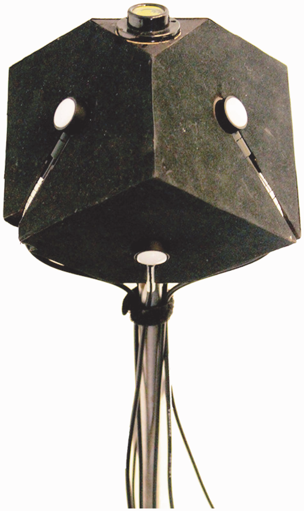

3. Measurement error predictions

3.1. Error analysis: Influence of light field orientation and second-order SH contributions

How robustly can D_Xia and D_Cuttle measure the diffuseness of a light field using a cubic illumination meter? To answer this question, we simulated a light field by using a sum of SH functions. According to Ramamoorthi and Hanrahan,²³ complex lighting on approximate Lambertian surfaces can be successfully replaced by its second-order approximation. Thus, we simulated a light field in terms of a second-order SH representation

We varied the ratios defining the relative strength of the first three orders (i.e. w₁/w₀, w₂/w₀) and the weights of the components within the first and second order (i.e. a₁, a₂, a₃; b₁, b₂, b₃, b₄, b₅). Since the theoretical value of d(L₁)/d(L₀) for the model ‘probe in a sphere’ ranges from 1.73 to 0, we set the range of w₁/w₀ from 0 to 1.7 with an interval of 0.1. We then calculated the theoretical illumination falling on the six faces of the cubic meter under the simulated light field. With these six values, we calculated D_Cuttle. Next, we used the least squares approach to fit the four coefficients of the zeroth- and first-order SH representation and determined D_Xia. The results are shown in Figures 2 and 3.

Figure 2.

Simulated diffuseness values as a function of the theoretical diffuseness for four different weight distributions within the first-order component. (a) D_Xia, (b)D_Cuttle.

Figure 3.

Simulated diffuseness values as a function of the theoretical diffuseness for two relative strengths of the second-order SH component w₂/w₀ (0.5 or 1). For w₂/w₀ = 1, two different weights distributions within the second-order components were adopted. The first-order components were set as a₁ = 0, a₂ = 1, a₃ = 0. (a) D_Xia, (b) D_Cuttle.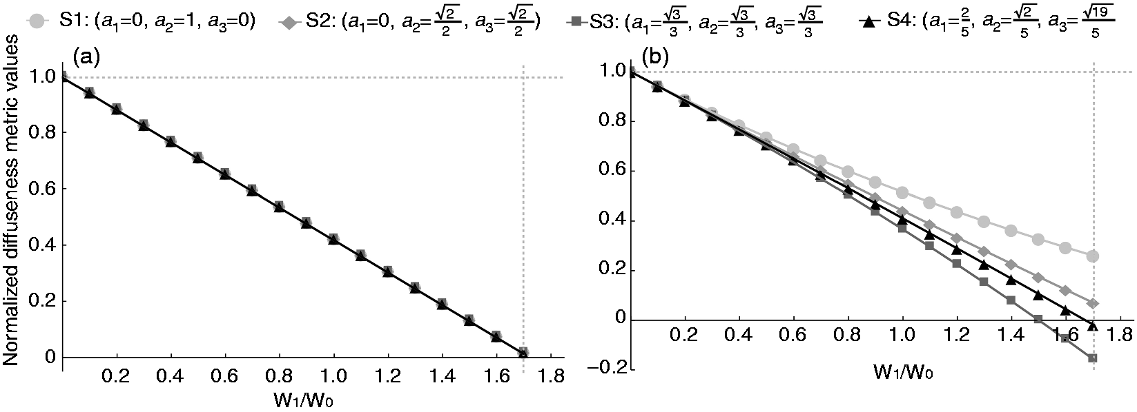

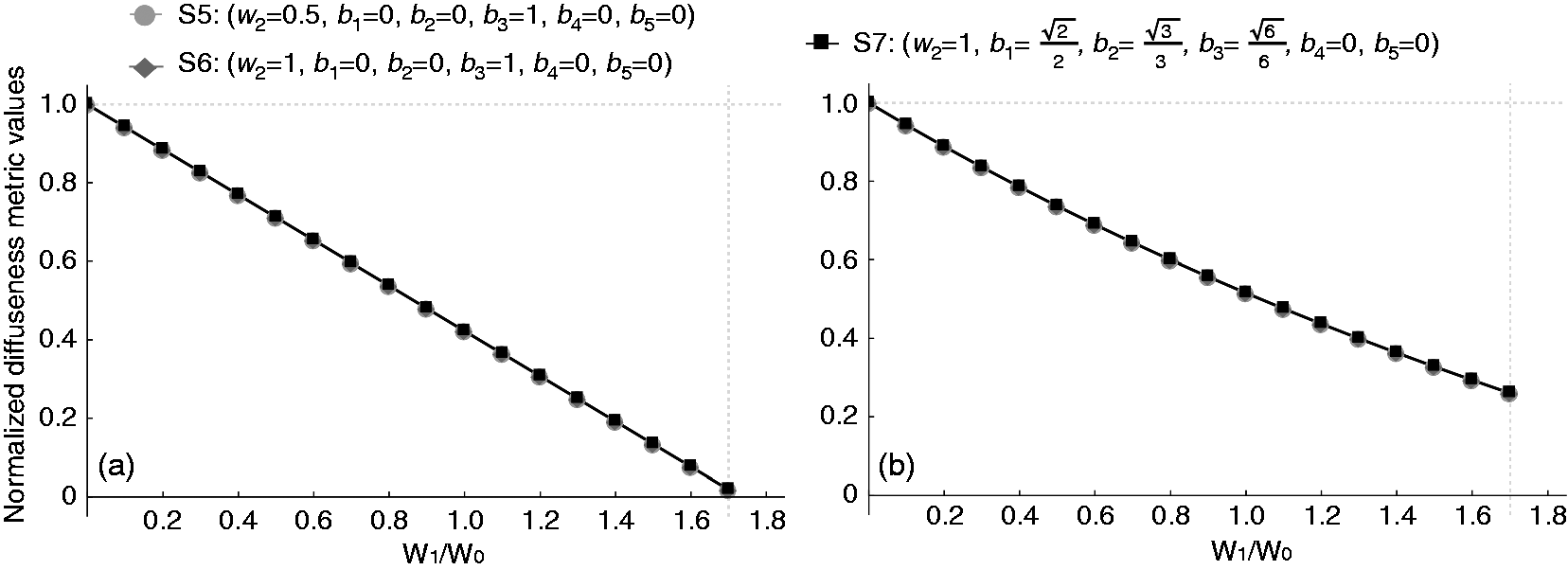
Figure 2 shows the normalised D_Xia and D_Cuttle values calculated as a function of the relative strength w₁/w₀ for different weights of the first-order components (i.e. a₁, a₂, a₃), representing different orientations of the light field, while its structure remains the same. Clearly, the straight line shows that the original D_Xia value (before normalisation) is exactly the same as w₁/w₀. D_Cuttle deviates from w₁/w₀ with a slope being dependent on the weights of the first-order components or the orientation of the light field.

Figure 3 shows the normalised D_Xia and D_Cuttle values as a function of w₁/w₀ for different relative strengths w₂/w₀ and weights of the second-order components (i.e. b₁, b₂, b₃, b₄, b₅). Both the calculated D_Xia and D_Cuttle are independent of w₂/w₀ and of the weights of the second-order components (the three curves in each plot overlap).

3.2. Error analysis: Effect of attitude of the cubic illumination meter

In Section 3.1, we found that D_Cuttle depended on the orientation of the light field. This implies that D_Cuttle will vary with the cubic illumination meter’s attitude in the light field. Here, we analyse this variation and evaluate whether optimising the meter’s attitude can reduce measurement errors.

In order to answer the question above, the model ‘probe in a sphere’ was used. We chose four different attitudes for the cubic illumination meter; their bird’s eye views are illustrated in Figure 4. In Figure 4(a), the cubic illumination meter was positioned symmetrically with respect to the light source with four faces parallel to the light vector along the z-axis. As a consequence, these four faces always received the same illumination (Attitude 1). Figure 4(b) shows Attitude 2, for which we rotated the cubic illumination meter 20° around the x-axis, so that it had two faces parallel to the light vector, receiving the same illumination. For Attitude 3, illustrated in Figure 4(c), we did an additional rotation of 15° around the y-axis, so that no faces were parallel to the light vector and all received a different amount of illumination. Finally, for Attitude 4, shown in Figure 4(d), the cubic illumination meter was first rotated 45° around the x-axis and then rotated 35° around the y-axis, so that one of the diagonals was parallel to the z-axis. As a consequence, it had no face parallel to the light vector, but the three faces turned upwards all received the same illumination, and the other three faces turned downwards did likewise. We then calculated the illumination falling on the six faces of the cubic illumination meter for the four attitudes and for subtended angles of the spherical light source ranging from 0° to 360°. For each situation, we fitted the four coefficients of the SH representation of the light field and used them to determine D_Xia. In Figure 5(a), we show the simulated and normalised D_Xia values together with the theoretical diffuseness values for the different subtended angles. The theoretical diffuseness values were obtained by fitting the SH representations to the luminance maps of our model instead of to the simulated cubic illumination meter readings.

Figure 4.

The simulated attitudes of the cubic illumination meter in the centre of the large spherical light source, with the light vector along the z-axis: (a) attitude 1: the cubic illumination meter was symmetrically positioned with respect to the light source with four faces parallel to the z-axis, (b) attitude 2: rotated 20° around the x-axis, (c) attitude 3: with an additional rotation of 15° around the y-axis, and (d) attitude 4: firstly rotated 45° around the x-axis and then rotated 35° around the y-axis.

Figure 5.

(a) Simulated D_X_ia values and (b) simulated D_C_uttle values, as a function of the subtended angle α of the spherical light source for four cubic illumination meter attitudes.

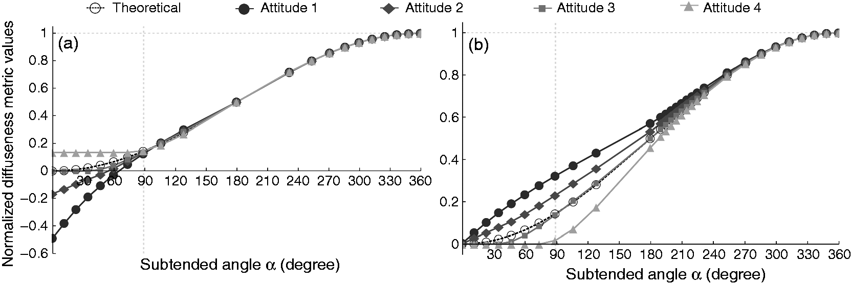
When the subtended angle α was bigger than 180°, all six faces of the cubic illumination meter were illuminated, and the recovered D_X_ia was exactly the same as the theoretical one. When α was larger than 90° but smaller than 180°, at least five faces of the cubic illumination meter were illuminated, and then the recovered D_X_ia was quite close to the theoretical one. When α was smaller than 90°; however, the recovered D_X_ia was different between the four attitudes, and only the curve for Attitude 3 was close to the theoretical value. So, D_X_ia approached the theoretical values best when the number of illuminated faces was maximised and diversified and is a logical result of the SH fitting procedure. This effect implies that D_X_ia is not robust for extremely collimated light if we put the cubic illumination meter symmetrically with respect to the light source. In such cases, the normalised D_X_ia may generate negative values (see Figure 5(a)). This happens because of the least squares fitting approach of the SH functions. When the light source is rather collimated (subtended angle <90°), some of the faces of the cubic illumination meter (e.g. the bottom face) may not be illuminated and set to zero in our fitting approach. However, the first-order SH representation of the light field varies rather symmetrically and smoothly over all directions. Consequently, a small part of the energy will be in the higher order terms of the SH fit, which is excluded from our analysis (analogous to what happens for a block wave or called ‘ringing’ effects in Fourier decompositions). Fortunately, this situation is quite uncommon in natural scenes because there are always reflections from surroundings in real lighting environments.

In Figure 5(b), we show the simulated and normalised D_C_uttle values together with the theoretical diffuseness. Consistent with the findings in Section 3.1, D_C_uttle varied with the attitude of the cubic illumination meter, though all curves originate in zero. Furthermore, the optimisation guidelines that apply to D_X_ia also apply to D_C_uttl_e.

4. Simulated cubic illumination measurements

In order to investigate the robustness of D_X_ia and D_C_uttle in real complicated lighting environments, we first simulated cubic illumination meter measurements. To do so, we employed six HDR panoramic light probe images from Debevec’s high-resolution light probe image gallery.^24,25 The images used were named ‘dining room’, ‘Uffizi gallery’, ‘Grace cathedral’, ‘Doge’s palace’, ‘sunset’ and ‘glacier’, and their gray-scale tone maps are shown in Figure 6.

Figure 6.

The grayscale tonemaps for HDR panorama photographs of six natural scenes (a) dining room (b) Uffizi gallery (c) Grace cathedral (d) Doge’s palace (e) sunset (f) glacier.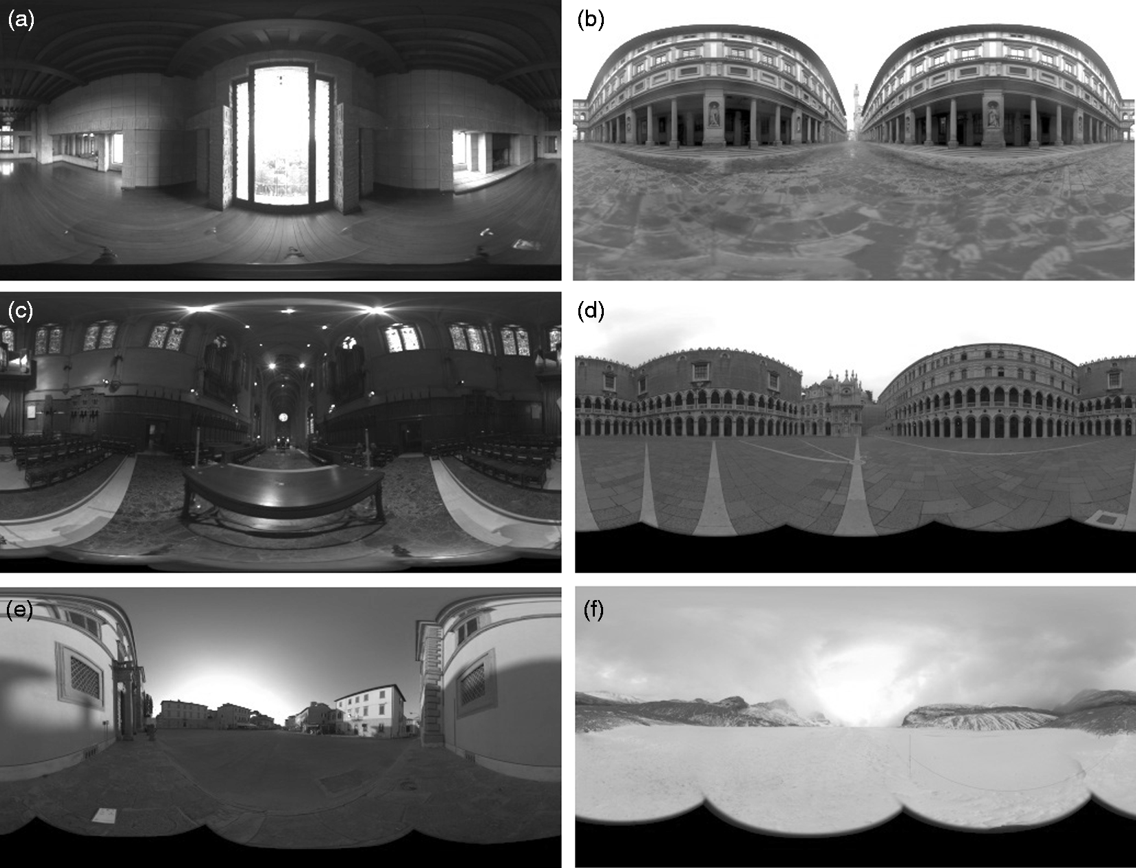

We assumed a cubic illumination meter right in the centre of each scene. Since the values recovered from this meter may be influenced by the cube orientation, we simulated one hundred attitudes of the meter for each light probe image, by systematically varying the latitude and longitude of the cube in 20° intervals. We then calculated the illuminance on the six faces of the meter for each attitude in each light probe image. From these illuminances, the normalised D_X_ia and D_C_uttle were calculated and plotted in Figure 7. The boxes with dashed frames in Figure 7 indicate the distribution of normalised D_C_uttle values, while the boxes with solid frames show the distribution of normalised D_X_ia values. The median value of all boxes is consistent with the value d(L₁)/d(L₀) that was calculated from the complete SH representation of each light probe image.

Figure 7.

Box plot for normalised D_C_uttle and D_X_ia values obtained from 100 different simulated attitudes of the cubic illumination meter in six light probe images. The black ‘*’ indicate the normalised d(L₁)/d(L₀) estimated from the full SH representation of each image.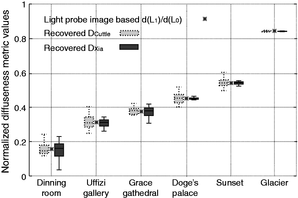

The recovered D_C_uttle values seem less sensitive to the cubic illumination meter’s orientation than the recovered D_X_ia values for the scenes ‘dining room’ and ‘Grace cathedral’, while the opposite is true for the other scenes. In Section 3.1, we prove that, in theory, the recovered D_X_ia reflects d(L₁)/d(L₀) well, while the recovered D_C_uttle is expected to vary with the orientation of the meter in the light field. However, in Section 3.2, we show that D_X_ia estimates are expected to vary somewhat in collimated light. In such light, the faces of the cube away from the collimated light source are not illuminated, and so, their values are set to zero; this hinders robust SH fitting. The scenes ‘dining room’ and ‘Grace cathedral’ have more small bright, collimated light sources than the other scenes, and so were expected to yield less robust results for D_X_i_a. Based on these findings, we conclude that the recovered D_C_uttle value is somewhat better at measuring light fields with a high contrast, such as in dark interior scenes with small bright windows or lamps, while the recovered D_X_ia metric is more suitable for light fields with low contrast, such as for open outside environments. However, overall, the D_C_uttle and D_X_ia simulations show only a small spread over the 100 different attitudes of the meter, which indicates that both of them can well be used to measure the diffuseness for any random orientation of the meter.

In a former study by Pont and Koenderink⁸, observers matched levels of diffuseness on spheres using a visual probe. These results showed that the perceived diffuseness correlated well with physical changes in the stimuli, but the variance was quite large. In another study by Xia et al.²⁶, observers were asked to judge whether a probe fitted a scene in terms of lighting for different settings of diffuseness on probe and scene. These results showed that the observers could not perceive a mismatch in diffuseness for small differences between probe and scene (i.e. for differences in scale of light between 24% and 43%, and between 43% and 59%). The latter values correspond to 0.01, 0.05 and 0.1 in normalised D_X_ia or D_C_uttle units, respectively. Thus, the errors in our simulated measurements are relatively small compared to typical spreads in perceived diffuseness.

5. Real cubic illumination measurements

In order to systematically vary the diffuseness in a real scene, we built a box space of two walls forming a corner, in which we varied the reflectance of the walls and the primary illumination source. The reflectance was changed by putting either white or black paper (i.e. photography background paper rolls, all 2 m wide and room-height) in front of these walls. The white matte environment was used to generate secondary reflections by diffuse scattering, and thus showed an increase in light density or ambient illumination, in comparison to the black environment. We illuminated the corner with a spotlight (i.e. collimated light) or by indirect illumination via the ceiling with two large diffuse lamps (i.e. semi-diffuse light from above). Thus, the two environments and two types of luminaires resulted in four different light fields in total (i.e. LF I: semi-diffuse light plus white background; LF II: collimated light plus white background; LF III: semi-diffuse light plus black background; LF IV: collimated light plus black background). The cubic illumination meter was put in the centre of the corner. Table 1, showing the resulting measurements, illustrates that the results were quite similar for the two approaches for all light fields. The diffuseness varied systematically for the light fields; the values for the spotlight were indeed lower than for the semi-diffuse light from above. Note that the environment reflectance had a much bigger impact on the light qualities than the luminaires; the diffuseness increased by about 0.6 if the black walls were changed into white ones.

Table 1.

The average illuminance, the light vector in Cartesian coordinates, and the normalised diffuseness level at the location of the meter in four different light fields for both Cuttle’s and Xia’s approach.

			Light vector
Method	Light field	E_average (lm/m²)	Unit light vector	Magnitude	Normalised diffuseness
Cuttle	I	240.3	(−0.36, 0.58, 0.73)	113.32	0.88
	II	950.7	(0.38, 0.77, 0.51)	669.58	0.82
	III	68.5	(0.56, 0.73, 0.38)	199.15	0.27
	IV	365.2	(0.68, 0.68, 0.25)	1221.20	0.14
Xia	I	235.9	(-0.36, 0.58, 0.73)	113.30	0.88
	II	972.9	(0.38, 0.77, 0.51)	669.49	0.83
	III	75.7	(0.56, 0.73, 0.38)	199.12	0.34
	IV	391.2	(0.68, 0.68, 0.25)	1221.02	0.22

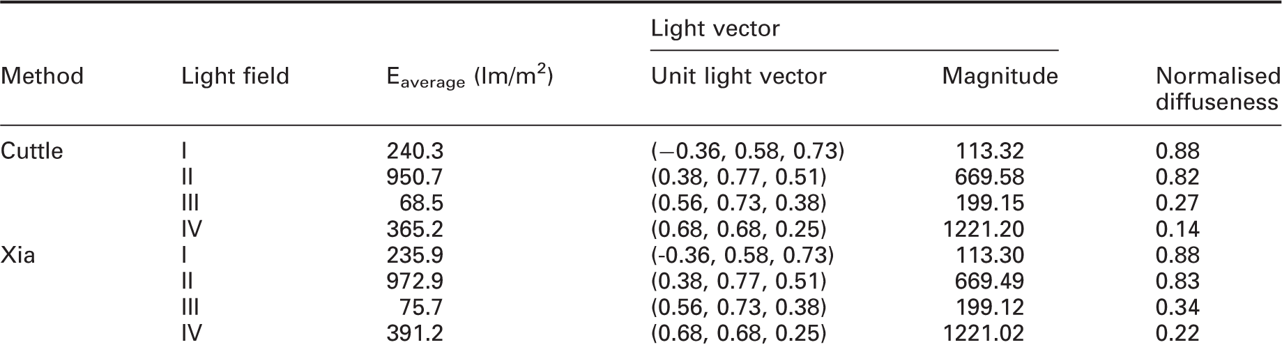
Note: LF I: semi-diffuse light plus white background; LF II: collimated light plus white background; LF III: semi-diffuse light plus black background; LF IV: collimated light plus black background.

6. Visualisation of the global structure of a light field

The measurements in the last two sections concerned local measurements of the light field. However, the light field is also a function of position. If we take into account its dependence on direction and position we get a five-dimensional function. So how can we derive and picture the global structure of a light field? Mury et al.²² managed to visualise the structure of a light field globally over an entire space by using light tubes. The tube’s direction is locally tangential to the light vector (i.e. the direction of net energy transfer) and its width is locally inversely related to the magnitude of that vector (i.e. the larger the net light transport, the smaller the tube). The tubes usually start at light sources, where they are quite narrow, and they end at light absorbing surfaces, where they tend to be quite wide.

The light tubes representation actually shows what lighting architects call the ‘light flow’.^9,27 However, Mury et al.’s light tubes did not carry any information about the diffuseness, which is an essential characteristic of the complete radiant structure of the light field that has a great impact on the appearance of objects inside the room. We suggest using the colour saturation of the light tubes to visualise the diffuseness and the colour brightness to visualise the ‘light density’ of the light field. In this manner, all lower order variables of the global structure of the light distribution in 3D space can be visualised simultaneously and intuitively.

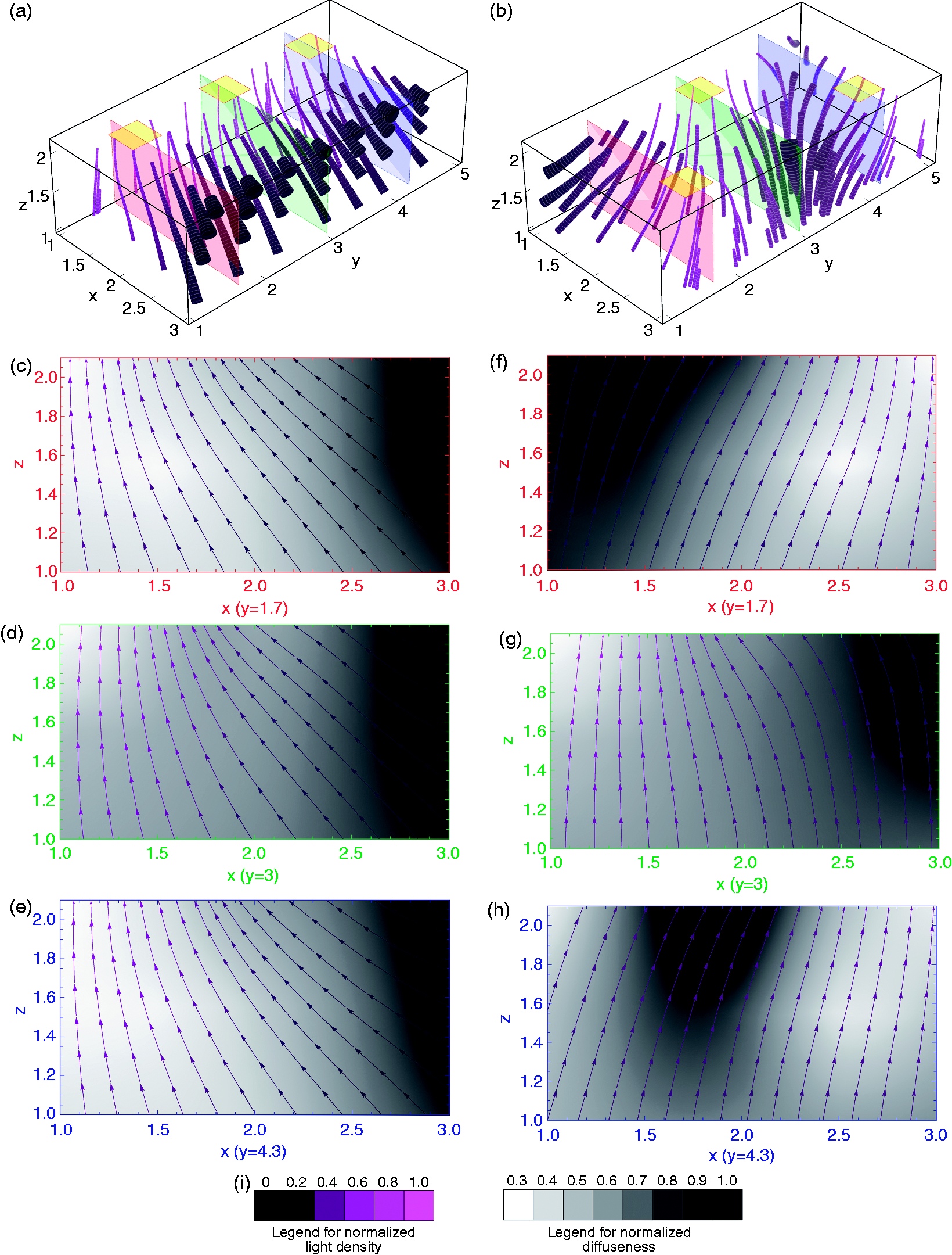
Figure 8(a) and (b) (based on measurements by Mury et al. and available in colour in online version of this paper) shows, as examples, side views of the light tubes in a light lab visualisation using our method. The light lab (i.e. a laboratory space at Philips Research, Eindhoven) was a typical empty office room of 4 by 6 by 3 meters. Figure 8(a) shows the laboratory illuminated by three diffuse area light sources (indicated by the yellow squares) mounted in the ceiling along one of the long walls (hereafter referred to as Light Lab condition A). Figure 8(b) shows the laboratory illuminated by the same sources but now in a triangular configuration (hereinafter referred to as Light Lab condition B). Figure 9(a) and (b) illustrates the arrangements of the light sources in a side view. Figure 8(c) and (d) shows the same ‘light flow’ as Figure 8(a) and (b) but from different perspectives. Figure 8(e) illustrates the colour-coded legend used in Figure 8(a)–(d). The colour saturation from left to right represents the normalised light diffuseness, i.e. the less saturated the colour is, the more diffuse the local light field is. We only show normalised diffuseness values from 0.3 to 1, since they actually range from 0.35 to 0.86 in the measurements. The brightness of the colour indicates the ‘light density’; the brighter the colour, the higher the ‘light density’. The ‘light density’ was normalised to the range from 0 to 1.

Figure 8.

A side view of the ‘light flow’ in a room with three diffuse area light sources mounted in the ceiling (a) along one of the long walls (Light Lab condition A) and (b) in a triangular configuration (Light Lab condition B). The light sources are indicated by yellow squares. A tube’s direction is locally tangential to the light vector, the tube’s width is inversely proportional to the magnitude of the light vector, the saturation of tube’s colour indicates the light diffuseness and the colour brightness is proportional to the light density. Different perspectives of the ‘light flow’ are shown in (c) and (d) (The digital versions of the 3D models can be accessed in the online version which allows interactive manipulation of the view and dynamic change). The legend is shown in (e): the more saturated the colour is, the more directed the local light field, and the brighter the colour is, the higher the light density. The appearance of a white matte sphere for the conditions shown in the legend in (e) is given in (f) (for a light direction: ϑ = 20°, ϕ = 70°) (available in colour in online version).

Figure 9.

The planes that were selected to show the ‘flow lines’ in (a) light lab condition A and in (b) Light Lab condition B. ‘Flow lines’ on planes parallel to the x-z plane when (c) y = 1.7, (d) y = 3.0 and (e) y = 4.3 in Light Lab condition A and (f) y = 1.7, (g) y = 3.0 and (h) y = 4.3 in Light Lab condition B. (i) The legends used: the brighter the colour of the ‘flow lines’, the higher the light density, and the darker the ‘wash’, the more diffuse the local light field (available in colour in online version).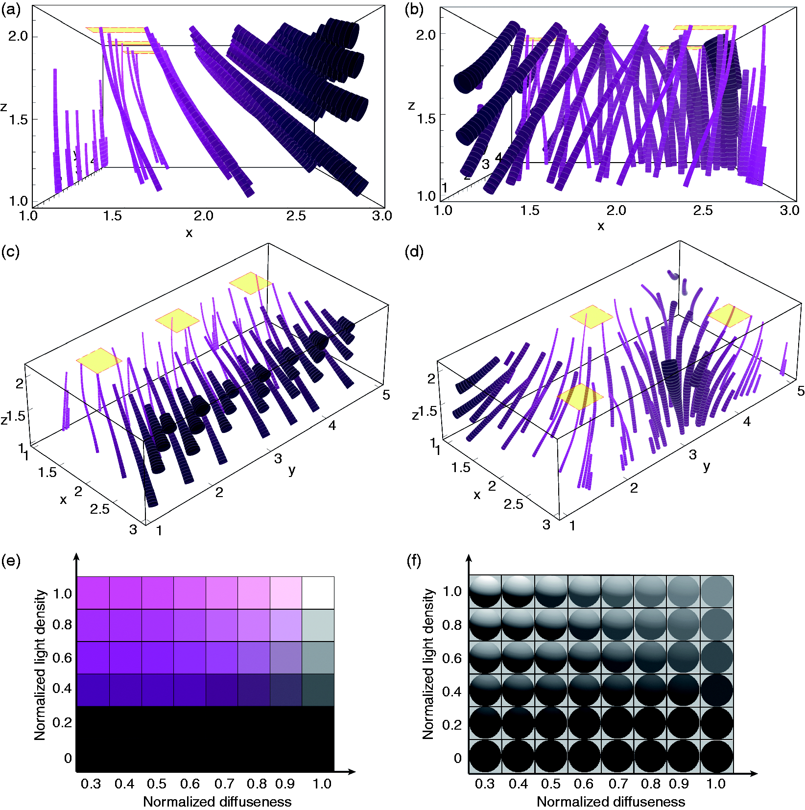

Building on the idea of using ‘light probes’ to visualise light qualities, we also made a legend showing in Figure 8(f) the appearance of a sphere for the conditions shown in the legend of Figure 8(e). For these renderings, we used a combination of collimated and diffuse illumination. The altitude ϑ and azimuth ϕ for the point light source were set at 70° and 20°, respectively, just as an example.

In previous research, a family of flow lines on a plane has been used to characterise the illuminance field in a lighted room.^14,28 The direction of flow lines coincides with the directions of the illuminance vectors and the concentration of the flow lines is directly proportional to the illuminance vector strength. For light fields that are constant along one dimension, drawing the flow lines on one plane is sufficient to visualise the light flow directions. However, this method does not work for most natural light fields since the three-dimensional structure of natural light fields is often not symmetric and in many cases quite complicated. For instance, Figure 9(c)–(h) shows the flow lines on different planes parallel to the x-z plane in Light Lab condition A and light lab condition B. The selected planes are illustrated in Figure 9(a) and (b). Figure 9(i) shows the legends; the brighter the colour of the flow lines, the higher the ‘light density’. The normalised light diffuseness is represented by the gray level of the ‘wash’, i.e., the darker the wash, the more diffuse the local light field is. It is clear that the structure of flow lines is quite similar on the different planes in Light Lab condition A but not in Light Lab condition B. Thus, compared to illustrating flow lines on planes, the light tubes are a more inclusive and intuitive method to visualise the three-dimensional structure of natural light fields. Moreover, the light tubes also show the variations in the strength of the flow.

7. Discussion and conclusions

We introduced a way to simultaneously measure the light density, light vector and diffuseness variations of a light field using a cubic illumination meter. Both with our method and Cuttle’s method using a cubic illumination meter, we can measure the magnitude and direction of the illumination vector quite well but the scalar illumination less accurately. This result agrees with former results, e.g. Ashdown and Eng²⁹ state

One difficulty with cubic illumination meters is that they are sensitive to orientation in the presence of strongly directional lighting, with a maximum possible variance of 33 percent for the scalar illuminance. This is not usually a concern with most office lighting designs, but it can be important for exhibit and theatre lighting.

We applied our method to six light probe images of natural scenes and four real scenes built in our laboratory, and compared the results to those calculated using Cuttle’s method. This comparison showed that both methods could measure the diffuseness accurately and robustly in natural scenes using a cubic illumination meter. We found that care should be taken to maximise the number of lighted meter faces and ensure the illumination diversity on six faces.

Finally, we demonstrated a way to simultaneously and intuitively visualise the global structure of a light field up to its first-order properties or spatial variations of the light density, vector and diffuseness using light tubes. Furthermore, via a legend we visualised the light effects on the appearance of a spherical ‘light probe’. It might seem a good idea to directly render such probes within a space to visualise the light field. However, we think the light tubes approach works better, because judgments of light direction and diffuseness from the appearance of a white sphere are confounded due to basic image ambiguities.^30,31 For example, observers confused more frontal illumination with higher levels of diffuseness.⁸ This was also found in a practical test.¹⁰

Besides using a cubic illumination meter, other methods can be used to measure the light scalar and vector. One example is a half table-tennis ball photosensor mounted on a two-axis mechanical stage proposed by Fuller et al.³² (or its modern version using a light meter app on a smart phone plus a hemispherical diffuse cap). Dale et al.²⁸ proposed another simple way to infer the light vector using a grease-spot device. Both methods are intuitive in providing information about the light vector. In Fuller et al.’s setup the light vector lies along the direction where the photosensor reaches the maximum value. In Dale et al.’s setup the light vector lies in the plane of the grease-spot device when the difference between grease-spot and its surround paper vanishes because both sides have the same illumination. In Fuller et al.’s setup, taking another reading by rotating the tennis ball photosensor by 180° to the opposite direction of the light vector, the light scalar can be calculated as half of the sum of both readings. In Dale et al.’s setup, however, there is no direct way to get the light scalar. Nevertheless, rotating the mechanical stage and the grease-spot both need a lot of effort. Apart from the two experimental setups mentioned above, it is known that the average of the illuminance on the four sides of a regular tetrahedron is close to the scalar illuminance³³ However, the light vector cannot be measured robustly by the illuminance on the tetrahedron faces (we have also verified this point using our SH approach).

The novel diffuseness metric D_X_ia is conceptually equivalent with D_C_uttle but with different methods to recover their values. Nevertheless, each of these two methods has its advantages and disadvantages. Cuttle’s method requires only simple calculations that can be done with a pen and a piece of paper. Thus, Cuttle’s method is most suitable for a quick, local estimation of the diffuseness level in a natural scene. In contrast, our SH representation based method needs computation software on a computer in order to fit the SH representation to the data. The SH representation based D_X_i_a, together with the light flow and light density forms a global, integrated description of the lower order properties of the light field distribution in a three-dimensional space. This method fits all parameters being described within one integral description/decomposition, in which it is clear how the parameters relate and which role they play in the resulting light field. With the development of lighting modelling and rendering software, the SH method will have more and more advantages in fast, real-time rendering. Furthermore, in lighting design, software tends to be used more and more as an assisting tool. HDR environment maps were already used widely in computer graphics. Currently, lighting design software can also export such maps easily. We suggest to provide the light density, light vector and D_X_i_a, together with the HDR environmental maps in order to give lighting and graphics designers a reference of the ambient, direction and diffuseness levels. Moreover, next to this local description for a single HDR map our method provides insights into the global structure of the light field in three-dimensional spaces. Light distributions in natural spaces show spatial variations of the ambient, vector and diffuseness, which can be captured using simple cubic illumination meter measurements and visualisations of interpolated data, e.g. the light flow representation using light tubes, as we demonstrated.

Mury et al.^22,34,35 described the light field in terms of the lower order SH approximation and successfully measured its components in natural scenes. The main contribution of this study is that we extended the work of Mury et al. by adding description, measurement and visualisation methods for the diffuseness characteristic or, in other words, we re-framed the diffuseness metric of Cuttle into an integral description of the light field. This approach makes it possible to progress towards the third stage of the lighting profession as Cuttle described the innovative step lighting science should take towards dealing with light instead of lamps.⁷

Footnotes

Funding

The author Ling Xia is supported by the Chinese Scholarship Council (CSC program).

Appendix: Construction of a cubic illumination meter

References

Kelly

. Lighting as an integral part of architecture. College Art Journal 1952; 12: 24–30.

Kelly

Neumann

Addington

. The Structure of Light: Richard Kelly and the Illumination of Modern Architecture, New Haven, CT: Yale University Press, 2010.

Cuttle

. A new direction for general lighting practice. Lighting Research and Technology 2013; 45: 22–39.

Boyce P. Lighting quality for all: Proceedings of SLL and CIBSE Ireland International Lighting Conference, Dublin, Ireland, 12 April: 2013.

Kelly

Duff

. Lighting design in Europe: Aligning the demands for lower energy usage with better quality. Journal of Civil Engineering and Architecture 2015; 9: 283–290.

Cuttle C. Perceived adequacy of illumination: A new basis for lighting practice: Proceedings of the 3rd Professional Lighting Design Convention, Professional Lighting Designers Association, Madrid, Spain, Oct 19–22: 2011: 27–31.

Cuttle

. Towards the third stage of the lighting profession. Lighting Research and Technology 2010; 42: 73–93.

Pont

Koenderink

. Matching illumination of solid objects. Perception and Psychophysics 2007; 69: 459–468.

Cuttle

. Lighting patterns and the flow of light. Lighting Research and Technology 1971; 3: 171–189.

10.

Madsen M, Donn M. Experiments with a digital “light-flow-meter” in daylight art museum buildings: 5th International Radiance Scientific Workshop, Leicester UK, September 13–14: 2006.

11.

Koenderink

Pont

van Doorn

Kappers

AML

Todd

. The visual light field. Perception 2007; 36: 1595–1610.

12.

Koenderink

van Doorn

Kappers

AML

Pont

Todd

. The perception of light fields in empty space. Journal of Vision 2005; 5: 558–558.

13.

Te Pas SF, Pont SC. A comparison of material and illumination discrimination performance for real rough, real smooth and computer generated smooth spheres: Proceedings of the 2nd Symposium on Applied Perception in Graphics and Visualization, Spain: ACM, August 26–28: 2005: 75–81.

14.

Gershun

. The light field (translated by Moon, PH and Timoshenko, G). Journal of Mathematics and Physics 1939; 18: 51–151.

15.

Mury

. The light field in natural scenes, Delft: Faculty of Industrial Design Engineering, Delft University of Technology, 2009.

16.

Frandsen S. The scale of light – A new concept and its application:Proceedings of the 2nd European Conference on Architecture, Paris, December 4–9: 1989: 4–8.

17.

Hewitt

Bridgers

Simons

. Lighting and the environment: Some studies in appraisal and design. Lighting Research and Technology 1965; 30: 91–116.

18.

Cuttle C, Valentine W, Lynes J, Burt W. Beyond the working plane. Proceedings of the CIE, Washington, DC, June 19–28: 1967, P-67-12.

19.

Morgenstern

Geisler

Murray

. Human vision is attuned to the diffuseness of natural light. Journal of Vision 2014; 14: 1–18.

20.

Cuttle

. Cubic illumination. Lighting Research and Technology 1997; 29: 1–14.

21.

Cuttle

. Research note: A practical approach to cubic illuminance measurement. Lighting Research and Technology 2014; 46: 31–34.

22.

Mury

Pont

Koenderink

. Representing the light field in finite three-dimensional spaces from sparse discrete samples. Applied Optics 2009; 48: 450–457.

23.

Ramamoorthi

Hanrahan

. On the relationship between radiance and irradiance: Determining the illumination from images of a convex Lambertian object. Journal of the Optical Society of America A 2001; 18: 2448–2459.

24.

Debevec P. Rendering synthetic objects into real scenes: Bridging traditional and image-based graphics with global illumination and high dynamic range photography: Proceedings of ACM SIGGRAPH 2008 classes, Los Angeles, CA: ACM, August 11–15: 2008: Vol. 32:1–10.

25.

Debevec P. High-resolution light probe image gallery. Retrieved 12 January 2016, from: http://gl.ict.usc.edu/Data/HighResProbes/.

26.

Xia

Pont

Heynderickx

. The visual light field in real scenes. i-Perception 2014; 5: 613–629.

27.

Lynes

Burt

Jackson

Cuttle

. The flow of light into buildings. Transactions of the Illuminating Engineering Society (London) 1966; 31: 65–91.

28.

Dale

Broadbridge

Crowther

. Measuring the direction of the flow of light. Lighting Research and Technology 1972; 4: 43–44.

29.

Ashdown I, Eng P. The virtual photometer: Modeling the flow of light: Proceedings of IESNA 1998 Annual Conference Technical Papers, San Antonio, TX, August 10–12: 1998.

30.

Belhumeur

Kriegman

Yuille

. The bas-relief ambiguity. International Journal of Computer Vision 1999; 35: 33–44.

31.

Koenderink

Pont

. Irradiation direction from texture. Journal of the Optical Society of America A 2003; 20: 1875–1882.

32.

Fuller

Upton

Whalen

. The photometry of the flow of light. Lighting Research and Technology 1971; 3: 282–284.

33.

Singleton

. The Body at Work: Biological Ergonomics, Cambridge: Cambridge University Press, 1982.

34.

Mury

Pont

Koenderink

. Light field constancy within natural scenes. Applied Optics 2007; 46: 7308–7316.

35.

Mury

Pont

Koenderink

. The structure of light fields in natural scenes. Applied Optics 2009; 48: 5386–5395.