The effect of assuming static or dynamic gaze behaviour on the estimated background luminance of drivers

Abstract

Application of the Commission Internationale de l’Eclairage system for mesopic photometry requires that an estimate is made of the observers’ state of luminance adaptation. This paper addresses an assumption made when estimating background luminance, a component of adaptation luminance. Specifically, using spatial sampling of the visual field we compare background luminances determined from assumptions of static or dynamic visual gaze, the former being a simplification, the latter being a better representation based on eye movements when driving. The comparison was undertaken with luminance images of urban scenes at night on three roads, two real and one simulated. It was found that background luminances were significantly higher when estimated using the dynamic assumption. It was also found that scene luminances at the point of foveal fixations tend to be higher than those luminances influencing peripheral regions of the retina. Compared with the background luminance estimated for a dynamic peripheral field, a horizon-centred 10° circle led to a slightly higher estimate and the road surface luminance to a slightly lower estimate of background luminance.

1. Introduction

The Commission Internationale de l’Eclairage (CIE) proposed system of mesopic photometry¹ is a system for characterising the spectral efficiency of visual performance at low levels of light according to relative contributions of cone (photopic) and rod (scotopic) photoreceptors. This is determined using the S/P ratio of the ambient illumination and the luminance to which the eye is adapted. CIE technical committee JTC-1 has the objective of seeking a method for estimating the state of visual adaptation of road users in order to guide application of the mesopic system; this paper focuses on drivers of motorised vehicles.

Estimation of the state of adaptation of a driver is not a new task in itself, with guidance already available for tunnel lighting,² for assessing the influence of glare via the threshold increment (TI)^3–5 and for calculating the visibility level of a small target.⁶ In these, adaptation luminance (L_a) is estimated as the sum of the background luminance (L_b) around a task and the veiling luminance within the scene caused by surrounding sources of high luminance (L_v): L_a = L_b + L_v.^7,8 This approach takes into account the scattered light due to glare within the visual field.⁹ The aim of estimating adaptation for these purposes is, however, to consider the visibility of a target, foveally fixated and static against its background, typically the road surface. In contrast, determination of mesopic luminance requires an estimate of the adaptation state of the peripheral regions of the retina rather than the fovea.

Adaptation is the process of adjusting to the quantity and quality of light: if the eye is exposed for a sufficient time to a uniform condition every part of retina reaches a steady state and the eye can be said to be adapted to that level of light.¹⁰ Estimating the state of adaptation within a homogeneous field is relatively straightforward: in typical laboratory trials this is the luminance of the uniform background surrounding a fixation point.^11–13 Estimating the state of adaptation of a driver in the natural setting is not straightforward, however, because the visual scene is likely complex and inhomogeneous. This arises because a single scene is likely to present a range of luminances rather than a uniform luminance, and because the dynamic nature of eye movements and travel along a road mean a number of fields are seen in succession. Different parts of the retina will therefore be differently adapted depending on where, and for how long, gaze is directed.^14,15

For foveal adaptation, one way to estimate the L_a would be to look at the pattern of fixation points and the time spent at each:¹⁵ Uchida et al. proposed a method for doing this which took into account eye movements among other parameters.¹⁶ A simpler but possibly less accurate approach would be to use the average luminance of a region of the observed scene in which the majority of fixations were expected to occur. One suggestion is to use a circular field with an angular diameter of 10°–20°,⁸ this being approximately confirmed by eye tracking data.¹⁷

Eye movements comprise two parts, saccades and fixations. Fixations are periods of time, where the gaze rests at a particular position, e.g. when assessing a traffic scene regarding action that needs to be undertaken (we ignore here the miniature movements – tremor, drift and micro-saccade – that occur during a fixation¹⁸). Saccades are the rapid movements of the eye between successive fixations. Eye movements are used in a feed-forward role to the motor system, to locate the information needed for the execution of an act.¹⁹ Note, however, that fixation on an object or area does not imply for certain where the observers attention is focused – gaze location does not uniquely specify the information being extracted.²⁰ However, when exposing the retina, or, more precisely, particular parts of it to a light scene, the mechanisms of adaptation are triggered regardless of attention. Of course the longer a gaze rests at a particular part of the road lured by attention, the more likely will the transient re-adaptation process be to converge, i.e. to complete the process as defined by Moon and Spencer.¹⁰

The gaze direction of a driver is dynamic, constantly moving to different regions of the visual field, in part determined by experience and distractions.^17,21–23 As a result, different parts of the visual field stimulate different parts of the retina, and this puts the retina into a state of continuous transient adaptation.²⁴ Transient adaptation is the state of changing adaptation when the visual system is not completely adapted to the prevailing illumination, e.g. when gaze is moving around in a road scene or when looking from the outside to the inside of the vehicle.¹⁵ If these changes of exposure to different luminances are within ±2 log units, transition happens very fast.⁷ Other findings however indicate that the duration required for the transition depends on whether the change is from low to high or from high to low luminances.²⁵ When driving along a road, the visual field constantly changes, which, therefore, puts the retina into a continuous state of transient adaptation. Although certain areas change very little, e.g. the road surface, other areas such as shop facades, advertisements etc. present a larger change in luminance.

In one recent study the combined eye-movement and luminance measurements along a road were analysed, with estimates of the visual adaptation calculated as the mean luminances of circular fields of various sizes (1°–20° in diameter) centred around the fixations of drivers.²¹ A second study examined mean luminances within various elliptical and circular fields of size 1°–90°, centred 1° below the horizon at the centre of the lane and compared these to the mean luminance on the road surface.²⁶ Other studies suggest that only the local luminance (i.e. the luminance at and around a task point) influences visual performance, which is an estimate for adaptation.^10,27–30 That assumption would make field sizes larger than 2° around an assumed static task point irrelevant.

In summary, while methods for estimating adaption luminance assume a static, uniform and fixed field of view, driving in real situations involves dynamic eye movements across a non-uniform visual field. This paper investigates L_b, one of the two components of L_a and suggested by Maksimainen et al.²⁶ to be the more significant component for the calculation of mesopic luminances. Specifically, this paper explores the change in L_b found if the visual field is assumed to be dynamic rather than static. This is examined for both foveal and peripheral visual fields.

2.Method

2.1. Luminance data

The L_b component of adaptation was estimated using different approaches using luminance data from three roads and eye tracking data recorded in a natural setting.

Luminance images were gathered from three types of road, these being two real urban traffic scenes (a main road and a residential street as investigated using eye tracking¹⁷) and one simulated traffic scene (Table 1). The simulated scene is included because it is very likely that application of the mesopic luminances will be within the design process, which is typically done with simulation programs. The simulation was undertaken with a framework based on the software Radiance.³¹

Table 1

Description of the three roads for which the luminance images were gathered.

Type of road¹	Road characteristics	Luminaire positioning/ spacing	Lighting class²	Road surface characteristics
Main road (OS)	Four lanes, separated carriageways, parked vehicles on right side	Opposite, 32 m	M2	unknown
Residential street (EA)	Two lanes, parked vehicles on both sides	Irregular Staggered, 55 m³	M6	unknown
Simulated road (TS)	Two lanes	One-sided, 39 m	M5	R3

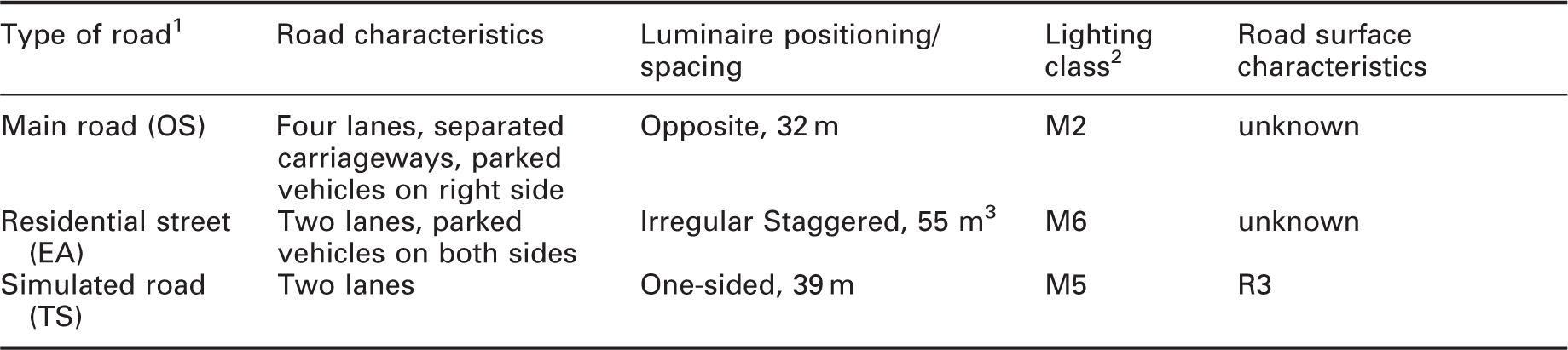
¹OS, EA and TS are abbreviations of the road names: OS: Otto-Suhr-Allee; EA: Eschenallee; TS: Treskowstraße.

²Lighting class as estimated from CIE115:2010⁴, annex E.

³The installation did not follow a regular left-right-left-right staggered pattern. The luminance images were recorded at 10 uniform intervals over a 55 m section which comprised lamp posts on the right, left, left and right.

Scene luminances were established at ten regular intervals in each road. The measurement in the two urban traffic scenes was undertaken with a TechnoTeam LMK Color 4 with an 8 mm lens (approximately 63° × 45° field of view) from within a vehicle from behind the driver’s seat (see Figures 1 and 2). The simulation resulted in images with the same size and field of view.

Figure 1

Photograph of the interior of the test vehicle to illustrate the location of the fixed image luminance measurement device (mounted behind the driver’s seat), which was used to gather a static luminance image series between two luminaires.

Figure 2

Images taken from the driver’s view point at the ten locations in each of the three roads: residential street (top), main road (middle), simulated road (bottom).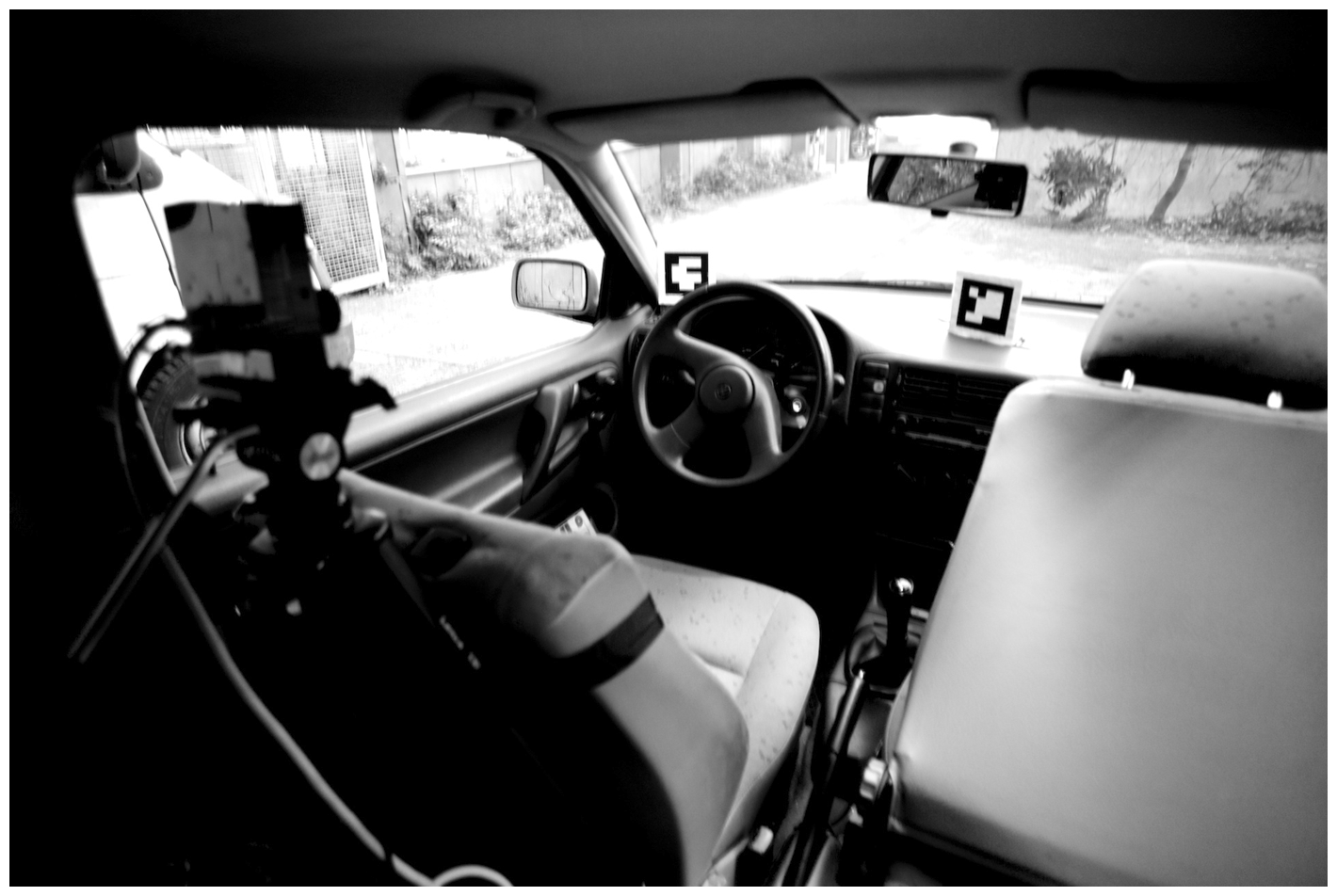

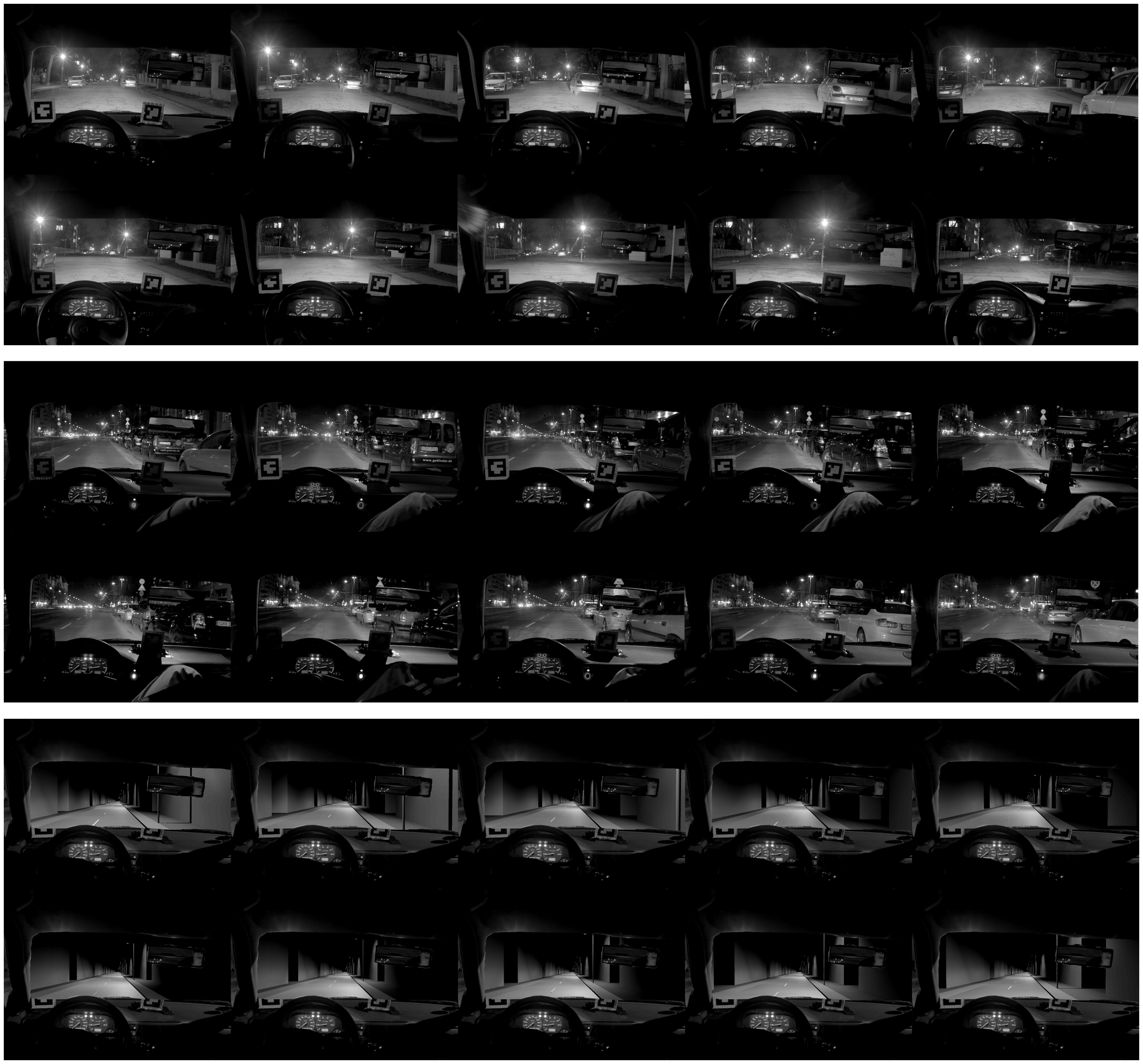
The images captured on the main road (OS) contain approaching traffic and a traffic signal close to an intersection. The images taken on the residential street (EA) are free of approaching traffic, as are the images from the simulated road. As the images were captured from within a vehicle from the driver’s perspective they included the interior of the vehicle. To make the simulated images comparable to the measured images of the real scenes the pixels containing the luminance values of the interior of the vehicle captured on the residential street were copied to the corresponding positions in the simulated luminance image. The headlamps of the vehicle were switched on during field measurement; this was not the case in the simulated images in accordance with current lighting design standards which do not account for headlamps of cars.^4,5

2.2. Estimation of foveal L_b based on eye movement

One proposal for estimating the state of adaptation is to consider the pattern of eye movements and the duration spent at each location.^15,16 The L_b can thus be estimated using the weighted mean luminance of a luminance image L(x,y) of a given road scene, using an eye movement data map EM(x,y) to provide the weighting (equation (1)).

{\bar{L}}_{b, weighted} = \frac{1}{\sum_{x = 1, y = 1}^{x = width, y = height} EM (x, y)} \times \sum_{x = 1, y = 1}^{x = width, y = height} EM (x, y) L (x, y)

(1)

Equation (1) summates for each pixel (at coordinates x,y) the luminance of that pixel (L (x,y)) as weighted by the frequency for which the cumulated eye tracking data¹⁷ suggest that pixel is fixated (EM (x,y)). To estimate the weighted mean luminance of the scene, this summation is divided by the total frequency of these observations.

We use here the eye movement data of car drivers in urban environments at night reported in a previous study.¹⁷ These were eye movements of 23 people when driving along two straight roads, a main road and a residential street (Table 1). For the current purpose we are interested in typical gaze behaviour, and for simplicity are considering straight sections of road. It has been shown that different types of road may yield different patterns of gaze behaviour, according to the location of expected hazards, but that different sections of the same type of road tend to yield similar distributions of gaze.¹⁷ These roads were a main road (1.46 km) and a residential street (1.14 km). To estimate the proportion of travel time for which the fovea was directed to a particular direction within the scene, the fixations occurring along the whole length of each road were (separately) summated. In other words, the cumulative fixation point data for the whole road were used in the analysis of each of the ten sections of that road.

2.3. Estimation of peripheral L_b

Different parts of the retina are exposed to different parts of the scene and thus, for a scene of non-uniform luminance distribution, different parts of the retina will be subject to different states of adaptation. As the application of mesopic luminances is for visual performance in peripheral vision, then what is of interest here is the adaptation state of the peripheral retina. The method described above, i.e. the weighted mean of eye movement data and a luminance image represents a means for estimating the state of foveal adaptation; the estimation of the state of peripheral adaptation needs another approach.

To analyse this issue four factors play a role: the spatial extent of the retina, the spatial distribution of the scene, the movement of the eye and the movement along the road.

2.3.1. Spatial sampling of the visual field

Figure 3 shows the sampling fields used to investigate changes in scene luminances. This is a field of diameter 20° centred on the fovea. Within this, luminances are calculated for each of 69 evenly distributed sub-areas, each being a 2° circle, with the central sub-area being superimposed on the fovea. The 20° size was chosen because the experiments contributing to CIE 191¹ used a 10° off-axis target which falls at the perimeter of this schematic.^11–13 We first assumed the whole of this field to be relevant, but also investigated the effect of ignoring the upper part of the field assumed to be less critical for drivers.

Figure 3

Schematic of the spatial sampling of the visual field, where the central 2° circle represents luminances to which the fovea is exposed, and extending to a diameter of 20°. The 69 sub-areas are each 2° circles, these arbitrarily chosen for analysis of luminance variations across the visual field.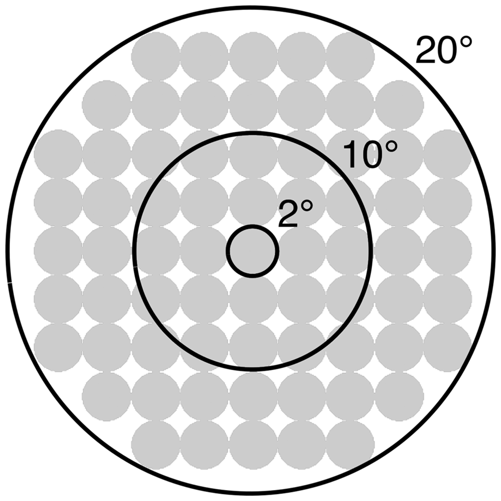

The purpose of adopting these sampling fields is to illustrate the range of luminances to which different parts of the retina might be exposed to in a given situation, as indicated by Wördenweber et al.¹⁴ (page 271) and based on the method of spatial sampling.³² We recognise that light will also fall into the spaces between the circular sub-regions, but the additional precision produced by including these data is not required for the current analysis. Note that these circular areas are not intended to represent receptive fields, i.e. the collated activity of a number of photoreceptors, which increase in size with increasing eccentricity and decreasing luminance,¹⁵ nor does this simplified model intend to cope with the curvature or optics of the eye.

2.3.2. Static assumption

Consider the sampling fields overlaid on a road scene. It is common in road lighting to assume a static fixation point, such as when assessing glare³ or visibility.⁶ Figure 4 reveals the range of luminances the retina can be assumed to be exposed to with static fixation on an example road scene (here the simulated road TS). In this case it is assumed that the field of view was centred at the horizon of the lane, as identified in previous research.¹⁷ The luminances in Figure 4 were determined from the simulated road scene, the purpose being to illustrate the change in these mean luminances with the change from static to dynamic assumptions. While we expect that the range of luminances encountered in real scenes would vary and may be higher or lower than these²⁵ we do not expect that the change between static and dynamic assessments would change. To estimate L_b for the foveal static field we used the average luminance of pixels in the central 2° field of the sampling pattern.

Figure 4

Assuming a static fixation at the centre of lane at the horizon this visualisation shows the various mean luminances to which the retina is exposed on the simulated road TS. These numbers are the exponent of the mean luminance within each of the 2° circular patches distributed across the visual field. The white circles indicate visual field sizes of 2°, 10° and 20°. Note that the maximum values within the patches, especially the ones with the very bright pixels of the fixed road lighting can be as high as 35 kcd/m².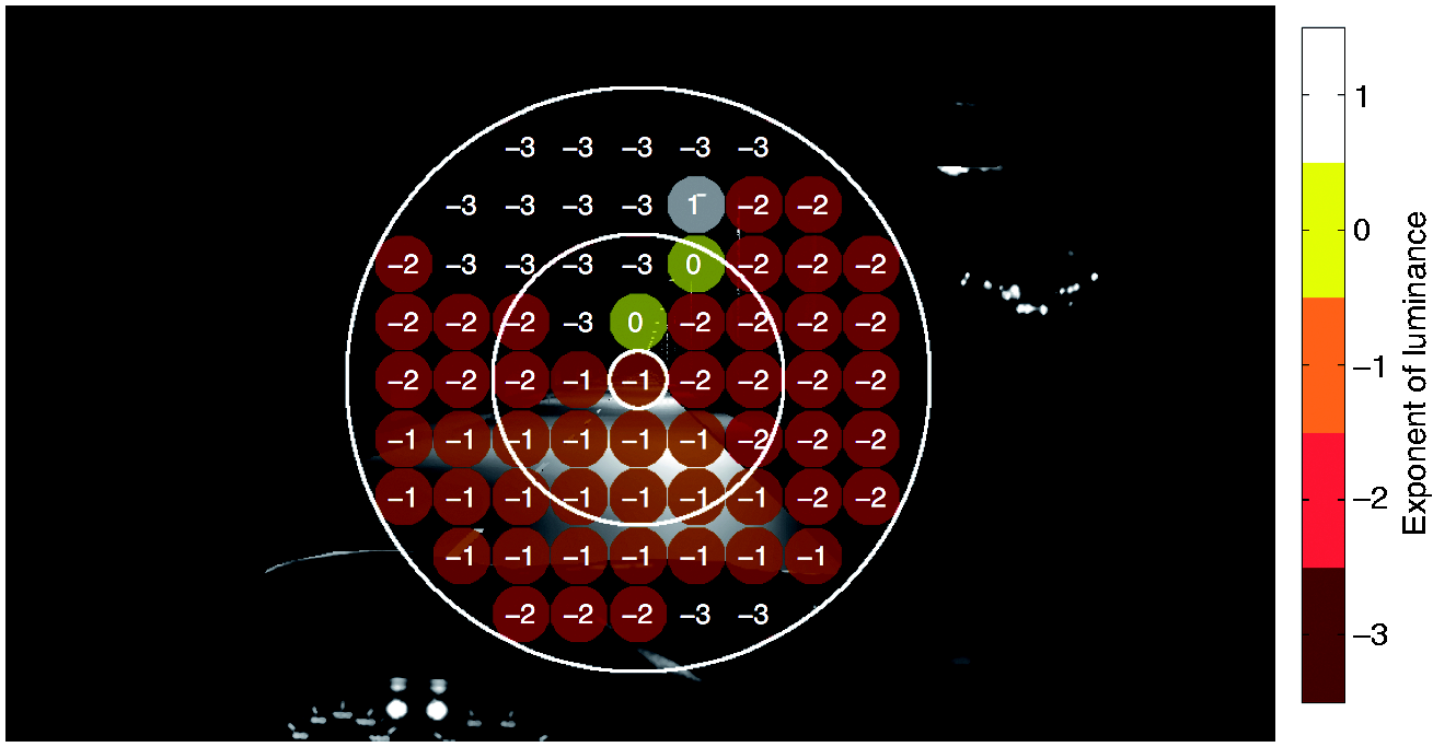

The peripheral areas of the retina exposed to the road surface are influenced by luminances with an exponent of −1, i.e. in the range 0.99–0.10 cd/m², the left and right peripheral areas are influenced by the surrounding buildings (simulated five-storey housing with a grey concrete surface) with luminances having an exponent of −2, i.e. in the range 0.099 − 0.01 cd/m, and the areas exposed to the sky are influenced by the rather dark luminances with an exponent of −3, i.e. in the range 0.0099 − 0.001 cd/m². Some areas are influenced directly by the light sources, which were as bright as 35 kcd/m² in this example of the simulated street (although in Figure 4 the exponent is lower due to reporting the mean luminance within a 2° circular area). In real road scenes the surrounds tend to be brighter (with a luminance of about 10⁻²cd/m² in the residential street EA and about 10⁻¹cd/m² in the main road OS) and there may be more sources of glare (such as the headlamps of approaching vehicles or the tail-lights or brake-lights of vehicles ahead) which would be additional contributors to the scene as well as the headlamps of one’s own vehicle.

2.3.3. Dynamic assumption

Next, consider how eye movement behaviour effects the estimate of luminance projected to a specific part of the retina. The eye does not look straight ahead but tends to scan the visual field, with a pattern that is different for different observers. To represent this, we used the eye movement data of 23 drivers, as captured using mobile eye tracking in two roads.¹⁷ These data are a step towards representing where most of the people tend to look at most of the time, rather than the gaze behaviour of a single observer or an assumed static fixation.

Figure 5 (left) shows a sample scene upon which are mapped the accumulated locations of visual fixations toward that scene as determined using eye tracking.¹⁷ The sampling fields were overlaid upon each of these fixations, aligning the region assumed to influence the fovea to the centre of each fixation point (Figure 6). For each fixation the scene luminance was established for each sub-area of the sampling fields (scene luminance here being the mean luminance of pixels contained in each sub-area). The weighted mean luminance of each sub-area of the sampling fields was then determined across all fixations, thus representing what each sub-area of the retina was exposed to, based on the relative proportion of time the fovea, and therefore the whole retina, was exposed to a particular direction. For each of the roads that process was undertaken for each of the ten locations at regular intervals between two lamp posts for which luminances were determined (Section 2.1). Or, in other words, the method for calculating a weighted luminance as described in equation (1) was undertaken for each of the 69 sub-regions of the spatial sampling of the visual field. To estimate L_b for the foveal dynamic field we used the weighted luminance of pixels in the central 2° field of the sampling pattern.

Figure 5

Example of the process for simulating the probable luminance to which a particular sub-area of the sampling fields was exposed to based on eye movement. A weighted mean luminance was calculated for each of the 69 sub-areas (+ represents a fixation within the scene/the fovea within the sampling fields). Note that the graphic of the sampling fields is just a mock-up and does not consist of 69 sub-areas. Figure 6 depicts the procedure more precisely.

Figure 6

The calculation of the weighted mean luminance for each of the 69 sub-areas was undertaken as follows: for each fixation (+) of the eye movement data the mean luminance of each 2° sub-area of the sampling fields was calculated, summed up and divided by the number of fixations. Note that the change of grey value in the lower part represents the weighted mean luminance of each of the 69 sub-areas.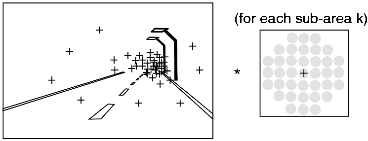

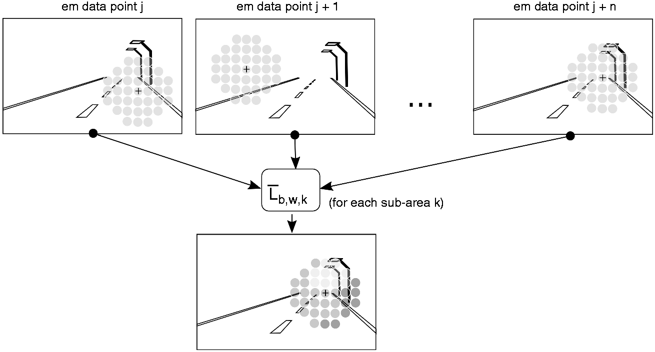
Figure 7 reveals the range of weighted mean luminances the various parts of the sampling fields are exposed to on the simulated street (TS). Comparing Figure 7 with Figure 4 it is evident, that due to distribution of eye movements, a larger part of the sampling fields are exposed to the very bright light sources. The areas of the retina exposed to very low luminances in the assumed static fixation are now shown to be influenced by higher luminances. The lower areas of the sampling fields are mostly influenced by the road surface and remain within the same range of the exponent of the luminance.

Figure 7

Distribution of weighted mean luminances for the simulated road TS. The numbers are the exponent of the weighted mean luminance within each of the 2° circular patches distributed across the sampling fields, estimated assuming that the gaze is dynamic and each particular sub-area of the assessment pattern has a certain probability to be exposed to a particular part of the scene. Note that compared to Figure 4 each weighted mean luminance within the sampling fields is based on eye movement data and contrary to Figure 4 this visualisation does not represent the position of the sampling fields within the scene (which was centred to the horizon at the centre of lane for Figure 4). The white circles indicate the diameter of visual field sizes of 2°, 10° and 20° within the sampling fields.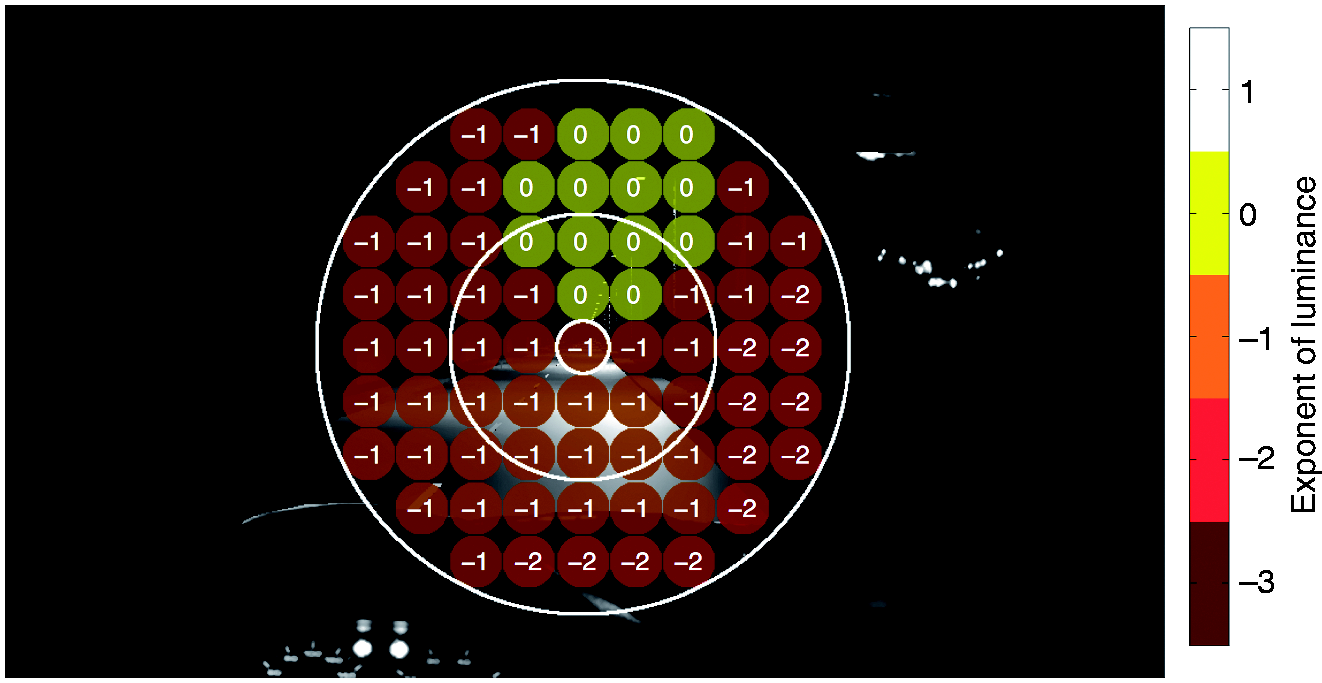

3. Results

Two methods were used for estimating L_b within the field of view: a static approach (the fixed field of view) and a dynamic approach which considered the dynamic eye movements of a driver. The dynamic approach is intended to represent typical gaze behaviour, thus to estimate the relative proportion of time for which regions of the retina are exposed to a particular direction within urban street scenes after dark.

Figures 8 to 10 illustrate mean luminances representing the static assumption (on the left) and weighted mean luminances representing the dynamic assumption (on the right) for two of the ten locations along each road, one being a more homogeneous section (top rows of each Figure) and the other a more heterogeneous section (bottom rows).

Figure 8

Mean luminances within each of the 69 sub-regions of the simplified visual field for two locations of residential street EA. The top row and bottom row show examples of two locations. The luminances are determined according to the static (left-hand column) and dynamic (right-hand column) assumptions of gaze behaviour. Note that luminances shown as 0.0 indicate <0.1 rather than zero.

Figure 9

Mean luminances within each of the 69 sub-regions of the simplified visual field for two locations of main road OS. The top row and bottom row show examples of two locations. The luminances are determined according to the static (left-hand column) and dynamic (right-hand column) assumptions of gaze behaviour.

Figure 10

Mean luminances within each of the 69 sub-regions of the simplified visual field for two locations of simulated street TS. The top row and bottom row show examples of two locations. The luminances are determined according to the static (left-hand column) and dynamic (right-hand column) assumptions of gaze behaviour. Note that luminances shown as 0.0 indicate <0.1 rather than zero.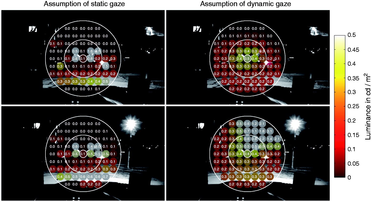

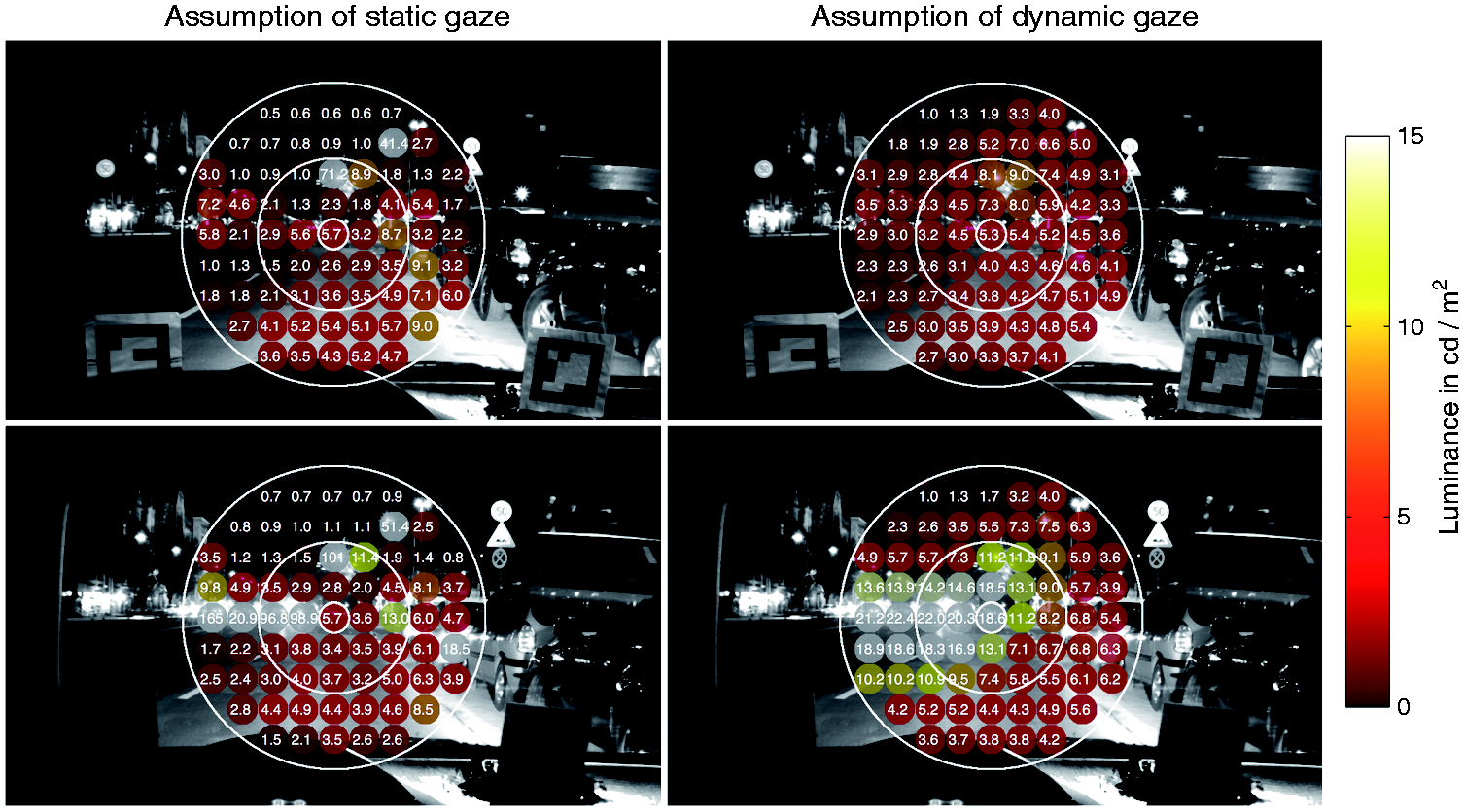
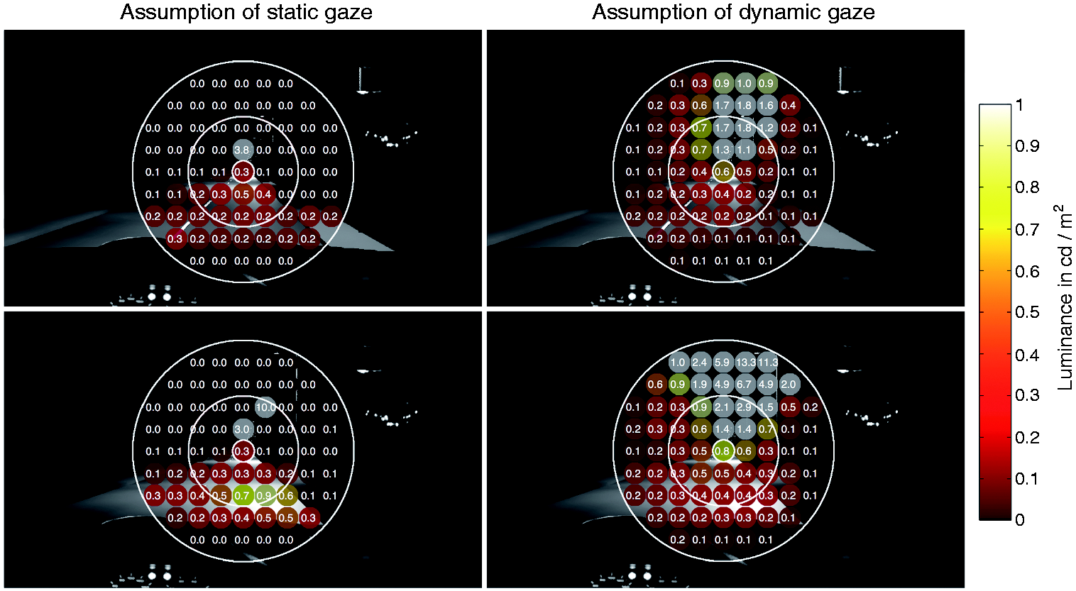
First, note that when the visual scene includes sources of high luminance (such as the headlamps of approaching vehicles or the fixed road lighting installation) the dynamic approach shows that these influence a wider part of the field of view than does the static approach. This can be seen by comparing the left and right hand images of the bottom rows of Figures 8 to 10.

Statistical analysis was carried out with three independent variables: equivalent retinal location within the sampling fields, road type and static versus dynamic assumption. The dependent variable was mean luminance. Factor levels for retinal location were foveal and peripheral, where foveal consisted of the results of the central 2° circle and peripheral the 68 sub-regions surrounding the fovea. Road type consisted of three levels: residential street EA, main road OS and simulated street TS. The factor assumption comprised levels static and dynamic. Ten images were captured between two lamp posts along each road, which resulted in ten samples for each of the foveal retinal location factor combinations and 680 samples for each of the peripheral retinal location factor combinations. It was not intended to compare road types with each other as expected luminance differences were present by definition of the road lighting classes of CIE 115;⁴ the roads were chosen to reassemble different classes.

Mean luminances from nine of the twelve factor combinations were not suggested to be normally distributed according to the Shapiro–Wilk test (p < 0.05). Foveal dynamic EA and TS and foveal static TS were normally distributed (p ≥ 0.24). Hence the statistical analyses were carried out using non-parametric tests of difference. The Wilcoxon paired signed rank test was used for comparing factor assumption (static vs. dynamic). The Wilcoxon rank sum test was used for comparing factor retinal location (foveal vs. peripheral), this alternative test being used because the compared items were of unequal sample sizes (N = 10 within foveal observations and N = 680 within peripheral observations). Effect sizes were calculated as $r = Z / \sqrt{N_{1} + N_{2}}$ ^33,34 and interpreted according to Cohen,³⁵ i.e. absolute value < 0.1 = negligible effect size, ≥ 0.1–0.3 = small effect size, >0.3–0.5 = medium effect size and ≥0.5 = large effect size.

3.1. Static versus dynamic

Figure 11 compares mean luminances estimated following the static and dynamic assumptions, for the three roads, for the foveal and peripheral fields. The medians of the mean luminances estimated with the static assumption are lower than those estimated using the dynamic assumption in all six comparisons. The Wilcoxon paired signed rank test suggests the difference to be significant in five cases (p < 0.05, large effect sizes for foveal comparisons, small effect sizes for peripheral comparisons except TS, which had a medium effect size) but does not suggest a difference for the foveal field on main road OS (p = 0.13, small effect size).

Figure 11

Boxplot comparing the static assumption to the dynamic assumption based on the calculated mean luminances for i = 10 images for the foveal retinal location and for i = 10 images with k = 68 sub-areas each for the peripheral retinal locations (significant differences with p < 0.05 are indicated with *, n.s. otherwise). Note that the data of simulated street TS do not contain headlamps of one’s own vehicle.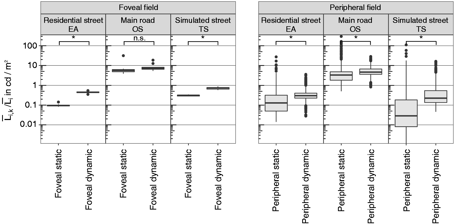

3.2. Foveal versus peripheral

Figure 12 shows the same data as Figure 11 but redrawn to facilitate direct comparison of location in the visual field, i.e. foveal versus peripheral. In five cases, the median of the mean luminances of the peripheral field locations is lower than that of the foveal field (p < 0.05, Wilcoxon rank sum test, small effect sizes). For residential street EA and the static assumption, the difference between foveal and peripheral fields is not suggested to be significant (p = 0.5, negligible effect size).

Figure 12

Boxplot comparing foveal retinal location to the peripheral retinal location based on the calculated mean luminances for i = 10 images for the foveal retinal location and for i = 10 images with k = 68 sub-areas each for the peripheral retinal locations (significant differences with p < 0.05 are indicated with *, n.s. otherwise). Note that the data of simulated street TS do not contain headlamps of one’s own vehicle.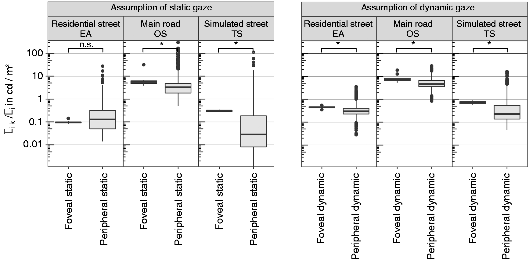

3.3. Omitting the upper quadrant of the spatial sampling pattern

In this analysis it has been assumed that all 68 sub-regions are equally relevant: this may not be the case. In particular the upper quadrant of a typical road scene is less likely to contain potential hazards (Figure 13). Hence the analysis was repeated but with the visual field reduced to exclude the upper quadrant.

Figure 13

A typical urban road scene when driving along a straight patch of a road.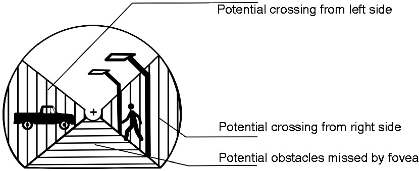

For the static assumption, the sampling pattern is centred within the scene and therefore the upper quadrant of the visual field of the sampling pattern matches the upper quadrant of the road scene.

For the dynamic assumption, omission of the upper quadrant becomes of particular significance if downward eye movement causes the road ahead (and hence the likely location of hazards) to fall into the upper quadrant. The road ahead begins to fall into the upper quadrant (for these flat roads) when the direction of gaze is 3° or more below the horizon: in the current eye tracking data, gaze direction was above this for 93% of the time.

The analyses of Sections 3.1 and 3.2 were repeated for this reduced field. Consider first the static versus dynamic comparison (Figure 14). For the peripheral field, the reduced field led to the same conclusions as did the whole peripheral sampling field (Figure 11).

Figure 14

Boxplot showing mean luminances in the peripheral field according to the assumption of static or dynamic visual field. In these data the upper quadrant of the visual field is omitted. These data are for the i = 10 images with k = 48 sub-areas each for the peripheral retinal locations (significant differences with p < 0.05 are indicated with *, n.s. otherwise). Note that the data of simulated street TS do not contain headlamps of one’s own vehicle.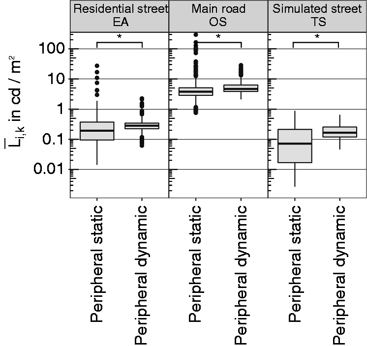

Consider next the foveal versus peripheral comparison (Figure 15). Here, there was a change to one conclusion: in residential street EA, the median of the foveal static field is lower than the median of peripheral static (p < 0.05, negligible effect size) whereas analysis with the whole field did not suggest a difference. This still contrasts with the five other analyses which suggest that the foveal field has a higher luminance than the peripheral field.

Figure 15

Boxplots comparing foveal retinal location to the peripheral retinal location based on the calculated mean luminances for i = 10 images for the foveal retinal location and for i = 10 images with k = 48 sub-areas each for the peripheral retinal locations, i.e. without the peripheral results of the upper quadrant (significant differences with p < 0.05 are indicated with *, n.s. otherwise). Note that the data of simulated street TS do not contain headlamps of one’s own vehicle.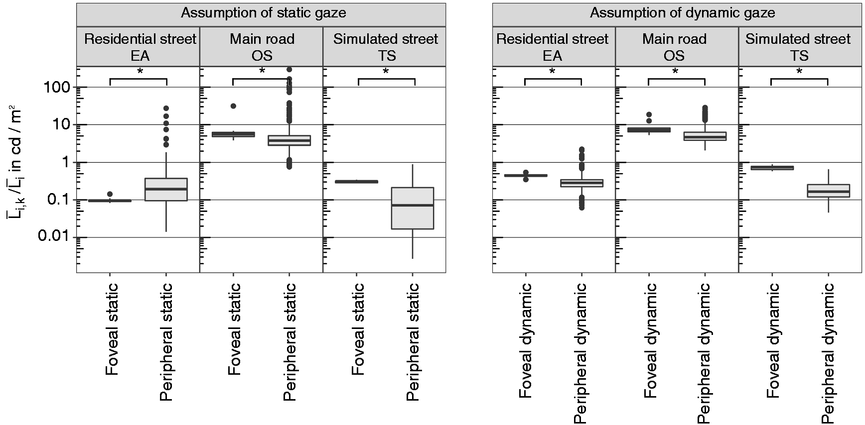

3.4. Application

For practical application, the interim recommendation of CIE JTC-1³⁶ proposes to use the average luminance of the design area (i.e. the luminance of the road surface as of CIE 140)⁵ as an estimator for the adaptation state. In another study it was identified that a 10° circle centred at the centre of lane at the horizon is a good estimator for that part of the visual field which encapsulates typical eye movements,¹⁷ and such a field has been examined in recent studies.^21,26

Figure 16 compares the mean luminances of the peripheral field, with both static and dynamic assumptions, to the mean luminance on the road and to the mean luminance within a horizon-centred 10° circle. The medians of the mean luminances within the 10° circle are higher than those estimated with the static or dynamic assumption in all six comparisons (p < 0.05, Wilcoxon rank sum test, small effect size). Consider next predictions of luminance using mean luminance of the road surface. In five of the six cases the road surface suggests a lower or equal luminance than do the spatial sampling based estimates (peripheral dynamic EA and OS, p < 0.05, small/negligible effect size; peripheral static EA, peripheral static OS and peripheral dynamic TS not suggested to be significantly different, p ≥ 0.12, negligible effect size, Wilcoxon rank sum test). In one case the road luminance leads to a higher predication of L_b (peripheral static TS, p < 0.05, small effect size, Wilcoxon rank sum test).

Figure 16

Boxplots comparing peripheral retinal location to the simplified methods (road/10° circle) based on the calculated mean luminances for i = 10 images for the simplified methods and for i = 10 images with k = 68 sub-areas each for the peripheral retinal locations (significant differences with p < 0.05 are indicated with *, n.s. otherwise). Note that the data of simulated street TS do not contain headlamps of one’s own vehicle.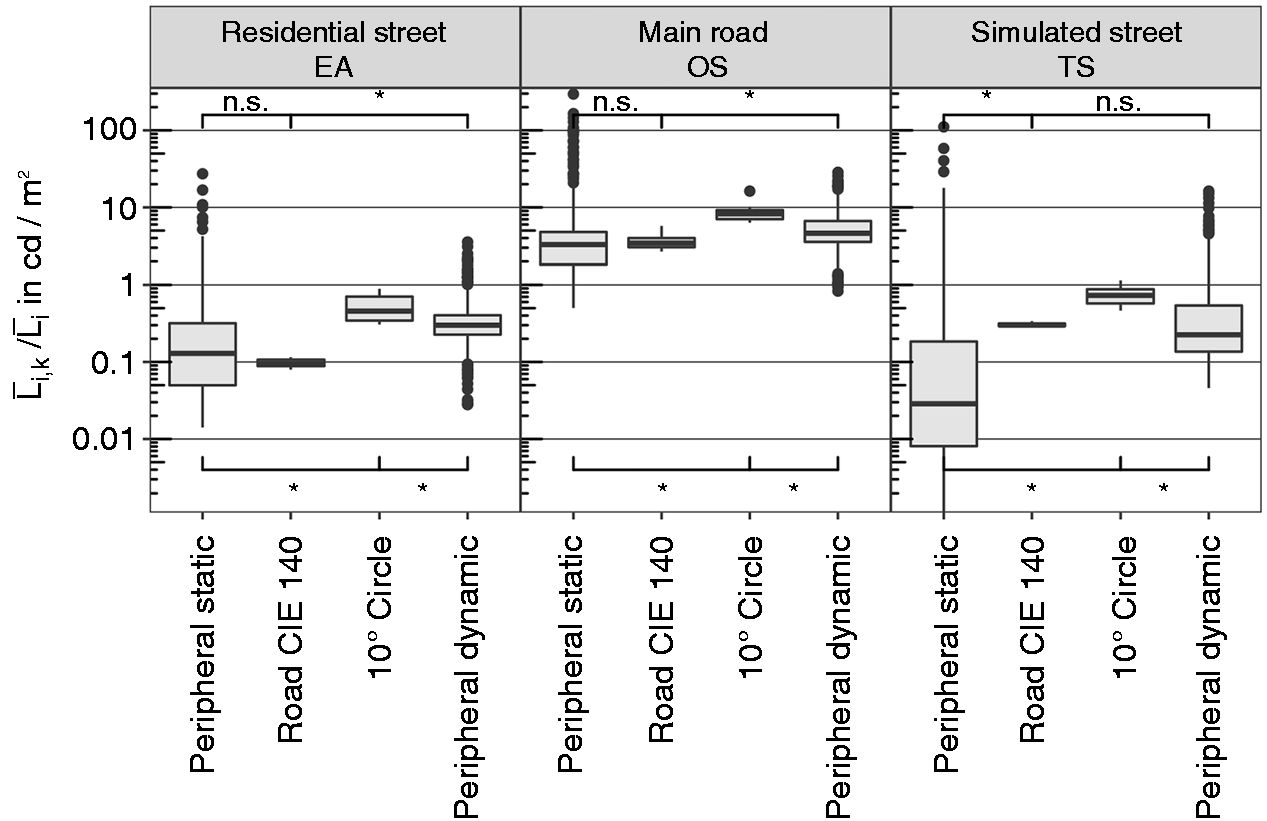

This analysis suggests that if a horizon-centred 10° circle is used to estimate L_b, it leads to a slightly high estimate of L_b; if instead the road surface luminance is used, this tends to lead to a slightly low estimate of L_b, which agrees with the findings of Uchida et al.¹⁶

Next, consider the impact of the visual field assumption for lighting design. This is illustrated here by determination of the mesopic enhancement factor (F_mes), the ratio of the mesopic luminance to the photopic luminance,³⁶ for two different spectra (Table 2). L_v was set to zero in the calculation of F_mes.

Table 2

Mesopic enhancement factor (F_mes) calculated for the three roads (EA, OS, TS) for four approaches to estimating background luminance, and for lighting of two SPDs (a white LED with S/P ratio = 1.71 and an HPS lamp with S/P ratio = 0.60).

Type of road	Method for estimating background luminance	Median luminance $(cd / m^{2})$	Mesopic enhancement factor (F_mes)
Type of road	Method for estimating background luminance	Median luminance $(cd / m^{2})$	S/P = 1.71	S/P = 0.60
Residential street EA	Road CIE 140	0.10	1.23	0.85
	Peripheral static	0.13	1.20	0.87
	Peripheral dynamic	0.30	1.14	0.91
	10° circle	0.46	1.12	0.93
Main road OS	Road CIE 140	3.43	1.02	0.99
	Peripheral static	3.29	1.02	0.99
	Peripheral dynamic	4.62	1.00	1.00
	10° circle	8.25	1.00	1.00
Simulated road TS	Road CIE 140	0.30	1.14	0.91
	Peripheral static	0.03	1.35	0.76
	Peripheral dynamic	0.23	1.16	0.90
	10° circle	0.73	1.09	0.94

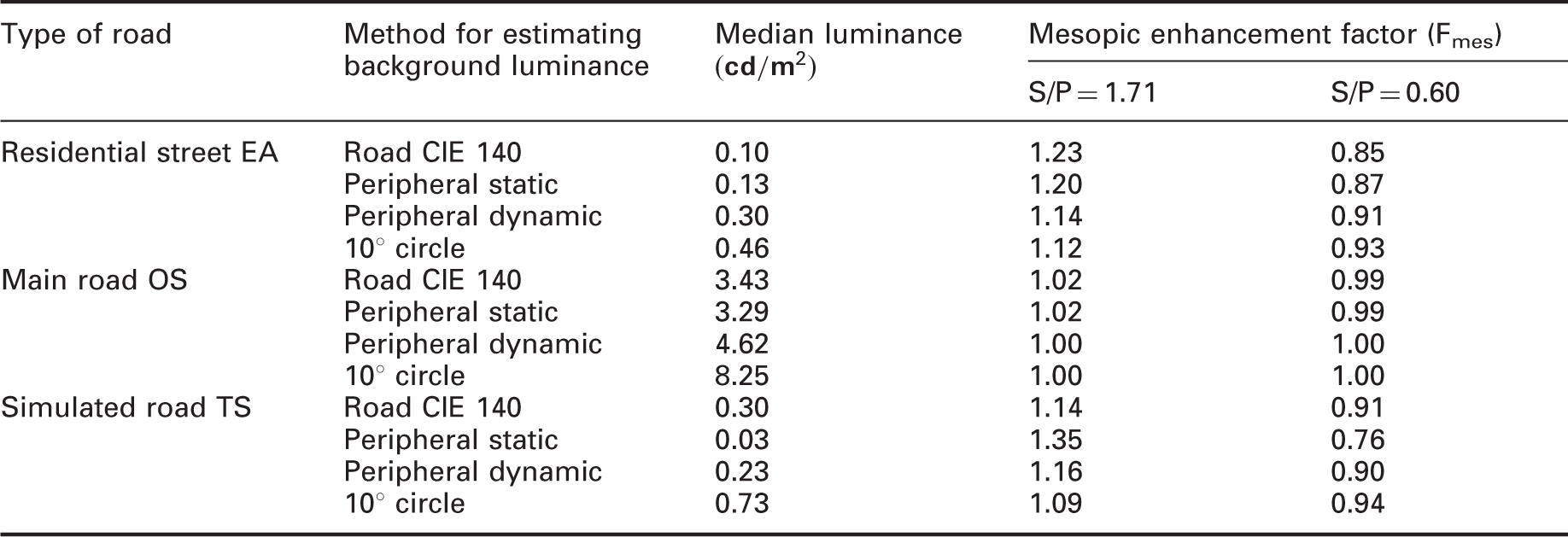
SPD: spectral power distribution; LED: light-emitting diode; HPS: high-pressure sodium; CIE: Commission Internationale de l’Eclairage.

For the residential road, where median luminances lie in the range of 0.1–0.5 cd/m², then the choice of the estimation method appears to influence F_mes. For example, the road surface approach having the lowest median luminance suggests that F_mes departs further from unity than do the other approaches. For the main road, however, the choice of method for estimating L_b has little effect on F_mes. This is because the main road, in this example, had a median luminance of >3 cd/m² which is close to the upper limit of the mesopic range (5 cd/m²). Note however that these are luminances higher than those typically recommended for main roads.⁴

4. Summary

The aim of this paper is to investigate assumptions made when estimating L_b, a component (alongside L_v due to glare) in estimates of a drivers’ state of adaptation. L_bs were therefore estimated using two approaches, these assuming static and dynamic visual fields. Dynamic eye movement was represented by the eye tracking records of a previous study.¹⁷ Scene luminances were represented by images taken at ten locations along each of three roads: a main road, a residential road and a simulated road. Luminances were determined for a 2° central field, representing the fovea. For the peripheral regions, the 20° circular region surround the fovea was divided into 68 individual 2° regions, and the mean luminance determined for each of these.

While standard approaches assume a static visual field, the driver experiences a dynamic field, due to movements of the vehicle and the driver’s head and eyes. Furthermore, the visual scene is complex, meaning it comprises a range of surfaces of different luminances rather than being a simple uniform field. The results (Figure 11) suggest that the L_b values estimated assuming a dynamic visual field are higher than those estimated assuming a static visual field, for both the foveal and peripheral regions. This finding did not change when omitting those parts of the visual field (the upper quadrant of the sampling pattern) considered less relevant for driving.

Within the estimated peripheral luminances, the range from minimum to maximum tends to be higher for the static assumption than for the dynamic assumption. Assuming that the duration of a fixation typically lies in the range of 0.35 s–0.8 s^37,38 and that the range of operation of the fast adaptation mechanisms (within 0.2 s, neural adaptation) seems to cover only 2 log units^7,15 this makes the dynamic assumption a more likely outcome when the gaze moves within the scene from fixation to fixation. Another way to see the dynamic approach is by looking at the weighted luminances as a likely outcome when considering the whole group of drivers. While the adaptation of a specific driver might be influenced by particularly different luminances (e.g. if the gaze rests at an extreme location), the adaptation of the majority of drivers; however, can be assumed to be influenced by the weighted mean luminance.

The L_b projected towards either foveal or peripheral regions may be of interest. It was found that the L_b values determined for the foveal region were significantly greater than those determined for the peripheral region, for both the static and dynamic assumptions. That finding changed in one case when omitting the upper quadrant of the sampling pattern. The peripheral luminances were, however, much more heterogeneous.

Compared with the L_b estimated for a dynamic peripheral field, a horizon-centred 10° circle led to a slightly higher estimate and the road surface luminance to a slightly lower estimate. As to whether this matters, that depends partly on where the L_b lies within the mesopic range. For lower luminances (the residential road in this study) then the different approaches to estimating L_b affect the estimate of F_mes. For higher luminances approaching the upper boundary of the mesopic range (the main road in this case) then there is little effect on F_mes. CIE TN 007³⁶ proposes use of the average luminance of the design area (i.e. road surface) to estimate L_b. The current work suggests this may lead to a lower estimate of L_b than that determined for a larger peripheral field, and that this may affect consideration of the mesopic effect at low luminances.

Footnotes

Declaration of conflicting interests

The authors declared no potential conflicts of interest with respect to the research, authorship, and/or publication of this article.

Funding

The authors disclosed receipt of the following financial support for the research, authorship, and/or publication of this article: Federal Ministry of Education and Research of Germany (13N10815).

References

Commission Internationale de l’Eclairage. CIE Publication 191. Recommended System for Mesopic Photometry Based on Visual Performance. Vienna: CIE, 2010.

Commission Internationale de l’Eclairage. CIE Publication 88. Guide for the Lighting of Road Tunnels and Underpasses. Vienna: CIE, 2004.

Commission Internationale de l’Eclairage. CIE Publication 31. Glare and Uniformity in Road Lighting Installations. Vienna: CIE, 1976.

Commission Internationale de l’Eclairage. CIE Publication 115. Recommendations for the Lighting of Roads for Motor and Pedestrian Traffic. Vienna: CIE, 2010.

Commission Internationale de l’Eclairage. CIE Publication 140. Road Lighting Calculations. Vienna: CIE, 2000.

Illuminating Engineering Society of North America. RP-8-14. Roadway Lighting. New York: IESNA, 2014.

Adrian

. Visibility of targets: model for calculation. Lighting Research and Technology 1989; 21: 181–188.

Narisada

. Visual perception in non-uniform fields. Journal of Light and Visual Environment 1992; 16: 81–88.

Stiles WS. The scattering theory of the effect of glare on the brightness difference threshold. Proceedings of the Royal Society London B 1929; 105: 131–146.

10.

Moon

Spencer

. The specification of foveal adaptation. Journal of the Optical Society of America 1943; 33: 444–456.

11.

Freiding

Eloholma

Ketomaki

Halonen

Walkey

Goodman

Alferdinck

Varady

Bodrogi

. Mesopic visual efficiency I: detection threshold measurements. Lighting Research and Technology 2007; 39: 319–334.

12.

Walkey

Orrevetelainen

Barbur

Halonen

Goodman

Alferdinck

Freiding

Szalmas

. Mesopic visual efficiency II: reaction time experiments. Lighting Research and Technology 2007; 39: 335–354.

13.

Varady

Freiding

Eloholma

Halonen

Walkey

Goodman

Alferdinck

. Mesopic visual efficiency III: discrimination threshold measurements. Lighting Research and Technology 2007; 39: 355–364.

14.

Wördenweber

Wallaschek

Boyce

Hoffman

. Automotive Lighting and Human Vision, Berlin: Springer, 2007.

15.

Boyce

. Human Factors in Lighting, 3rd edition. Boca Raton, FL: CRC Press, 2014.

16.

Uchida

Ayama

Akashi

Hara

Kitano

Kodaira

Sakai

. Adaptation luminance simulation for CIE mesopic photometry system implementation. Lighting Research and Technology 2016; 48: 14–25.

17.

Winter

Fotios

Völker

. Gaze direction when driving after dark on main and residential roads: where is the dominant location? Lighting Research and Technology 2017; 49: 574–585.

18.

Liversedge

Gilchrist

Everling

. The Oxford Handbook of Eye Movements. EBSCO ebook academic collection. Oxford: Oxford University Press, 2011.

19.

Land

. Eye movements and the control of actions in everyday life. Progress in Retinal and Eye Research 2006, 25; pp. 296–324.

20.

Rothkopf

Ballard

Hayhoe

. Task and context determine where you look. Journal of Vision 2007, 7: pp. 1–20.

21.

Cengiz

Kotkanen

Puolakka

Lappi

Lehtonen

Halonen

Summala

. Combined eye-tracking and luminance measurements when driving on a rural road: towards determining of mesopic adaptation luminance. Lighting Research and Technology 2014; 46: 676–694.

22.

Kountouriotis

Spyridakos

Carsten

OMJ

Merat

. Identifying cognitive distraction using steering wheel reversal rates. Accident Analysis and Prevention 2016; 96: 39–45.

23.

Crundall

Chapman

Phelps

Underwood

. Eye movements and hazard perception in police pursuit and emergency response driving. Journal of Experimental Psychology: Applied 2003; 9: 163–174.

24.

Adrian

. Adaptation luminance when approaching a tunnel in daytime. Lighting Research and Technology 1987; 19: 73–79.

25.

Völker S. Hell- und Kontrastempfindung - ein Beitrag zur Entwicklung von Zielfunktionen für die Auslegung von Kraftfahrzeug-Scheinwerfern. [Brightness and contrast perception – a contribution for developing objective functions for designing motor vehicle headlights]. Habilitation, Universität Paderborn, Paderborn, Germany, 2006.

26.

Maksimainen

Puolakka

Tetri

Halonen

. Veiling luminance and visual adaptation field in mesopic photometry. Lighting Research and Technology 2017; 49: 743–762.

27.

Uchida

Ohno

. Defining the visual adaptation field for mesopic photometry: does surrounding luminance affect peripheral adaptation? Lighting Research and Technology 2014; 46: 520–533.

28.

Cengiz

Puolakka

Halonen

. Reaction time measurements under mesopic light levels: towards estimation of the visual adaptation field. Lighting Research and Technology 2014; 47: 828–844.

29.

Cengiz

Maksimainen

Puolakka

Halonen

. Contrast threshold measurements of peripheral targets in night-time driving images. Lighting Research and Technology 2016; 48: 491–501.

30.

Winter

Fotios

Völker

. The effects of glare and inhomogeneous visual fields on contrast detection in the context of driving. Lighting Research and Technology First published 7 October 2016 DOI: 10.1177/1477153516672719.

31.

Winter J, Buschmann S, Franke R. RoadRad: a Radiance Road Lighting Simulation Framework. 2003, Available from: https://github.com/fglichttechnik/Radiance-RoadLighting-Simulation-Framework.

32.

Wang

Stein

Gao

. A review of spatial sampling. Spatial Statistics 2012; 2: 1–14.

33.

Rosenthal

. Cooper

Hedges

. Parametric Measures of Effect Size, New York: Russell Sage Foundation, 1994, pp. 231–244.

34.

Pallant

. SPSS Survival Manual: a Step by Step Guide to Data Analysis using SPSS, Sydney: Australia: Allen & Unwin, 2010.

35.

Cohen

. A power primer. Psychological Bulletin 1992; 112: 155–159.

36.

Commission Internationale de l’Eclairage. TN 007:2017. Interim Recommendation for Practical Application of the CIE system for Mesopic Photometry in Outdoor Lighting. Vienna: CIE, 2017.

37.

Chapman

Underwood

. Visual search of driving situations: danger and experience. Perception 1998; 27: 951–964.

38.

Underwood

Chapman

Bowden

Crundall

. Visual search while driving: skill and awareness during inspection of the scene. Transportation Research Part F: Traffic Psychology and Behaviour 2002; 5: 87–97.

The effect of assuming static or dynamic gaze behaviour on the estimated background luminance of drivers

Abstract

1. Introduction

2.Method

2.1. Luminance data

2.2. Estimation of foveal Lb based on eye movement

2.3. Estimation of peripheral Lb

2.3.1. Spatial sampling of the visual field

2.3.2. Static assumption

2.3.3. Dynamic assumption

3. Results

3.1. Static versus dynamic

3.2. Foveal versus peripheral

3.3. Omitting the upper quadrant of the spatial sampling pattern

3.4. Application

4. Summary

Footnotes

Declaration of conflicting interests

Funding

References

2.2. Estimation of foveal L_b based on eye movement

2.3. Estimation of peripheral L_b