Using spectral sensors to determine photosynthetic photon flux density in daylight

Abstract

Precise determination of the photosynthetic photon flux density (PPFD) is important for illumination in modern horticultural systems. This paper presents two methods to calculate the PPFD of daylight spectra using low cost optic sensors. The first method uses the spectral sensitivity functions of spectral sensors to recreate the quantum sensitivity curve of quantum sensors. Two sets of spectral sensitivity functions are compared. The second method calculates the PPFD based on the calculated correlated colour temperature and a spectral reconstruction using the CIE daylight model. It is demonstrated that all methods offer a useful estimation of the PPFD with correspondingly similar daylight spectra, but the supposedly simpler method, which is based on weighting of the individual channels, is more stable against deviations from the CIE daylight model.

1. Introduction

Plant growth in greenhouses is affected by temperature, humidity, nutrient supply, water supply and light. In modern horticulture, growers are increasingly supported by technology to handle these parameters; for example, decision making on irrigation is provided by sensors.¹ Regular measurement of nutrients in the substrate or nutrient solution is moreover already part of the repertoire of a modern grower.

To take control of the light environment, light affecting plant growth needs to be measured. According to McCree in 1972,² radiation in the range from 400 nm to 700 nm is used for photosynthesis and therefore defined as photosynthetic active radiation (PAR). This range has been used for a long time but may be extended in the future to include far red radiation, as proposed by Zhen et al. ³ Inside the PAR range, all photons are summed up, without further weighting.

Growers and farmers are measuring the photosynthetic active photon flux density (PPFD) in µmol m⁻² s⁻¹, which indicates how many photons in the spectral range of PAR radiation are received per area and time unit. By continuously recording the PPFD, it is possible to determine the light sum of an area element over the entire day, referred to as the daily light integral (DLI). Different crops have different needs regarding the DLI. An estimation of the DLI using prediction models based on the solar radiation was proposed by Albright et al. ⁴

If the natural sunlight is not sufficient, supplemental lighting in greenhouses is used to achieve a constant PPFD, where a control loop is built using sensors to measure PPFD.^5–7 Previous works have used different approaches to measure PPFD.^8–19 Summed up, it can be done with several techniques, as stated by Ross and Sulev²⁰ using: (1) spectroradiometers; (2) pyranometers covered with hemispherical glass filters; or (3) sensors based on silicon photodiodes (quantum sensors).

Using spectrometers returns information about the spectral composition of the light; however, it is too expensive for broad applications in field. Pyranometers are used to measure sun radiation, including the IR-range. Today, quantum sensors are mostly used in the field of horticultural applications. Those are constructed using a photodiode to measure irradiance, while the spectrum is weighted according to the photon energy using an optical filter set.

Barnes et al. demonstrated that depending on the spectrum of the radiation source, as well as on the spectral response of the quantum sensor, the accuracy can vary, while broad light sources are most accurate.²¹ Blonquist et al. as well as an experiment performed by LI-COR measured errors of more than 30 % by testing different sensors in a variety of light sources.^22,23 Quantum sensors are not able to attain spectral information, and having this information could be beneficial.

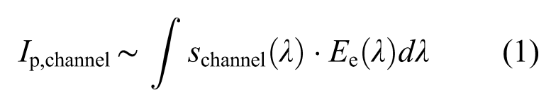
Recent work introduced spectral sensors as a promising tool to measure PPFD.^24,25 Spectral sensors are an array of photodiodes, each one coated with different optical bandpasses. For one diode-filter component, the digital output corresponds to the integral of the sensor spectral sensitivity s _channel(λ), which is dependent on the optical filter and the used semiconductor. The sensor output is proportional to the sensitivity and the spectral irradiance Ee(λ)

I_{p, channel} \sim \int s_{channel} (λ) \cdot E_{e} (λ) d λ

(1)

In dependence of the amount of different photodiode-filter combinations (channels), the information about the spectral composition of the irradiance varies. Usually, the centre-wavelength of the optical filters is distributed over the visible range. Due to the sensitivity of silicon in the infrared region, measurement in this region is possible, too.

Depending on the application, optical filters are used to customise the sensitivity function to enable: (1) spectral measurements, (2) a fit to the colour response curves of the eye, (3) a fit to the luminous efficiency function for photopic vision V(λ), and (4) a fit to calculate R-G-B-components. None of these filters allows a direct measurement of the PPFD, but those filters can be used to determine information about the spectrum. This enables the calculation of a conversion factor to calculate PPFD from measured irradiance.

The focus of this work is on the error of different methods to determine this conversion factor. Future works can benefit from this investigation by choosing an appropriate method for individual illumination case.

2. Experimental details and methods

In this work, several optical sensors are used. A multi-channel spectral sensor AS7341 from AMS with 8 channels in the range between 400 and 700 nm (sensor 1),²⁶ an R-G-B sensor TCS3472 from AMS with three channels representing colour metrics (sensor 2)²⁷ and a colour sensor AS7264n from AMS, measuring tri-stimulus values (sensor 3) (Table 1).²⁸

Table 1

Overview of the sensors used in this work

	Sensor	Channels
Sensor 1	AS7341	8 optical + 3 extra
Sensor 2	TCS3472	X,Y,Z
Sensor 3	AS7264n	R,G,B

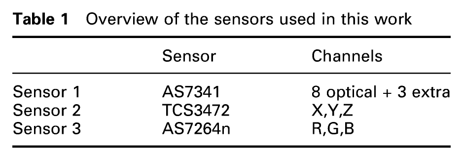
Two methods are used: method 1 uses a reduced PAR-weighting function to calculate PPFD, and method 2 uses the CIE daylight model. Method 1 is applied to sensors 1 and 2, while method 2 is applied to sensors 2 and 3. Characteristics of all sensors are used to calculate their theoretical ability to measure the PFPD under a daylight spectrum. Therefore, the sensors response to different monochromatic light sources is determined using the setup in Figure 1.

Figure 1

The set-up of the measurement and determination for the sensitivity curves of spectral sensors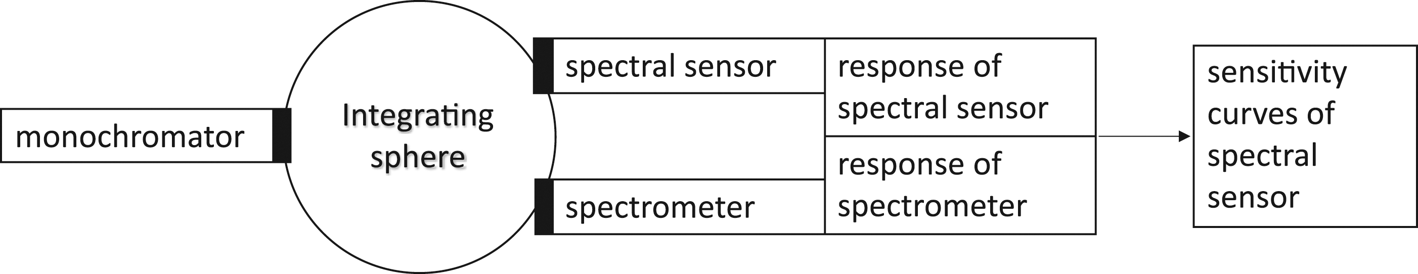

In this setup, monochromatic light provided from a Xenon light source together with a LOT MSH-300 monochromator enters an integrating sphere (6 inch diameter), where the spectral sensor and a spectrometer (Spectro 320 scanning spectrometer from Instrument Systems) with a resolution smaller than that of the spectral sensor are mounted to. The spectrometer serves as a reference measurement for the characterisation. 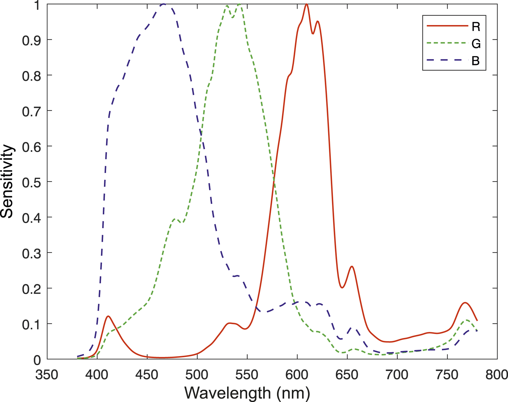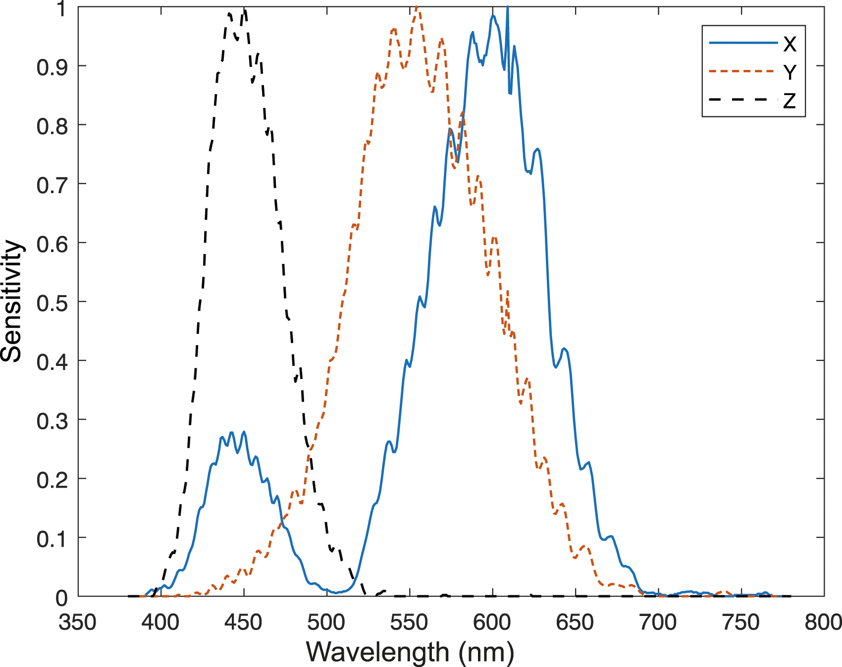Sweeping the centre-wavelength of the entering quasi-monochromatic light enables the calculation of the spectral sensors sensitivity curves by dividing the response of the sensor through the spectrometer one, which is known as the simple estimates procedure.^29,30 With this setup, the sensitivity curves for sensor 1 are illustrated in Figure 2, for sensor 2 in Figure 3 and for sensor 3 in Figure 4

Figure 2

Sensitivity curves of the multi-channel spectral sensor (sensor 1). S1 to S8 sorted by increasing peak wavelength

Figure 3

Sensitivity curves of the R-G-B sensor (sensor 2)

Figure 4

Sensitivity curves of the X,Y,Z sensor (sensor 3)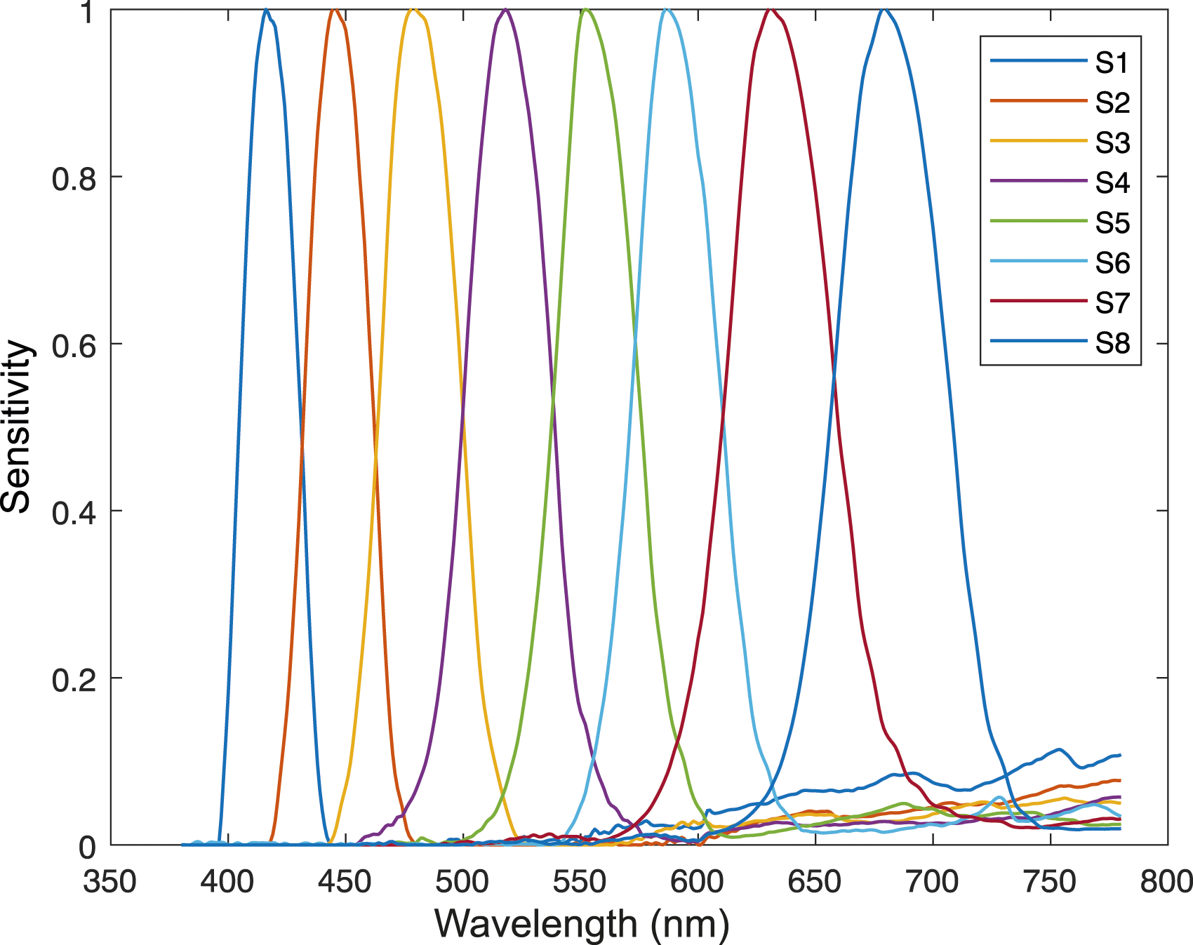

Using these sensitivity curves, two methods are presented in the following to calculate the PPFD.

2.1 Calculating PPFD from spectral irradiance

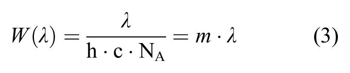
To calculate PPFD (E _p,PAR), analogue to the V(λ) curve, a weighting function is needed to transform the energy-based quantity to a quantum-based one

E_{p, PAR} = \int_{- \infty}^{\infty} E_{e, PAR} (λ) \cdot W (λ) \cdot d λ

(2)

where W(λ) is a function to weight the spectral irradiance according to the energy content of photons at the specific wavelength λ. To eliminate the contribution of radiation outside the PAR range, the integral is limited to the range between 400 nm and 700 nm. In the next step, to estimate W(λ), the energy-based quantity W m⁻² needs to be converted to the quantity µmol m⁻² s⁻¹. This is done via Planck’s quantum of action h (6.6261×10⁻³⁴ J s), Avogadro constant N_A (6.0221×10²³ mol⁻¹) and speed of light c (299 792 458 m s⁻¹)

W (λ) = \frac{λ}{h \cdot c \cdot N_{A}} = m \cdot λ

(3)

The weighting function is linearly dependent on wavelength λ with a slope m, defined by the combination of the constants h, c and N_A. A plot of the weighting function is illustrated in Figure 5

E_{p, PAR} = \int_{400 nm}^{700 nm} E_{e} (λ) \cdot rect (λ) \cdot \frac{λ}{h \cdot c \cdot N_{A}} d λ

(4)

Figure 5

Photon flux density per Watt in dependence of the wavelength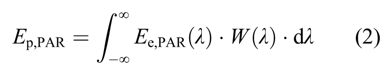

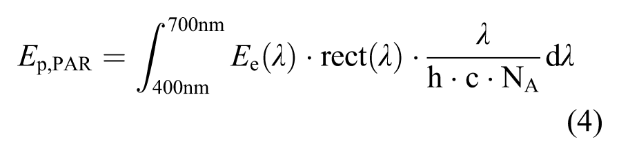
Equation (4) can be rewritten as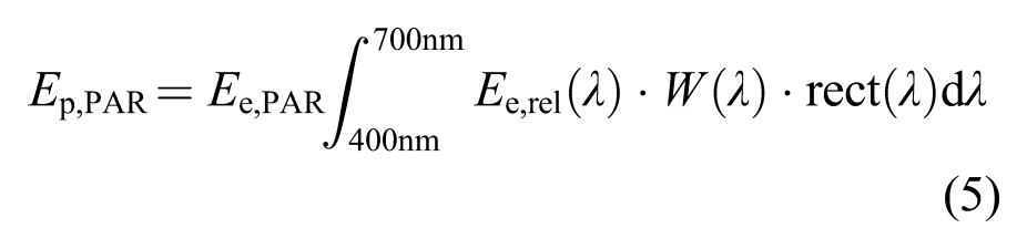

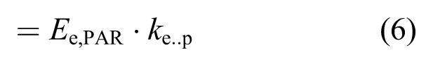
\begin{array}{l} E_{p, PAR} & = E_{e, PAR} \int_{400 nm}^{700 nm} E_{e, rel} (λ) \cdot W (λ) \cdot rect (λ) d λ \end{array}

(5)

= E_{e, PAR} \cdot k_{e .. p}

(6)

where E _e,PAR is the absolute optical energy in the PAR spectral range, E _e,rel(λ) the relative spectral distribution of the energy and

k_{e .. p}

a spectral distribution dependent factor to calculate E _p,PAR from an integral measurement of E _e,PAR with a known spectral distribution.

For a precise determination of E _e,PAR, the critical part is the determination of $k_{e .. p}$ , as this can only be done using information about the spectral distribution. This work is investigating two methods using three different spectral sensors to determine factor $k_{e .. p}$ for future investigations on estimating E _e,PAR in daylight.

2.2 Method 1: Determination based on reduced PAR-weighting functions

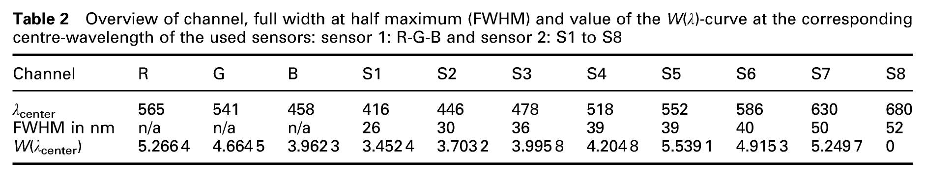
The first method to approximate E _p,PAR using spectral sensors is based on the sensitivities of the channels. Thus, the W(λ) function is simulated using the sensitivities and additional weights a _n, which depend on the value of the W(λ) function at the centre-wavelength, and the sum of these weighted channels is taken as the PPFD.

For the simulation, the weights are determined from the W(λ)-curve at the corresponding centre wavelength and are displayed in Table 2. Because of normalised incidence spectra used in this calculation, all a _n were set to 1. In a first approach, a ₈ was set to 0.75 for channel S8 as almost three quarters of its sensitivity are in the PAR-range (≤700 nm). However, with a ₈ set to zero, the variance was lowest.

Table 2

Overview of channel, full width at half maximum (FWHM) and value of the W(λ)-curve at the corresponding centre-wavelength of the used sensors: sensor 1: R-G-B and sensor 2: S1 to S8

Channel	R	G	B	S1	S2	S3	S4	S5	S6	S7	S8
λ _center	565	541	458	416	446	478	518	552	586	630	680
FWHM in nm	n/a	n/a	n/a	26	30	36	39	39	40	50	52
W(λ _center)	5.266 4	4.664 5	3.962 3	3.452 4	3.703 2	3.995 8	4.204 8	5.539 1	4.915 3	5.249 7	0

Factor $k_{e .. p}$ is determined using the following equation with different relative daylight spectra

k_{e .. p} = \sum_{i = 1}^{n} W (λ_{center, i}) \cdot a_{n} \cdot \int s_{channel, i} (λ) \cdot E_{e, rel} (λ) d λ

(7)

where the channel number n is 8 for sensor 1 and 3 for sensor 2. Method 1 is applied to sensor 1 and sensor 2, as those have narrow-band optical filters.

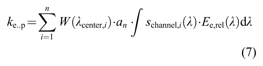
2.3 Method 2: Determination based on the CIE daylight model

The second method uses an approach based on the correlated colour temperature (CCT) and a reconstruction of the spectrum using the CIE daylight model.

The CIE daylight model³¹ is a linear combination of different vectors describing the phases of daylight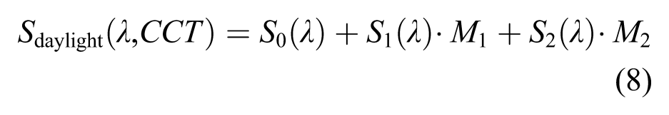

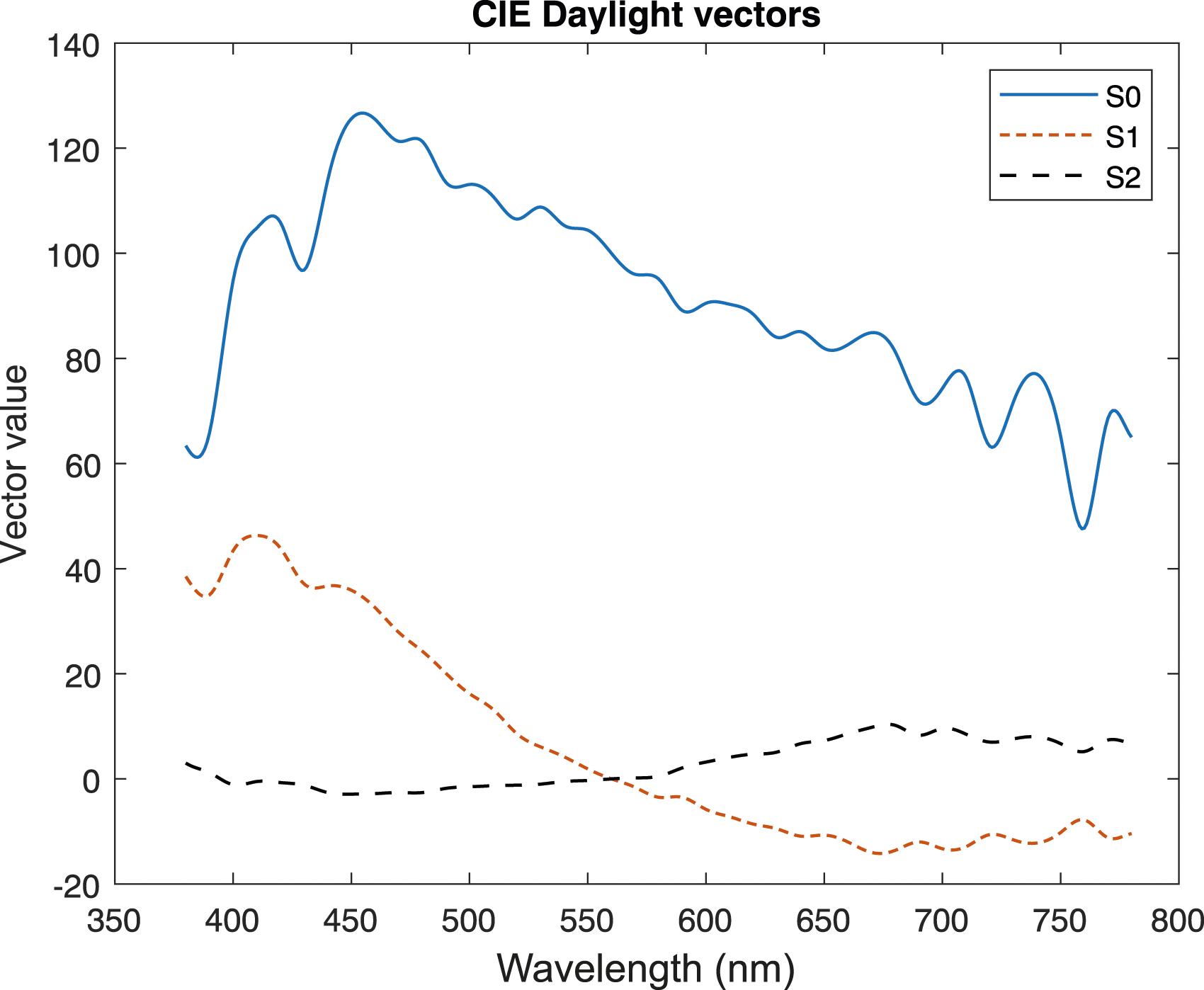
S_{daylight} (λ, C C T) = S_{0} (λ) + S_{1} (λ) \cdot M_{1} + S_{2} (λ) \cdot M_{2}

(8)

These basic curves S ₀(λ), S ₁(λ) and S ₂(λ) are illustrated in Figure 6.

Figure 6

The basic curves S0(λ), S1(λ), S2(λ) of CIE daylight model³¹

To apply the daylight model, the correlated colour temperature (CCT) of the spectrum needs to be determined from the sensor values. For sensor 3, CCT can be obtained by transforming the X,Y tristimulus values to x,y colour coordinates and applying the formula from McCamy.³²

This can furthermore be applied for sensor 2, but first, the R-G-B sensor values need to be transformed to X,Y,Z. For this purpose, a transformation matrix is empirically calculated, which allows transformation of the sensor responses. This transformation matrix is calculated using the optimisation algorithm ‘fminsearch’ in Matlab. The optimisation constraint is a low Δ_Eu′v′ between the input spectra and the calculated X,Y,Z values of the R-G-B sensor. With a determination constraint of Δ_Eu′v′ ≤ 0.003, the transformation-matrix results in the matrix given in equation (9)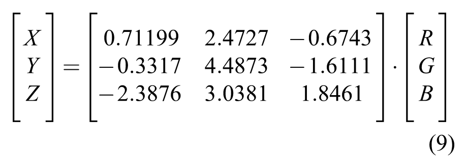

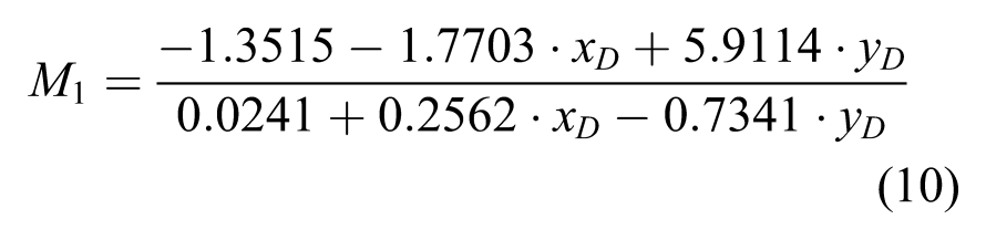
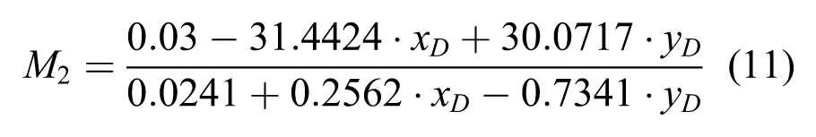
[\begin{matrix} X \\ Y \\ Z \end{matrix}] = [\begin{matrix} 0.71199 & 2.4727 & - 0.6743 \\ - 0.3317 & 4.4873 & - 1.6111 \\ - 2.3876 & 3.0381 & 1.8461 \end{matrix}] \cdot [\begin{matrix} R \\ G \\ B \end{matrix}]

(9)

In a second step, factors M ₁ and M ₂ from equation (8), which are based on the chromaticity coordinates x _D and y _D of the daylight phase are computed³¹

M_{1} = \frac{- 1.3515 - 1.7703 \cdot x_{D} + 5.9114 \cdot y_{D}}{0.0241 + 0.2562 \cdot x_{D} - 0.7341 \cdot y_{D}}

(10)

M_{2} = \frac{0.03 - 31.4424 \cdot x_{D} + 30.0717 \cdot y_{D}}{0.0241 + 0.2562 \cdot x_{D} - 0.7341 \cdot y_{D}}

(11)

The chromaticity coordinates are determined as follows, for CCT between 5000 K and 7000 K.

And for CCT above 7000 K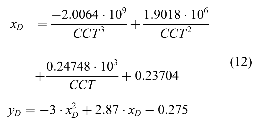

\begin{array}{l} \begin{array}{l} x_{D} & = \frac{- 2.0064 \cdot 10^{9}}{C C T^{3}} + \frac{1.9018 \cdot 10^{6}}{C C T^{2}} \\ + \frac{0.24748 \cdot 10^{3}}{C C T} + 0.23704 \end{array} \\ y_{D} = - 3 \cdot x_{D}^{2} + 2.87 \cdot x_{D} - 0.275 \end{array}

(12)

After calculation of those factors, the daylight spectrum to the corresponding CCT is determined using equation (8). Using this spectrum S _daylight (λ, CCT) and equation (4) leads to factor 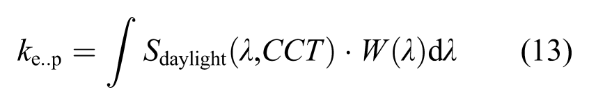$k_{e .. p}$

k_{e .. p} = \int S_{daylight} (λ, C C T) \cdot W (λ) d λ

(13)

2.4 Determination of the error

To calculate the error of factor 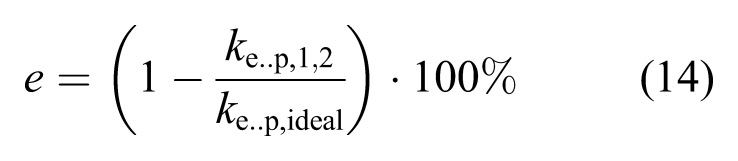$k_{e .. p}$ between an ideal quantum sensor and the sensors used in this work, the following equation is applied

e = (1 - \frac{k_{e .. p, 1,2}}{k_{e .. p, ideal}}) \cdot 100 %

(14)

where k _e..p,1,2 is the factor of the sensor using method 1 or 2 and k _e..p,ideal for the ideal one, calculated from the spectrum.

3. Results

Various test datasets were used to calculate the accuracy of the methods. The set of test spectra contains daylight-spectra calculated by the CIE-Method and real-world measurements under clear (19.08.2020, Darmstadt N 49.87, E 8.65, Germany) and cloudy (23.09.2020, Darmstadt N 49.87, E 8.65, Germany) sky, taken horizontally by a handheld spectrometer (CSS-45 Gigahertz-Optik). 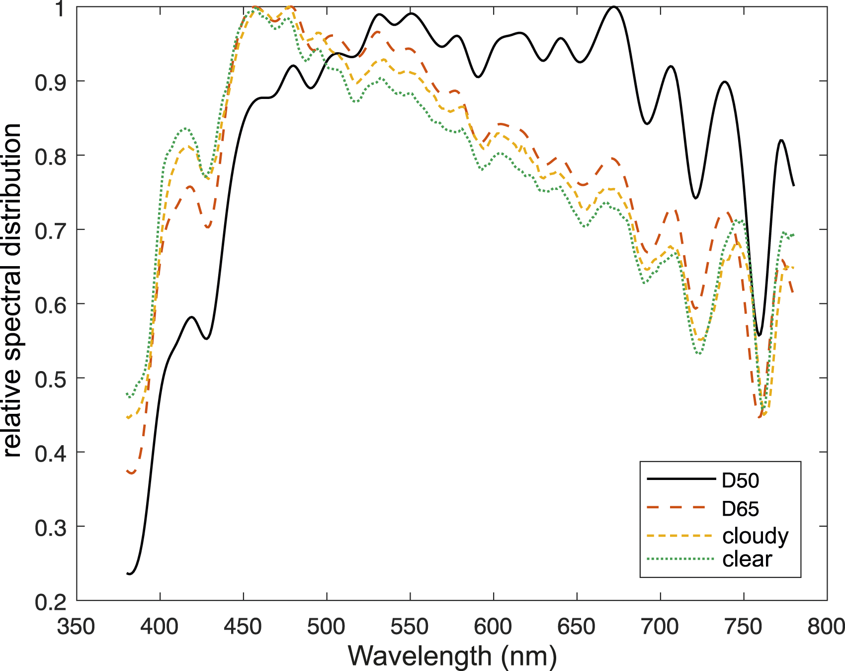A set of 215 spectra was obtained, split into 131 training spectra and 84 test spectra.³³ CCT of the spectra ranges from 5000 K to 16 000 K, calculated using the method by McCamy.³² Figure 7 displays the distribution of the used CCTs. Most spectra were in the range between 5000 K and 6000 K, with most spectra above 6000 K being calculated using the CIE-daylight model. Due to differences between clear and cloudy sky as well as to the CIE-daylight distribution, it is important to mix these data for training and test data to train this system for more than one daylight-condition. Mixing these sets leads to a variation of the incidence spectra, which causes a more robust calculation when applying the trained model. To illustrate the differences in the spectra, Figure 8 shows some spectra of the clear and cloudy sky as well as D65 and D50 daylight spectra.

Figure 7

Distribution of the test dataset CCT

Figure 8

Relative spectral distribution of D50 and D65 daylight spectra and two examples of diffuse and direct measured spectra at clear and cloudy sky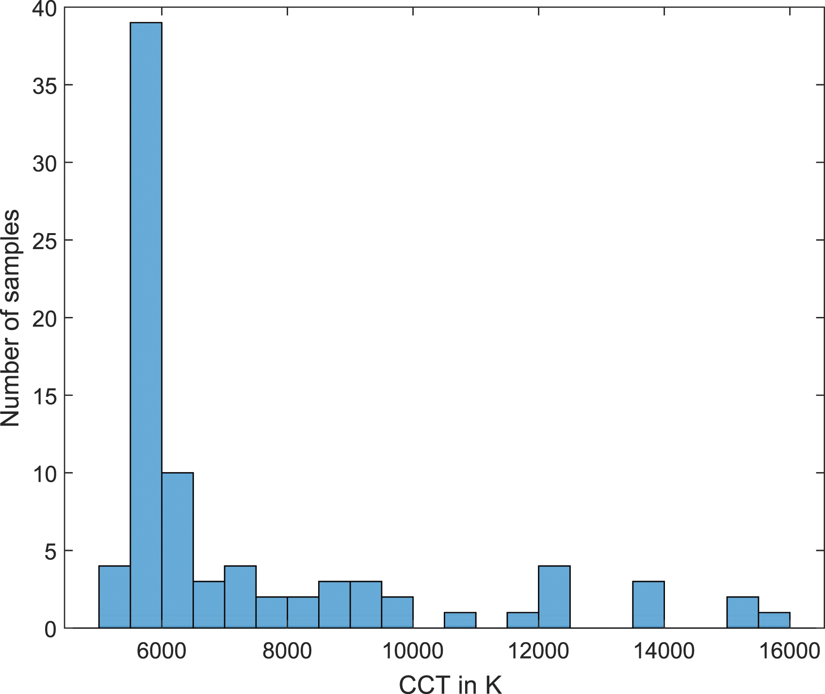

Errors in the following sections were calculated using equation (14). For sections 3.1 and 3.2, the training dataset was used, for section 3.3 the test one.

3.1 Error using method 1

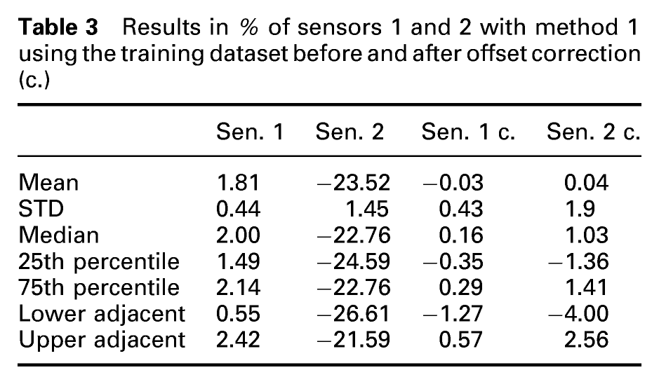
The results for method 1 are illustrated in Figure 9. The horizontal line shows the median and the whiskers represent the 95% confidence interval. The outliers are marked with +. Sensor 1, using the 8-channel spectral sensor, has a mean error of 1.81 % compared to the one of sensor 2 with an underestimation of −23.52 %. The over- or underestimation of the PPFD with a relatively small variance allows an offset correction of the calculation. The overestimation of sensor 1 is probably due to the overlapping of the individual channels and the rising sensitivity in longer wavelength (see Figure 2). The underestimation of sensor 2 is due to the low number of sampling points.

Figure 9

Results of both sensors and methods using the training spectra before and after offset correction (labelled with ‘c.’). In this graph and also Figures 10 and 11, the horizontal line shows the median, the whiskers represent the 95% confidence interval, and outliers are marked with +.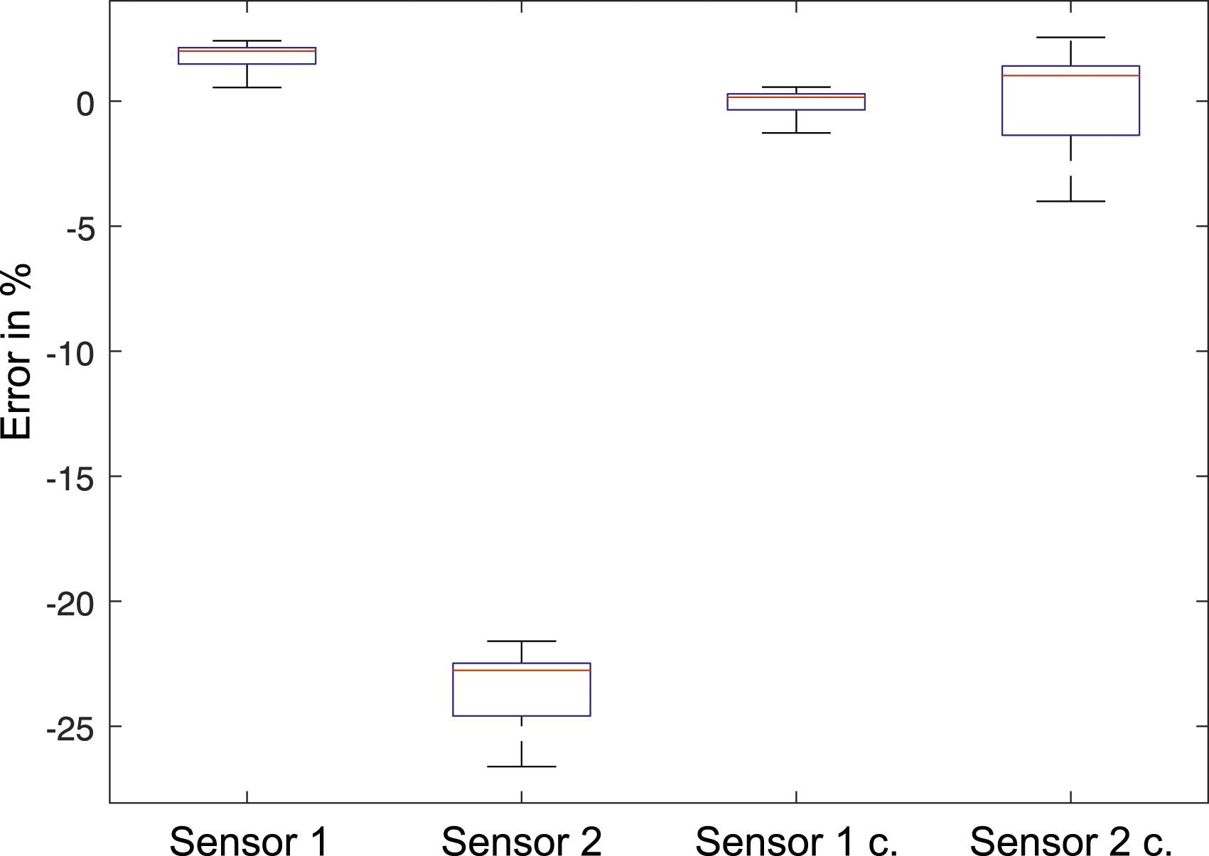

Mean value is used as an offset factor and calculations are repeated. This leads to a decrease in the mean error, with an underestimation of 0.03 % for sensor 1, respectively, an overestimation of 0.04 % for sensor 2. The error using sensor 2 is reduced to almost the same as sensor 1. Sensor 1 is due to the higher amount of measuring points (8 compared to 3 for sensor 2), more stable against spectral variation, which results in a lower standard deviation (Table 3).

Table 3

Results in % of sensors 1 and 2 with method 1 using the training dataset before and after offset correction (c.)

	Sen. 1	Sen. 2	Sen. 1 c.	Sen. 2 c.
Mean	1.81	−23.52	−0.03	0.04
STD	0.44	1.45	0.43	1.9
Median	2.00	−22.76	0.16	1.03
25th percentile	1.49	−24.59	−0.35	−1.36
75th percentile	2.14	−22.76	0.29	1.41
Lower adjacent	0.55	−26.61	−1.27	−4.00
Upper adjacent	2.42	−21.59	0.57	2.56

3.2 Error using method 2

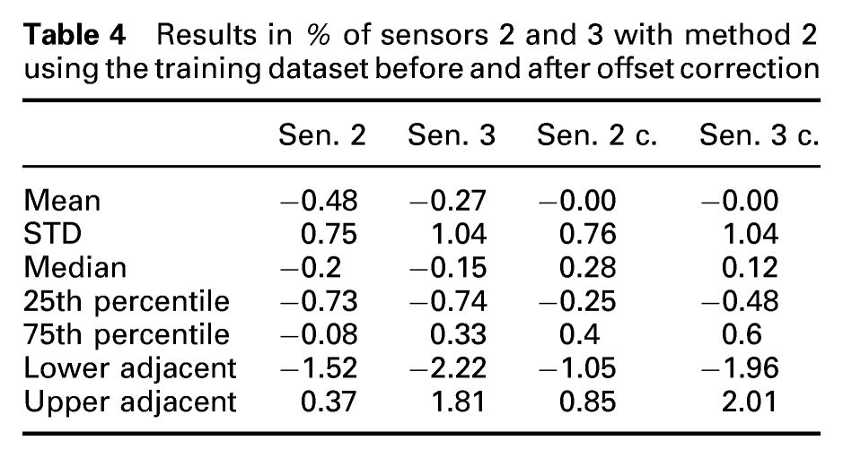
Using the spectral reconstruction method with the CIE-daylight model leads to a lower mean error with the use of sensor 2 (R-G-B) and sensor 3 (X,Y,Z) compared to method 1 (see Figure 10). Mean error for sensors 2 and 3 is nearly the same, with −0.48 % and −0.27 %, respectively. After considering the offset, mean error is decreased to zero. Using this method, errors with and without offset correction are smaller than using method 1. Offset is set to be the mean of the error over all training spectra (Table 4).

Figure 10

Results of both sensors and methods using the training dataset after offset correction (c.)

Table 4

Results in % of sensors 2 and 3 with method 2 using the training dataset before and after offset correction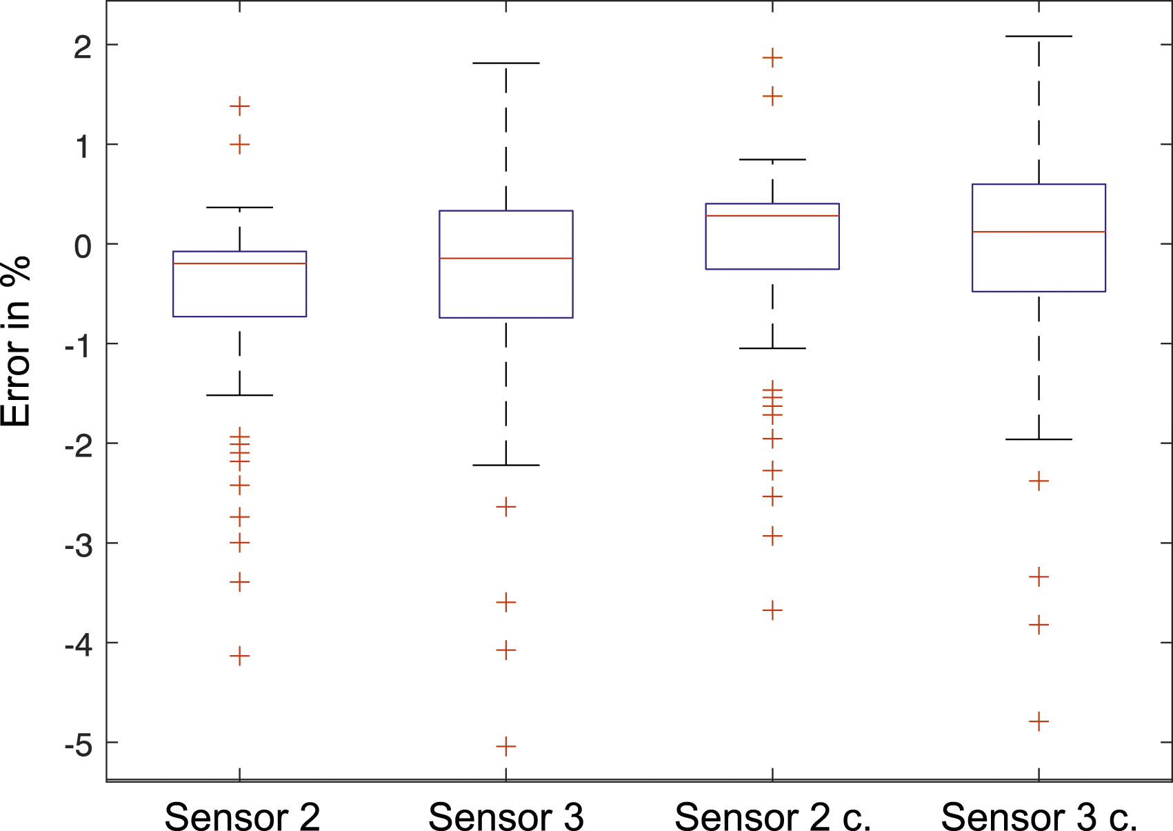

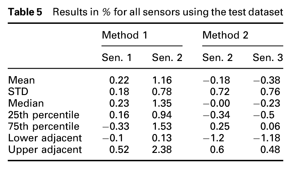
	Sen. 2	Sen. 3	Sen. 2 c.	Sen. 3 c.
Mean	−0.48	−0.27	−0.00	−0.00
STD	0.75	1.04	0.76	1.04
Median	−0.2	−0.15	0.28	0.12
25th percentile	−0.73	−0.74	−0.25	−0.48
75th percentile	−0.08	0.33	0.4	0.6
Lower adjacent	−1.52	−2.22	−1.05	−1.96
Upper adjacent	0.37	1.81	0.85	2.01

3.3 Errors using test spectra dataset

After training and determination of the offset factors using the training dataset, all methods are applied to the test dataset. The results are displayed in Figure 11, and error values are in Table 5. With the test dataset, method 1 in combination with sensor 1 leads to an error with a low standard deviation. Mean error for method 1 using sensor 1 and method 2 using sensor 2, respectively 3, is similar, but with a larger standard deviation. Largest error occurs with sensor 2, using method 1, which was the same case using method 1 without offset correction (see Table 3).

Figure 11

Results for all sensors using the test dataset. The applied offset correction was determined using the training dataset

Table 5

Results in % for all sensors using the test dataset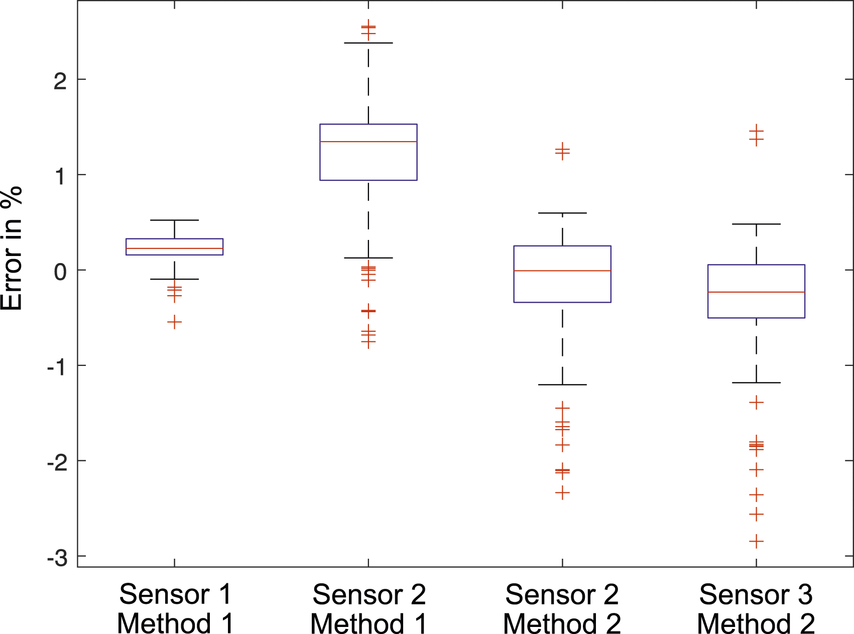

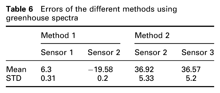
	Method 1		Method 2
	Sen. 1	Sen. 2	Sen. 2	Sen. 3
Mean	0.22	1.16	−0.18	−0.38
STD	0.18	0.78	0.72	0.76
Median	0.23	1.35	−0.00	−0.23
25th percentile	0.16	0.94	−0.34	−0.5
75th percentile	−0.33	1.53	0.25	0.06
Lower adjacent	−0.1	0.13	−1.2	−1.18
Upper adjacent	0.52	2.38	0.6	0.48

3.4 Errors using greenhouse spectra

After characterising the methods using daylight spectra, a dataset of spectra measured under a greenhouse roof without artificial lighting (horizontal twin-wall sheets) is evaluated. In total, 810 spectra were used for this test, measured between July and September 2020 near Darmstadt, Germany (Figure 12). Through the roof of the greenhouse, the lower wavelength ranges were attenuated; therefore, this daylight has the highest intensity in the red and far-red range. The scaling factors from the previous test dataset were retained. By using spectral distributions which are close to daylight but were not considered in the training, robustness of the methods can be obtained. The results in Table 6 display the lowest mean-error for sensor 1 using method 1, with 6.3 %. The error using sensor 2 with −19.58 % is similar to the one using the daylight test spectra without offset correction. As expected, when method 2 is used, the errors increase, with a mean error of approximately 36 % for both sensors. By using different spectral distributions than in the training and the use of a CIE daylight model as a basis for the calculation of the PPFD, the calculation will be unstable. The first method is much more stable with unexpected data.

Table 6

Errors of the different methods using greenhouse spectra

	Method 1		Method 2
	Sensor 1	Sensor 2	Sensor 2	Sensor 3
Mean	6.3	−19.58	36.92	36.57
STD	0.31	0.2	5.33	5.2

Figure 12

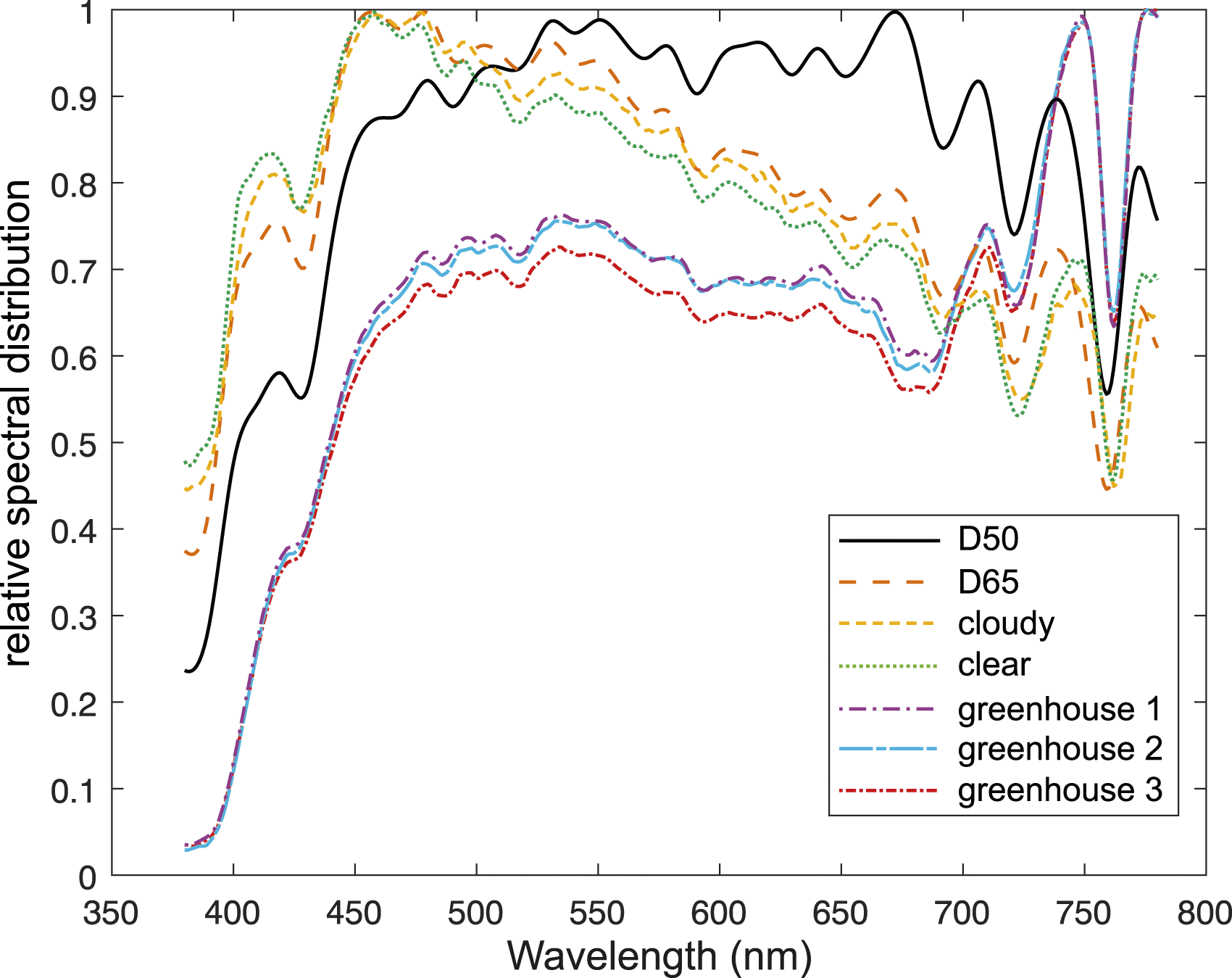
Relative spectral distribution of D50 and D65 daylight spectra, two examples of measured spectra at clear and cloudy sky and three spectral distributions measured under a greenhouse roof

However, using the spectral sensor (sensor 1) with method 1, results are more stable against deviations of the incident spectrum compared to method 2. Due to only 3 channels, the spectral resolution of sensor 2 is not sufficient to measure these deviations. As the spectrum is different from the daylight spectrum, it was expected for method 2 to not lead to useful results.

4. Discussion and future work

Without offset correction, the results in the previous section demonstrate that method 2 based on the CIE-daylight model estimates PPFD best. After appropriate offset correction, all methods are very close to the ideal value, and this has been shown with the test dataset. Additionally, both methods theoretically surpass the accuracy of a commercial quantum sensor under daylight.²⁴ Due to the higher number of sampling points, sensor 1 is closer to the ideal value than sensor 2 using method 1. In addition, method 1 exhibited better stability against unexpected incident spectra.

Due to the calculation of the PPFD based on the CIE daylight model, the second method is not stable against spectral distributions which deviate from the ones used in the training datasets, for example, spectra in greenhouses or daylight mixed with spectra from artificial light sources. For example, the accuracy of the calculation of the PPFD in the case of mixed light from daylight and sodium vapour lamp or LED lamp, as used in modern greenhouses, would decrease significantly when using the second method. Furthermore, the first method is assumed to lose accuracy, but not to the same extent as the second method.

Method 1 can be executed with very little computational effort on a low-cost microcontroller and thus offers the possibility to be integrated into an inexpensive and portable handheld measuring device.^24,25 Leon-Salas et al. ²⁵ measured an error between 1.77 % and 7.3 % for different daylight conditions using the same sensor. Such a dependency on the daylight spectrum was not noticeable in this study, leading to the assumption that this error might not come from the determination of the factor k _e..p.

Without an offset correction, method 2 performs better. For applications where computation power is not a limiting factor, this method could moreover be used to precisely determine the factor k _e..p. Especially useful is this in situations where devices with an already integrated colour sensor, for example, colorimeters, are available to measure PPFD.

All sensors in this work cost approximately 5 USD in small quantities to about 2 USD per chip in large quantities. Ready-to-use development kits for these sensors are in a range between 150 and 200 USD. In contrast, the cost of a handheld spectrometer is about 2500 USD. By calculating PPFD with such a low-cost measurement setup, more people gain access to the technology. Nowadays, most smartphones use built-in ambient sensors for ambient detection and R-G-B camera sensors. It may be possible to calculate the PPFD using those built-in sensors and a smartphone application. In addition, XYZ sensors are becoming more and more common in medical displays (white balance) or colour recognition (LED, skin, hair, printed materials).

For future work, this simulation-based calculation of the PPFD must be transferred into a real measurement setup to evaluate the two methods in a practical application.

For applications in horticulture, the use of method 1 has the possibility to gather information about spectral composition of the light and allows spectral ratios to be adjusted to influence plant physiology. The influence of far red on the plant reveals that the daily dose in this spectral range must be recorded. Simple PAR quantum counters have no sensitivity in this spectral range and thus give no information about these parameters. An extension of the PAR-range to the far-red region in the future, as proposed by Zhen et al,³ could be measured with a spectral sensor. The accuracy in this range should be tested in future experiments.

5. Conclusion

In this work, determination of the conversion factor k _e..p using two approaches was compared. The results demonstrate that both methods are well-suited approach for measurements under daylight. Testing the methods with spectra measured in a greenhouse revealed the benefits of sensor 1, using 8 spectral channels. Depending on the application, this study helps in choosing an appropriate method for measuring PPFD. Theoretically, the sensitivity curves of optical sensors can lead to precise measurements of daylight PPFD. Future work shall focus on real-world measurement with different intensities and compare the conversion factors with the theoretical ones.

Footnotes

Declaration of conflicting interests

The authors declared no potential conflicts of interest with respect to the research, authorship, and/or publication of this article.

Funding

The authors received no financial support for the research, authorship, and/or publication of this article.

ORCID iDs

T Hegemann

J Balasus

QV Trinh

A Herzog

TQ Khanh

References

van Iersel

Chappell

Lea-Cox

. Sensors for improved efficiency of irrigation in greenhouse and nursery production. HortTechnology 2013; 23: 735–746. DOI: 10.21273/HORTTECH.23.6.735.

McCree

. Test of current definitions of photosynthetically active radiation against leaf photosynthesis data. Agricultural Meteorology 1972; 10: 443–453. DOI: 10.1016/0002-1571(72)90045-3.

Zhen

van Iersel

Bugbee

. Why far-red photons should be included in the definition of photosynthetic photons and the measurement of horticultural fixture efficacy. Frontiers in Plant Science 2021; 12: 693445. DOI: 10.3389/fpls.2021.693445.

Albright

Both

Chiu

. Controlling greenhouse light to a consistent daily integral. Transactions of the ASAE 2000; 43: 421–431. DOI: 10.13031/2013.2721.

Pinho

Hytönen

Rantanen

Elomaa

Halonen

. Dynamic control of supplemental lighting intensity in a greenhouse environment. Lighting Research and Technology 2013; 45: 295–304. DOI: 10.1177/1477153512444064.

Schwend

Beck

Prucker

Peisl

Mempel

. Test of a par sensor-based, dynamic regulation of led lighting in greenhouse cultivation of helianthus annuus. European Journal of Horticultural Science 2016; 81: 152–156. DOI: 10.17660/eJHS.2016/81.3.3.

van Iersel

Gianino

. An adaptive control approach for light-emitting diode lights can reduce the energy costs of supplemental lighting in greenhouses. HortScience 2017; 52: 72–77. DOI: 10.21273/HORTSCI11385-16.

Federer

Tanner

. Sensors for measuring light available for photosynthesis. Ecology 1966; 47: 654–657. DOI: 10.2307/1933948.

McCree

. A solarimeter for measuring photosynthetically active radiation. Agricultural Meteorology 1966; 3: 353–366. DOI: 10.1016/0002-1571(66)90017-3.

10.

Biggs

Edison

Eastin

Brown

Maranville

Clegg

. Photosynthesis light sensor and meter. Ecology 1971; 52: 125–131. DOI: 10.2307/1934743.

11.

Booth

. The design and evaluation of a measurement system for photosynthetically active quantum scalar irradiance1. Limnology and Oceanography 1976; 21: 326–336. DOI: 10.4319/lo.1976.21.2.0326.

12.

Muchow

Kerven

. A low cost instrument for measurement of photosynthetically active radiation in field canopies. Agricultural Meteorology 1977; 18: 163–239. DOI: 10.1016/0002-1571(77)90036-x.

13.

Woodward

. Instruments for the measurement of photosynthetically active radiation and red, far-red and blue light. Journal of Applied Ecology 1983; 20: 103–115. DOI: 10.2307/2403379.

14.

Mims

III . A 5-year study of a new kind of photosynthetically active radiation sensor. Photochemistry and Photobiology 2003; 77(1): 30–33. DOI: 10.1562/0031-8655(2003)0770030AYSOAN2.0.CO2.

15.

Caya

MVC

Alcantara

Carlos

Cereno

SSB

. Photosynthetically active radiation (par) sensor using an array of light sensors with the integration of data logging for agricultural application. In: 2018 3rd International Conference on Computer and Communication Systems (ICCCS). Piscataway, NJ: IEEE, 2018: 377–381. DOI: 10.1109/ccoms.2018.8463321.

16.

Yadav

Sumesh

Beno

Karanth

Sadashivappa

. Design of photosynthetically active radiation sensor. Examines in Physical Medicine and Rehabilitation 2018; 1(5). DOI: 10.31031/epmr.2018.01.000521.

17.

Rajendran

Leon-Salas

Fan

Zhang

Vizcardo

Postigo

. On the development of a low-cost photosynthetically active radiation (par) sensor. In: 2020 IEEE International Symposium on Circuits and Systems (ISCAS). Piscataway, NJ: IEEE, 2020: 1–5. DOI: 10.1109/iscas45731.2020.9181220.

18.

McCree

. The measurement of photosynthetically active radiation. Solar Energy 1973; 15: 83–87. DOI: 10.1016/0038-092X(73)90010-8.

19.

Norman

Tanner

Thurtell

. Photosynthetic light sensor for measurements in plant canopies. Agronomy Journal 1969; 61: 840–843. DOI: 10.2134/agronj1969.00021962006100060004x.

20.

Ross

Sulev

. Sources of errors in measurements of PAR. Agricultural and Forest Meteorology 2000; 100: 103–125. DOI: 10.1016/S0168-1923(99)00144-6.

21.

Barnes

Tibbitts

Sager

Deitzer

Bubenheim

Koerner

, et al. Accuracy of quantum sensors measuring yield photon flux and photosynthetic photon flux. HortScience 1993; 28: 1197–1200. DOI: 10.21273/HORTSCI.28.12.1197.

22.

Biosciences LC . Comparison of quantum sensors with different spectral sensitivities. LI-COR Biosciences Technical Note 2018, Retrived from, https://www.licor.com/documents/oi26ib7eb6wm5y5u9ebv4b3jodm09tf9.

23.

Blonquist

Johns

. Accurate PAR measurement: comparison of eight quantum sensor models. Apogee Instruments Research Report 2018, Retrived from, https://www.apogeeinstruments.com/content/Comparison-of-Eight-Quantum-Sensor-Models.pdf (accessed 20 August 2021).

24.

Bäumker

Zimmermann

Schierle

Woias

. A novel approach to obtain PAR with a multi-channel spectral microsensor, suitable for sensor node integration. Sensors 2021; 21: 3390. DOI: 10.3390/s21103390.

25.

Leon-Salas

Rajendran

Vizcardo

Postigo-Malaga

. Measuring photosynthetically active radiation with a multi-channel integrated spectral sensor: 2021 IEEE International Symposium on Circuits and Systems (ISCAS), Daegu, South Korea, May 22–28: 2021; DOI:10.1109/iscas51556.2021.9401321.

26.

AMS . AS7341 11-channel multi-spectral digital sensor. Retrived from, https://ams.com/documents/20143/36005/AS7341_DS000504_3-00.pdf (accessed 20 August 2021).

27.

AMS . TCS3472 color light-to-digital converter with IR filter. Retrived from, https://ams.com/documents/20143/36005/TCS3472_DS000390_3-00.pdf (accessed 20 August 2021).

28.

AMS . AS7264N XYZ chromatic color and 440/490nm blue sensor with electronic shutter. Retrived from, https://ams.com/documents/20143/36005/AS7264N_DS000569_1-00.pdf (accessed 20 August 2021).

29.

Vora

Farrell

Tietz

Brainard

. Digital color cameras - 2 - spectral response. HP Laboratories Technical Report 1997: 97–54.

30.

Hubel

Sherman

Farrell

. A comparison of methods of sensor spectral sensitivity estimation. HP Laboratories Technical Report 1994: 45–48.

31.

CIE . Technical Report 015:2008 Colorimetry. 4th Edition. Vienna: CIE, Central Bureau, 2018. ISBN 978-3-902842-13-8. DOI: 10.25039/TR.015.2018.

32.

McCamy

. Correlated color temperature as an explicit function of chromaticity coordinates. Color Research & Application 1992; 17(2): 142–144. DOI: 10.1002/col.5080170211.

33.

Hegemann

Balasus

Trinh

Herzog

Khanh

. Supplementary data: using spectralsensors to determine Photosynthetic Photon Flux Density (PPFD) in daylight - a theoretical approach. DOI: 10.48328/tudatalib-653. Retrived from, https://tudatalib.ulb.tu-darmstadt.de/handle/tudatalib/2985 2021.

Using spectral sensors to determine photosynthetic photon flux density in daylight – A theoretical approach

Abstract

1. Introduction

2. Experimental details and methods

2.1 Calculating PPFD from spectral irradiance

2.2 Method 1: Determination based on reduced PAR-weighting functions

2.3 Method 2: Determination based on the CIE daylight model

2.4 Determination of the error

3. Results

3.1 Error using method 1

3.2 Error using method 2

3.3 Errors using test spectra dataset

3.4 Errors using greenhouse spectra

4. Discussion and future work

5. Conclusion

Footnotes

Declaration of conflicting interests

Funding

ORCID iDs

References