Unbiased Sampling of Users from (Online) Activity Data

Abstract

Online platforms offer new opportunities to study human behavior. However, while social scientists are often interested in using behavioral trace data—data created by a user over the course of their everyday life—to draw inferences about users, many online platforms only allow data to be sampled based on user activities (leading to data sets that are biased toward highly active users). Here, we introduce a simple method for reweighting activity-based sample statistics in order to provide descriptive (and potentially model-based) estimates of the user population. We illustrate these techniques by applying them to a case study of an online fitness community (Strava) and use it to explore basic network properties. Last, we explore the weights effect on model-based estimates for count data.

Introduction

Probability samples are the gold standard for inference on a population of interest (see, e.g., Kish 1965). This is true for inference of online populations, whether the goal is descriptive analysis, hypothesis testing, or parametric modeling. In general, one needs the ability to enumerate the population of interest and then a mechanism for selecting entities at random. Classically, the preferred method is simple random sampling without replacement (SRS), where each entity is selected with equal probability taking into account that the entity can only be sampled once or simple random sampling with replacement (SRSWR), where each entity is selected with equal probability but can be selected more than once. Applying these techniques to online environments is not always straightforward; we address this challenge here.

Social scientists are often interested in using behavioral trace data—data created by a user over the course of their everyday life—from online platforms to draw inferences about users. However, many online platforms only allow data to be sampled based on user activities or behavior, not users themselves (leading to a data set that is biased toward highly active users). This mismatch arises because the implementation and purpose of many online application programming interfaces (APIs) are to facilitate access to behavioral data. The makers of such applications are focused not on social science research but on extending the usability of the application they have created, making data available to third parties. Take, for example, Strava (http://www.strava.com), the case studied here (Zeng et al. 2017). Strava is a smartphone-based application to track physical activity (e.g., biking, running) and to allow social sharing and interaction between athletes. Data from this platform are made available through its API but can only be accessed through certain points of entry—the potential (and number of) data queries are limited. Thus, one of the major data collection challenges is to construct an appropriate sampling frame for user-based research questions.

Ideally, one would like to be able to draw a random sample of all Strava users and follow their behaviors on the system over time. In practice, this is unfeasible because one cannot uniquely identify all users; moreover, the set of all users is constantly changing as new users join the community. In addition, the Strava API, like many others, does not allow one to query data based on a random user identifier (userID). We can, however, use a rejection sampling strategy on the set of all activities logged by platform users to obtain an approximate SRS. The case of Strava is an exemplar of many online platforms; therefore, the techniques presented in this letter are of broad applicability.

Rejection sampling is a basic technique for generating a sample of observations, in our example case, a set of activity identifiers (activityID) that can be used to collect data from the API. Rejection sampling has been successfully used in the past as a method for generating a truly random sample from online platforms where the set of all possible IDs of interest is enumerable (Gjoka et al. 2010). Under a rejection sampling framework, we consider the set of all theoretically possible activityIDs as our sampling frame and then randomly generate a set of IDs to sample using the Strava API. For each activityID in this set, we execute the query to see whether that activityID exists on the platform. In cases where an activity is found (i.e., that activityID exists), we sample it and collect data. In cases where the activity does not exist, we reject the generated ID from the sample.

Given a particular (existing) activityID, it is then possible to utilize the Strava API to collect various data related to the activity itself (e.g., location, duration). As each activityID is associated with a particular user, one can also access additional user-level data. This includes user features as well as social ties. In this way, the activityID serves as an entry point or access point through which other data, in particular user-based features, can be collected.

Many problems of interest are centered on users (e.g., preferential attachment, diffusion) and not activities (e.g., a single instance of running). Other online platforms with this same structure include runkeeper, myfitnesspal, pinterest, and so forth. Moreover, there are new online environments coming online everyday. Here, we propose a straightforward method for building sample weights under this basic sampling strategy so as to allow for unbiased estimation of descriptive statistics and for use in parametric inference (e.g., linear models) for the user population based on activity sampling.

We begin by laying out the sampling theory we build our estimates on. We then derive a set of sampling weights based on combinatorics of the finite population and use these estimates to derive large sample weights; next, we apply these methods to a large sample of Strava data as a case study; then, we follow up with some sensitivity tests via simulation, and finally, we conclude with a few remarks.

Sample Theory

In sampling theory, the Horvitz–Thompson (HT) estimator is a statistical technique for estimating the total and mean of a population when sampling without replacement (Horvitz and Thompson 1952). The Hansen–Hurwitz estimator is a method for estimating the total and mean of a population for sampling with replacement (Hansen and Hurwitz 1943). We only discuss the HT estimator here, but the procedure is analogous for SRSWR. Inverse probability weighting is applied to account for different proportions of observations within strata or clusters in a target population. The HT estimator is often applied in survey analyses setting and can be used to account for missing data. 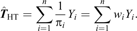Formally, let Y_i, $i = 1, 2, \dots, n$ be an independent sample from n of $N \geq n$ with a mean μ, where n is the sample size. Suppose further that π_i is the inclusion probability that a randomly sampled individual in a population belongs to the i th stratum. The HT estimate of the total is given by:

{\hat{T}}_{HT} = \sum_{i = 1}^{n} \frac{1}{π_{i}} Y_{i} = \sum_{i = 1}^{n} w_{i} Y_{i} .

The HT estimate of the mean is given by:

{\hat{μ}}_{HT} = \frac{1}{N} \sum_{i = 1}^{n} \frac{1}{π_{i}} Y_{i} = \frac{1}{N} \sum_{i = 1}^{n} w_{i} Y_{i} .

Thus, all that is required to obtain the total and mean for a population is population size (N) and the inclusion probability π_i for all outcomes (Y_i) sampled. These resulting weights, w_i, can further be used within parametric models (e.g., linear models) for improved inference (Pfeffermann 1993).

Deriving Weights for User-based Samples

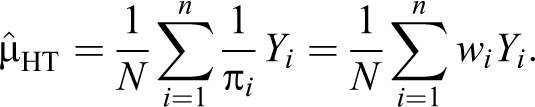
Our setup is the following: We have a universe ( $U$ ) of activities ( $a_{i} \in A$ ) with associated users ( $u_{k} \in U$ ), where each a_i is unique, but no such requirement is made for the users as users can be associated with more than one activity that they have posted. So, we have $U = {{a_{1}, u_{(1)}}, \dots, {a_{N_{a}}, u_{(N_{u})}}$ , where $| A | = N_{a}$ , $| U | = N_{u}$ , and $(\cdot) = (1), \dots, (n)$ denotes nonunique occurrence. If we take a simple random sample (SRS) of size n of A, then the inclusion probability is $Pr (a_{i}) = \frac{n}{N_{a}}$ ; however, the probability of sampling a given user (the item of interest) is not so simple. First, let us define $D_{i} = {# of activities$ u_i $participates in}$ , then probability of sampling a given user is,

\begin{array}{l} Pr (u_{i}) = \sum_{i = 1}^{D_{i}} Pr (a_{i}) - \sum_{i_{1} < i_{2}} Pr (a_{i_{1}} \cap a_{i_{2}}) + \sum_{i_{1} < i_{2} < i_{3}} Pr (a_{i_{1}} \cap a_{i_{2}} \cap a_{i_{3}}) \\ - \dots + {(- 1)}^{D_{i} + 1} Pr (a_{1} \cap a_{2} \dots \cap a_{D_{i}}), \\ = D_{i} \frac{n}{N_{a}} - (\begin{matrix} D_{i} \\ 2 \end{matrix}) \frac{(\begin{matrix} N_{a} - 2 \\ n - 2 \end{matrix})}{(\begin{matrix} N_{a} \\ n \end{matrix})} + (\begin{matrix} D_{i} \\ 3 \end{matrix}) \frac{(\begin{matrix} N_{a} - 3 \\ n - 3 \end{matrix})}{(\begin{matrix} N_{a} \\ n \end{matrix})} \\ + \dots + {(- 1)}^{D_{i} + 1} \frac{(\begin{matrix} N_{a} - D_{i} \\ n - D_{i} \end{matrix})}{(\begin{matrix} N_{a} \\ n \end{matrix})} . \end{array}

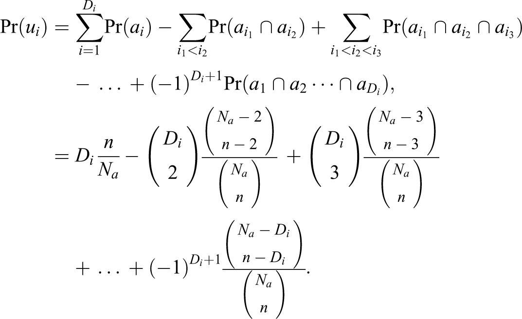
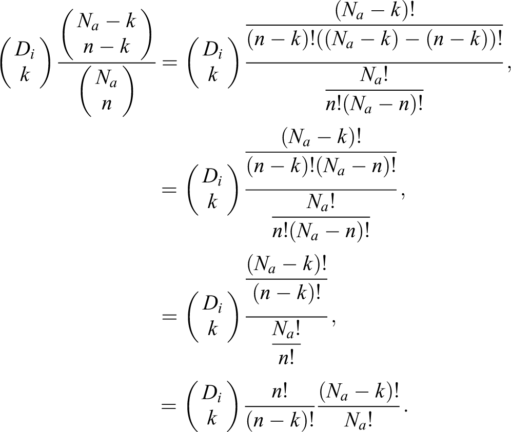
Let us pick the kth term for $1 < k \leq D_{i}$ in this expression and solve it,

\begin{matrix} (\begin{matrix} D_{i} \\ k \end{matrix}) \frac{(\begin{matrix} N_{a} - k \\ n - k \end{matrix})}{(\begin{matrix} N_{a} \\ n \end{matrix})} = (\begin{matrix} D_{i} \\ k \end{matrix}) \frac{\frac{(N_{a} - k)!}{(n - k)! ((N_{a} - k) - (n - k))!}}{\frac{N_{a}!}{n! (N_{a} - n)!}}, \\ = (\begin{matrix} D_{i} \\ k \end{matrix}) \frac{\frac{(N_{a} - k)!}{(n - k)! (N_{a} - n)!}}{\frac{N_{a}!}{n! (N_{a} - n)!}}, \\ = (\begin{matrix} D_{i} \\ k \end{matrix}) \frac{\frac{(N_{a} - k)!}{(n - k)!}}{\frac{N_{a}!}{n!}}, \\ = (\begin{matrix} D_{i} \\ k \end{matrix}) \frac{n!}{(n - k)!} \frac{(N_{a} - k)!}{N_{a}!} . \end{matrix}

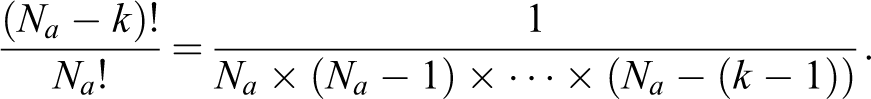
Notice that $(\begin{matrix} D_{i} \\ k \end{matrix}) \frac{n!}{(n - k)!}$ is finite and only depends on the sampling decisions. If we then look at $\frac{(N_{a} - k)!}{N_{a}!}$ , we can simplify this to

\frac{(N_{a} - k)!}{N_{a}!} = \frac{1}{N_{a} \times (N_{a} - 1) \times \dots \times (N_{a} - (k - 1))} .

Therefore,

lim_{N_{a} \to \infty} \frac{(N_{a} - k)!}{N_{a}!} = 0.

This holds for all $k = 2, \dots, D_{i}$ ; therefore, we can approximate $Pr (u_{i})$ by,

Pr (u_{i}) \approx D_{i} \frac{n}{N_{a}} when N_{a} is approximately large .

We find that in practice $Pr (u_{i})$ (π_i in our example) can be approximated best by this limiting case in most applied settings; we demonstrate this finding in Sensitivity Test via Simulation section through careful simulation analysis. In practice, D_i and N_a are not usually known, so they will also have to be estimated via the HT estimator. In the next section, we discuss a natural strategy for such an issue.

Estimating D_i and N_a

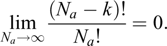
In the above derivation, we “tacitly” assumed that D_i and N_a are known; however, this is typically not true for sampling behaviors in online contexts. There are many possible ways to estimate these parameters, including using the acceptance rate in the rejection sampling context. But, we suggest starting with following procedure: In many online contexts, users are required to have a public profile (could be just their user ID), which is typically attached to a given numeric ID. If the space for the numeric ID is fixed, say K digits and mostly filled up, we can again use rejection sampling to estimate the size of the user population. Further, if we assume the numeric IDs are assigned sequentially, we can use the largest digit with a user ID as the total number of users. We are usually interested in the active user population (i.e., users who did more than just sign up for the app) and not just the “user” population. We define $N_{u}^{active}$ as the number of active users in the population over a given time point (t), for example, users who have engaged the app in the last year. Given a sample S of activities and associated users, one can estimate $N_{u}^{active}$ by taking a random sample of the user ID space and considering the last date that user was active and specify what our time window is (say, however long we have been sampling), that is,

{\hat{N}}_{u}^{active} = N_{u}^{Max} \times \frac{# of active users in the time frame}{Size of the random sample of the User ID Space} .

Let $A_{i} : = {# activities of user i in S}$ , then we can estimate,

{\hat{D}}_{i}^{active} = {\hat{N}}_{u}^{active} \times \frac{A_{i}}{| S |} .

Empirical Case: Gender-based Network Characteristics on Strava

We developed and then employed the sampling scheme described in the Introduction section to obtain an SRS of 888,093 activities on the activity tracking platform Strava. As described previously, Strava data are available through its API, but access points provide biased samples when the researcher’s goal is individual-level (i.e., user) inference. The data collected in this pilot study, for example, posted activities, span the period from 2011 until 2016. Recall, the activity sampling procedure is one of rejection sampling; here, the sample had an average acceptance rate of 90.274%, from which we infer that the activity space we considered was quite filled. Our goal in this preliminary study was to look at personal network characteristics (e.g., size), as well as the gendered nature of interpersonal ties in this environment. Strava is unique in that the platform is heavily male dominated, motivating our exploration of whether or not formed relationships were gendered. To address these questions, we employ the approach outlined in the Deriving Weights for User-based Samples section.

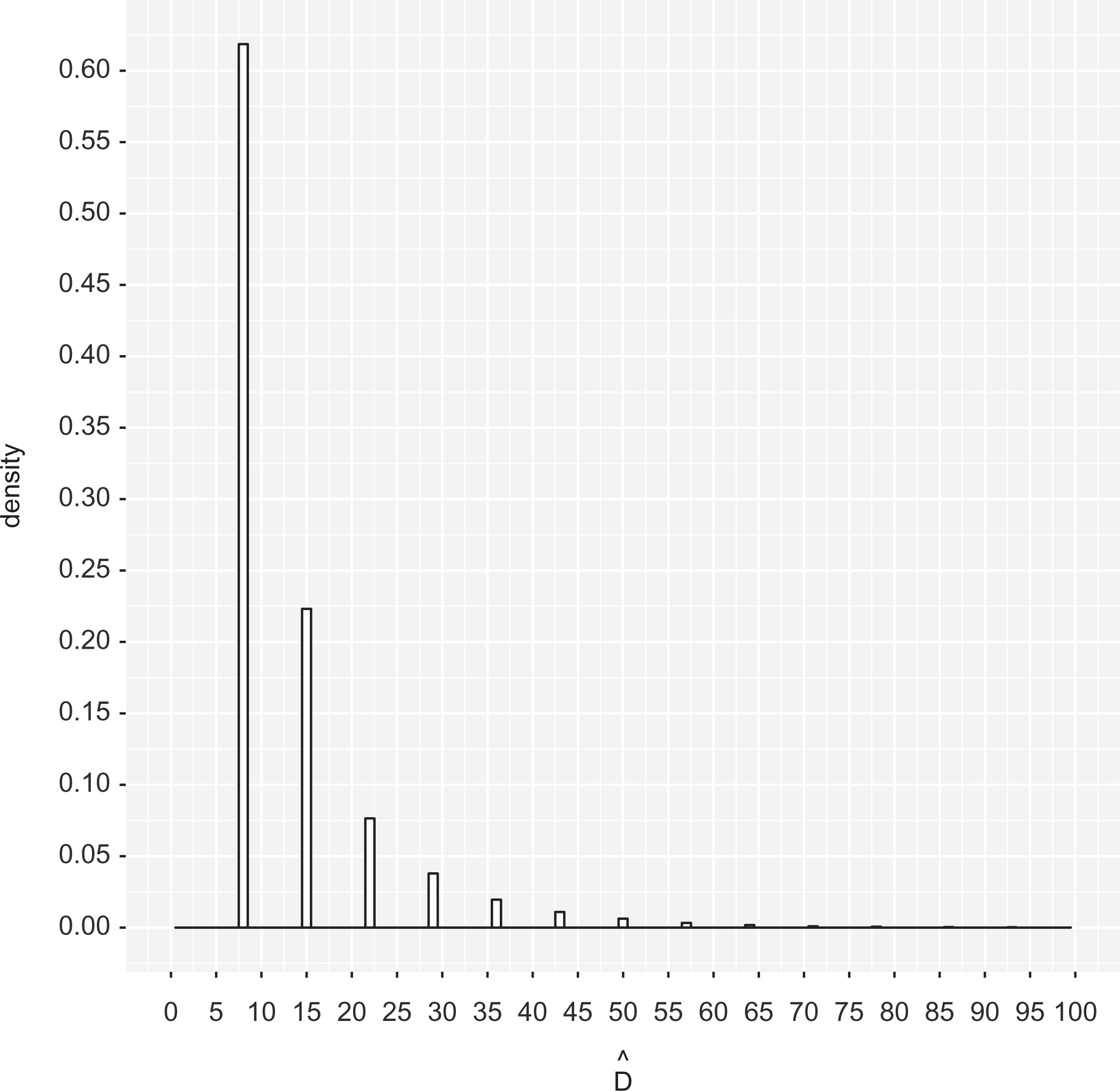
First, following the procedures for the Estimating D_i and N_a subsection, we obtained estimates for $\hat{D}$ and ${\hat{N}}_{a}$ by observing that the largest activityID on the last day of data collection was 18,676,848 and employing HT estimator to estimate the active population. The density of the userID space was obtained from a proportion estimator of an SRS¹ on the userID space ( ${\hat{p}}_{userIDSpace} = .98$ ), and the active user population data were obtained from the same SRS checking to see whether the user was active in the last year ( ${\hat{p}}_{active} = .344$ ). These estimates are subsequently used to estimate the following key quantities, ${\hat{N}}_{u} = 18, 303, 311$ , ${\hat{N}}_{a} = 1, 986, 028, 000$ , and $\hat{D}$ . The estimated distribution of activities per user, $\hat{D}$ , is seen in Figure 1.

Figure 1.

Estimated distribution of activities per Strava user. The graph is zoomed in to show the concentration of activities. There is a long tail of 160 data points above the 150 threshold.

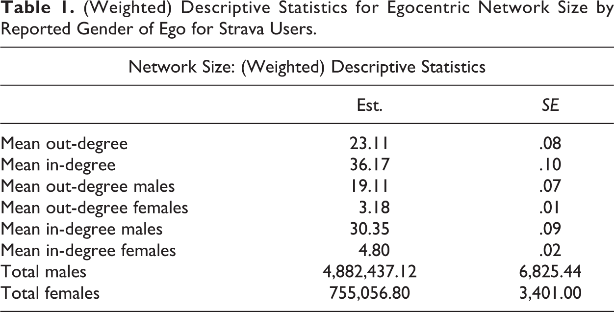
We use the derived inclusion probabilities from the Deriving Weights for User-based Samples section to estimate the mean degree (number of social contacts) of individuals in the Strava sample. Once a researcher has the above weights, he or she can use classic sampling software (here, we use Lumley [2004] survey package in R Version 3.4.1) for mean/total estimation and variance² estimation. We apply these methods to describe the average degree statistics for personal networks on Strava (see Table 1). We further compare gender-based assortative mixing properties of the network (see Table 2).

Table 1.

(Weighted) Descriptive Statistics for Egocentric Network Size by Reported Gender of Ego for Strava Users.

Network Size: (Weighted) Descriptive Statistics
	Est.	SE
Mean out-degree	23.11	.08
Mean in-degree	36.17	.10
Mean out-degree males	19.11	.07
Mean out-degree females	3.18	.01
Mean in-degree males	30.35	.09
Mean in-degree females	4.80	.02
Total males	4,882,437.12	6,825.44
Total females	755,056.80	3,401.00

Table 2.

(Weighted) Descriptive Statistics for Gender-based Assortative Mixing among Strava Users.

Assortative Mixing: (Weighted) Descriptive Statistics
	Est. Num. Ties	SE
Male friends	24.67	.09
Female friends	15.73	.17
Male to male friends	20.85	.08
Male to female friends	10.18	.12
Female to female friends	4.97	.06
Female to male friends	2.96	.02

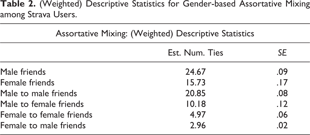
As Tables 1 and 2 demonstrate, males have larger personal networks, with higher counts of both incoming and outgoing ties. We also see evidence for high level of gender-based homophily, which is particularly strong for males.

Small Sample Analysis of Estimated Weights

To understand the relationship between our estimated weights and the exact weights, we perform a sensitivity analysis of the small sample properties of our estimator against the exact weights. In Table 3, we do a sensitivity analysis, where we assume different sizes of the universe of activities ( ${\hat{N}}_{a}$ ) and different sample sizes (n) obtained by drawing a random sample from that universe. Then, for each of the ${\hat{N}}_{a}$ and n combinations where $n < {\hat{N}}_{a}$ , we compute the exact and approximate inclusion probabilities $(π_{i}^{exact}$ and $π_{i}^{approx}$ ). Then, we invert these inclusion probabilities to get the weights w_i ( $w_{i}^{Exact}$ and $w_{i}^{Approx}$ , respectively) as in the HT estimate. Table 3 corresponds to the mean difference of those weights, averaged over all users in the sample, that is,

= \frac{1}{n} \sum_{i = 1}^{n} (w_{i}^{approx} - w_{i}^{exact}) where w_{i}^{approx} = \frac{1}{π_{i}^{approx}} and w_{i}^{exact} = \frac{1}{π_{i}^{exact}} .

Table 3.

Absolute Mean Difference between Approximate and Exact Weights for Different Population ( ${\hat{N}}_{a}$ ) and Sample Size (n) Combinations.

	${\hat{N}}_{a}$ (Number of Activities)
*n (sample size)	10²	10³	10⁴	10⁵	$5 \times 10^{5}$
10	6.095581	1.349713	≈0	≈0	≈0
10²		6.11987	1.368719	≈0	≈0
10³			6.122267	1.367879	2.410588 × 10⁻¹¹
10⁴				6.122506	10.74351
10⁵					2.629058

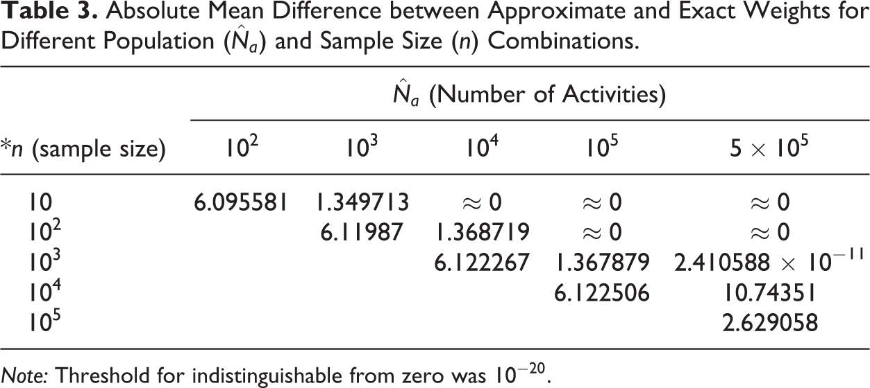
Note: Threshold for indistinguishable from zero was $10^{- 20}$ .

It can be seen from the table that as the population size increases and the sample size drawn is reasonably small (approximately less than 0.001 times the population size) as compared to the population, then the difference in two weight estimates is infinitesimally small. For our Strava data, we have ${\hat{N}}_{a} \approx 2 \times 10^{9}$ and the sample is about $n \approx 8 \times 10^{5}$ . Hence, the population size is large and the sample size is reasonably small, so we also see that the exact and approximate weights are very similar. Therefore, in our analysis, we just show results using the approximate weights. We don’t see very good results for the other cases (when N_a is small and n is not considerably small as compared to ${\hat{N}}_{a}$ ) in terms of the difference in the exact and approximate estimates being similar. This could be attributed to the limitation of the combinatoric approximation we make where the condition $| 2 n - k | = o (n^{3 / 4})$ may have been violated. However, we observe that the large weight corresponds to relatively small change in the inclusion probability (e.g., $π^{approx} \approx 0.03$ with corresponding $π^{exact} \approx 0.04$ ) and thus may not be as worrisome as the table makes it appear.

Sensitivity Test via Simulation

To see the importance of the weights derived in the Deriving Weights for User-based Samples section, we run simulations on subsamples of the original data set and compare the weighted and unweighted results for these subsamples. The procedure for the simulations is as follows: first, obtain subsamples starting from 1% of the data to 100% of the data, then calculate both the weighted (using limiting weights) and unweighted average degree statistics for personal networks formed by these subsamples. Next, obtain 95% bootstrap standard errors for these estimates by repeatedly resampling (with replacement) from that subsample, calculating the sample mean estimates for each of the samples obtained as a result of resampling and then calculating the standard deviation of these estimates. After this, we also find empirical distribution by repeated subsampling from the original data and obtaining estimates for mean and standard error. These results for out- and in-degree statistics reported by gender can be found in Tables 5 and 6 of the Online Appendix.

From the results, we can see that as the size of the subsample increases, the difference in the weighted and unweighted estimates increases. While the weighted mean estimates do not change much with sample size, the unweighted mean estimates decrease as the sample size increases. Empirical standard errors seem to be smaller than bootstrap standard errors which, in turn, seem to be smaller than the subsample standard errors.

We also calculate the nonapproximate weights as discussed in the Deriving Weights for User-based Samples section. To calculate these weights, we use binomial approximation for the binomial coefficients in Stanica (2001) and we notice that the difference between the inclusion probabilities calculated using the nonapproximate formula is extremely close to those calculated using the approximate(limiting) formula for all the subsamples. 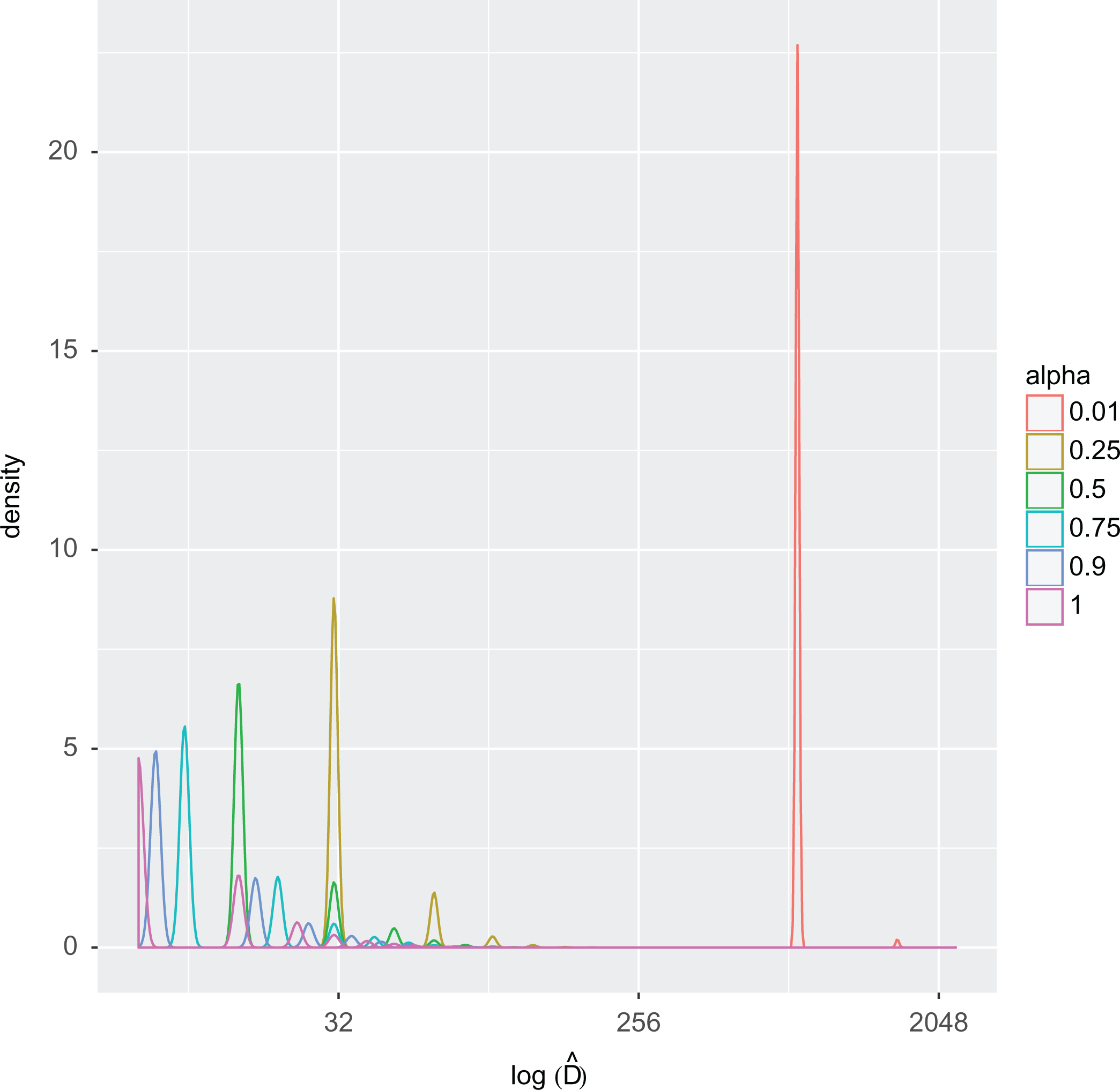For example, for the 25% subsample, the mean difference between approximate and nonapproximate inclusion probabilities is of the order $10^{- 19}$ . Further, the estimated distribution of activities per user $\hat{D}$ for various subsamples is seen in Figure 2.

Figure 2.

Estimated distribution of activities per Strava user for different subsamples, where α denotes the proportion of data points for that particular subsample.

Degree Distribution Comparisons

We would want to compare the degree distribution of weighted and unweighted case for different subsamples, namely, 1%, 10%, 50%, and 100% of the data. The way the comparison works is that we compute the total estimate (using the HT estimator) or the count of Kth degree individuals for both weighted and unweighted case.

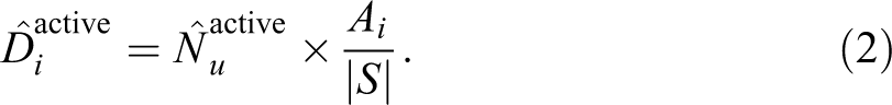
We take a sample of the data that has n_u number of users and n number of activities. Now to compare the total number HT estimates for each degree in the weighted and unweighted case, we have the following: for degree = 1,

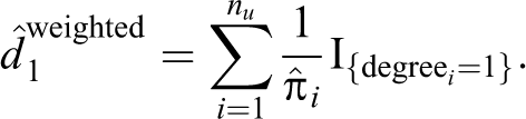
{\hat{d}}_{1}^{weighted} = \sum_{i = 1}^{n_{u}} \frac{1}{{\hat{π}}_{i}} I_{{{degree}_{i} = 1}} .

Substituting ${\hat{π}}_{i}$ from equation 1,

= \sum_{i = 1}^{n_{u}} \frac{{\hat{N}}_{a}}{{\hat{D}}_{i}^{active} n} I_{{{degree}_{i} = 1}},

= \sum_{i = 1}^{n_{u}} \frac{{\hat{N}}_{a} \times | S |}{{\hat{N}}_{u}^{active} \times A_{i} \times n} I_{{{degree}_{i} = 1}} .

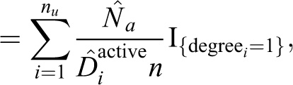
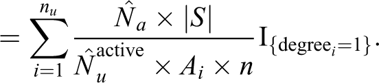
From equation 2,

Then, weighted estimate is given by:

{\hat{d}}_{1}^{Unweighted} = \sum_{i = 1}^{n_{u}} \frac{{\hat{N}}_{u}^{active}}{n} I_{{{degree}_{i} = 1}} .

Likewise, we could find estimates for other degrees. In general, the estimates will be given by:

Weighted estimate: For degree K ≥ 1,

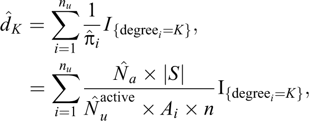
\begin{matrix} {\hat{d}}_{K} = \sum_{i = 1}^{n_{u}} \frac{1}{{\hat{π}}_{i}} I_{{{degree}_{i} = K}}, \\ = \sum_{i = 1}^{n_{u}} \frac{{\hat{N}}_{a} \times | S |}{{\hat{N}}_{u}^{active} \times A_{i} \times n} I_{{{degree}_{i} = K}}, \end{matrix}

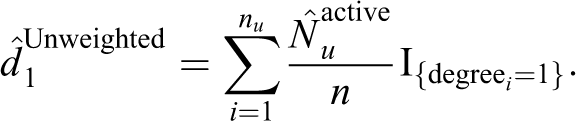
where ${\hat{π}}_{i}$ is the estimated inclusion probability for ith individual, and n is the size of the sample.

Unweighted estimate: For degree K ≥ 1,

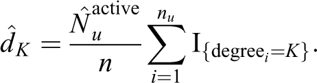
{\hat{d}}_{K} = \frac{{\hat{N}}_{u}^{active}}{n} \sum_{i = 1}^{n_{u}} I_{{{degree}_{i} = K}} .

Figure 3 shows these total number estimates for the various values of degree(K) that occur in the subsample (we consider 1%, 10%, 50%, and 100% of the total data size). As the estimates are skewed toward lower degree, for clarity, we display them on a log scale. Along with that, the shaded regions in green and red give 95% normal bootstrap confidence intervals for these estimates.

Figure 3.

Total number estimates for the various values of degree (K) that occur in a subsample of the Strava data; here, we consider 1%, 10%, 50%, and 100% of the total data size.

Model Fitting for Comparisons

Now, we want to model the degrees of individuals as a function of the weights and other covariates such as gender, membership status (premium or not), and number of activities performed by the individual. The gender level of females is set to be the baseline level with “other” gender and males as the other two categories. The main goal is to compare models with and without the weights and see which one performs better. Since the number of cases with zero degree is too large in comparison to other degree cases, we use zero-inflated generalized linear models (GLMs). GLMs are used because we have count variable as the response (degree of individuals).

Different models are fit, namely, simple Poisson model with weights, zero-inflated Poisson model with and without weights, negative binomial model with weights, and zero-inflated negative binomial model with and without weights. We compare these models using Vuong’s nonnested test that compares two model that do not nest and fit to the same data. It is a likelihood-ratio-based test for model selection using the Kullback–Leibler information criterion. The statistic tests the null hypothesis that the two models are equally close to the true data generating process, against the alternative that one model is closer.

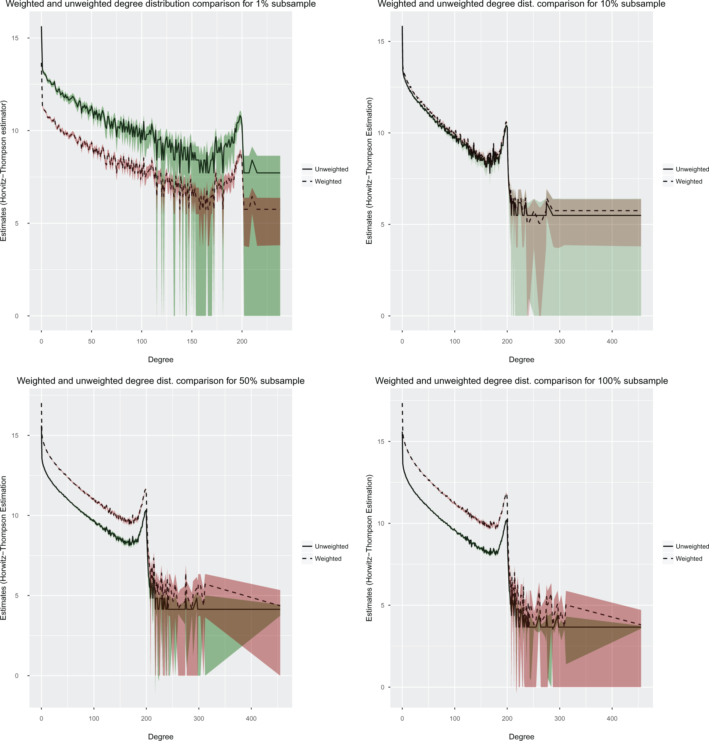
Based on the comparisons made using Vuong’s nonnested tests, we see that the zero-inflated negative binomial model with weights (marked as red in the table) performs the best. The results including the coefficients for different models are given in Table 4. All the variables are significant at a significance level of .05, with a very low p value ( ${< 10}^{- 6}$ ) in all the models.

Table 4.

Different Models Fitting Degree of Individuals as a Function of Some Covariates, with and without the Weights.

	(Intercept)	Gender Other	Gender Male	Premium Membership	Weight	$\hat{D}$
Zero-inflated Poisson (weights)	3.3949	−.4062	.2582	.4932	−.0016	.0022
Poisson (weights)	2.8439	−.3164	.4159	.3760	−.0014	.0018
Negative binomial (weights)	2.8301	−.2984	.4373	.3912	−.0014	.0021
Zero-inflated negative binomial (weights)*	3.2437	−.4152	.3187	.5426	−.0018	.0029
Zero-inflated Poisson (no weights)	2.9914	−.4104	.2692	.5323		.0061
Zero-inflated negative binomial (no weights)	2.6894	−.4185	.3194	.5504		.0160

*Zero-inflated negative binomial with weights performs the best.

Discussion

In this article, we have outlined a simple strategy for sampling (activities/behaviors) to obtain a random sample of individuals (e.g., Strava users). First, we have derived a simple procedure for reweighting the activity data to produce our random sample with good properties. Second, we have introduced simple estimators for commonly unknown fixed quantities required to use the sample weights; then, we employed these weights in a real-world case to get unbiased estimates of the mean degree of Strava users by gender and their resulting standard errors. Last, we employed simulation analysis to test the sensitivity of the weights and the approximation procedure—where we found that the weights become increasingly important as the sample size increases and that the approximation procedure is quite robust. While a complete discussion of this case study, and its results, is outside the scope of this article, these results will likely have implications for group social dynamics and peer influence in activity-based online communities in general. Even this simple, descriptive analysis illustrates the value of developing methods for utilizing activity-based samples for user inference.

Supplemental Material

OnlineAppendix - Unbiased Sampling of Users from (Online) Activity Data

OnlineAppendix for Unbiased Sampling of Users from (Online) Activity Data by Zack W. Almquist, Sakshi Arya, Li Zeng, and Emma Spiro in Field Methods

Footnotes

Declaration of Conflicting Interests

The author(s) declared no potential conflicts of interest with respect to the research, authorship, and/or publication of this article.

Funding

The author(s) disclosed receipt of the following financial support for the research, authorship, and/or publication of this article: This material is based upon work supported by, or in part by, the US Army Research Laboratory and the US Army Research Office under YIP awards #W911NF-14-1-0577 and #W911NF-15-1-0270 and the Office of the Vice President for Research, University of Minnesota.

Supplemental Material

Supplemental material for this article is available online.

Notes

References

Gjoka

Kurant

Butts

C. T.

Markopoulou

. 2010. Walking in Facebook: A case study of unbiased sampling of OSNs. In Infocom, 2010 Proceedings IEEE, pp. 1–9.

Hansen

M. H.

Hurwitz

W. N.

. 1943. On the theory of sampling from finite populations. The Annals of Mathematical Statistics 14:333–62.

Horvitz

D. G.

Thompson

D. J.

. 1952. A generalization of sampling without replacement from a finite universe. Journal of the American Statistical Association 47:663–85.

Kish

1965. Survey sampling. New York: John Wiley & Sons.

Lumley

(2004). Analysis of complex survey samples. Journal of Statistical Software 9:1–19.

Pfeffermann

1993. The role of sampling weights when modeling survey data. International Statistical Review/Revue Internationale de Statistique 61:317–37.

Stanica

2001. Good lower and upper bounds on binomial coefficients. Journal of Inequalities in Pure and Applied Mathematics 2:30.

Zeng

Amquist

Z. W.

Spiro

E. S.

2017. Let’s workout! Exploring social exercise in an online fitness community. In iConference 2017 Proceedings, Vol. 2, pp. 87–98.

Supplementary Material

Please find the following supplemental material available below.

For Open Access articles published under a Creative Commons License, all supplemental material carries the same license as the article it is associated with.

For non-Open Access articles published, all supplemental material carries a non-exclusive license, and permission requests for re-use of supplemental material or any part of supplemental material shall be sent directly to the copyright owner as specified in the copyright notice associated with the article.

0.00 MB

0.10 MB

Unbiased Sampling of Users from (Online) Activity Data

Abstract

Introduction

Sample Theory

Deriving Weights for User-based Samples

Estimating Di and Na

Empirical Case: Gender-based Network Characteristics on Strava

Small Sample Analysis of Estimated Weights

Sensitivity Test via Simulation

Degree Distribution Comparisons

Model Fitting for Comparisons

Discussion

Supplemental Material

OnlineAppendix - Unbiased Sampling of Users from (Online) Activity Data

Footnotes

Declaration of Conflicting Interests

Funding

Supplemental Material

Notes

References

Supplementary Material

Estimating D_i and N_a