Using the Census Planning Database to Generate Differential Expected Yield Rates to Self-administered Mail Surveys

Background

In combination with other inputs such as target completes, precision goals, and budgetary constraints, the expected yield rate in a self-administered mail survey is used to determine the initial sample size. The yield rate is defined as the number of completes ultimately obtained divided by the initial sample size. It is a single quantity simultaneously accounting for undeliverable mailings, household ineligibility (if applicable), and unit nonresponse. Given the expected yield rate and target number of completes, one simply multiplies the target number of completes by the inverse of the yield rate to arrive at the starting sample size needed.

Repeated mail surveys have the luxury of using historical yield rates for planning purposes. Establishing expected yield rates for a new mail survey effort generally requires locating a comparable survey to serve as a reference, and this is naturally an imperfect endeavor since factors such as topic, sponsor, incentive amount, and other subtle features of the data collection protocol can have an impact (Dillman et al. 2014; Groves and Peytcheva 2008). Another complexity is that the expected yield rates may not only be needed overall, but also for specific geographies within the broader study area. For example, the 2020 Healthy Chicago Survey (HCS) aimed for 4,500 completes citywide, but also targeted 35 completes within each of 77 mutually exclusive community areas (i.e., sampling strata). Provided an overall expected yield rate for a mail survey, this short take describes a simple method for merging information from the publicly available tract-level Census Planning Database (PDB) to ascribe differential yield rates to particular geographies that may help inform respective over- or under-sampling needs.

As described in Akers and Alnwick (2001), the first iteration of the PDB was as a resource for the 2000 Decennial Census—in particular, for identifying areas where enumerators might experience barriers or where special procedures need be applied. It consisted of a range of housing, demographic, and socioeconomic variables from the 1990 Decennial Census. Its latest version (accessible via https://www.census.gov/topics/research/guidance/planning-databases.html) contains hundreds of variables that can be used for a myriad of purposes. Some of these variables are derived from the most recent Decennial Census, and others from the American Community Survey (ACS) five-year data file. Pertinent to this short take is the ACS self-response rate variable capturing the rate at which eligible housing units responded during the first phase of ACS data collection, one that involves a sequential series of mail contacts to complete the ACS by web, paper, or telephone questionnaire assistance. Note that the self-response rate excludes from the numerator responses obtained during the subsequent phases of outbound telephone and in-person data collection modes.

Procedure

Application

We have found this technique to produce promising results in recent self-administered mail surveys. For example, it was used in planning for the 2020 HCS, which had newly transitioned from an interviewer-administered random-digit dialing telephone survey to a self-administered format. Specifically, the 2020 HCS was the first in the series to offer web and paper data collection modes to an address-based sample (Harter et al. 2016) of households stratified into community areas, geographies defined by aggregations of census block groups. Note that, since census block groups are nested within census tracts, the same value of P _i was used for all addresses within a census block group.

Figure 1 is a scatterplot of the PDB-derived expected yield rates (2019 vintage) versus the yield rates ultimately observed for the 77 community areas of interest. The plot is overlaid with a 45-degree reference line and a simple linear regression line. While there is some evidence that observed yield rates tend to surpass expectations in lower yield areas and fall short of expectations in higher yield areas, we were encouraged to find the correlation between the two rates to be ρ = 0.74. Note that the 14,799 sampled addresses for the HCS survey were released at two separate points in time during the summer and fall of 2020. Yield rates observed in the first release supplanted the PBD-derived yield rates when planning for the second release. Interestingly, the correlation between rates observed during the first and second releases was lower (ρ = 0.52), but this could be attributable to more noise in the second releases’ rates. The number of sampled addresses in the first release was roughly four times the number in the second release. Plans for the 2021 HCS are to maintain two releases, but with an equal number of sampled addresses in each. Of particular interest will be to determine which yield rates track closer with those to be observed in the 2021 HCS, the 2020 HCS rates or the latest version of PBD-derived rates.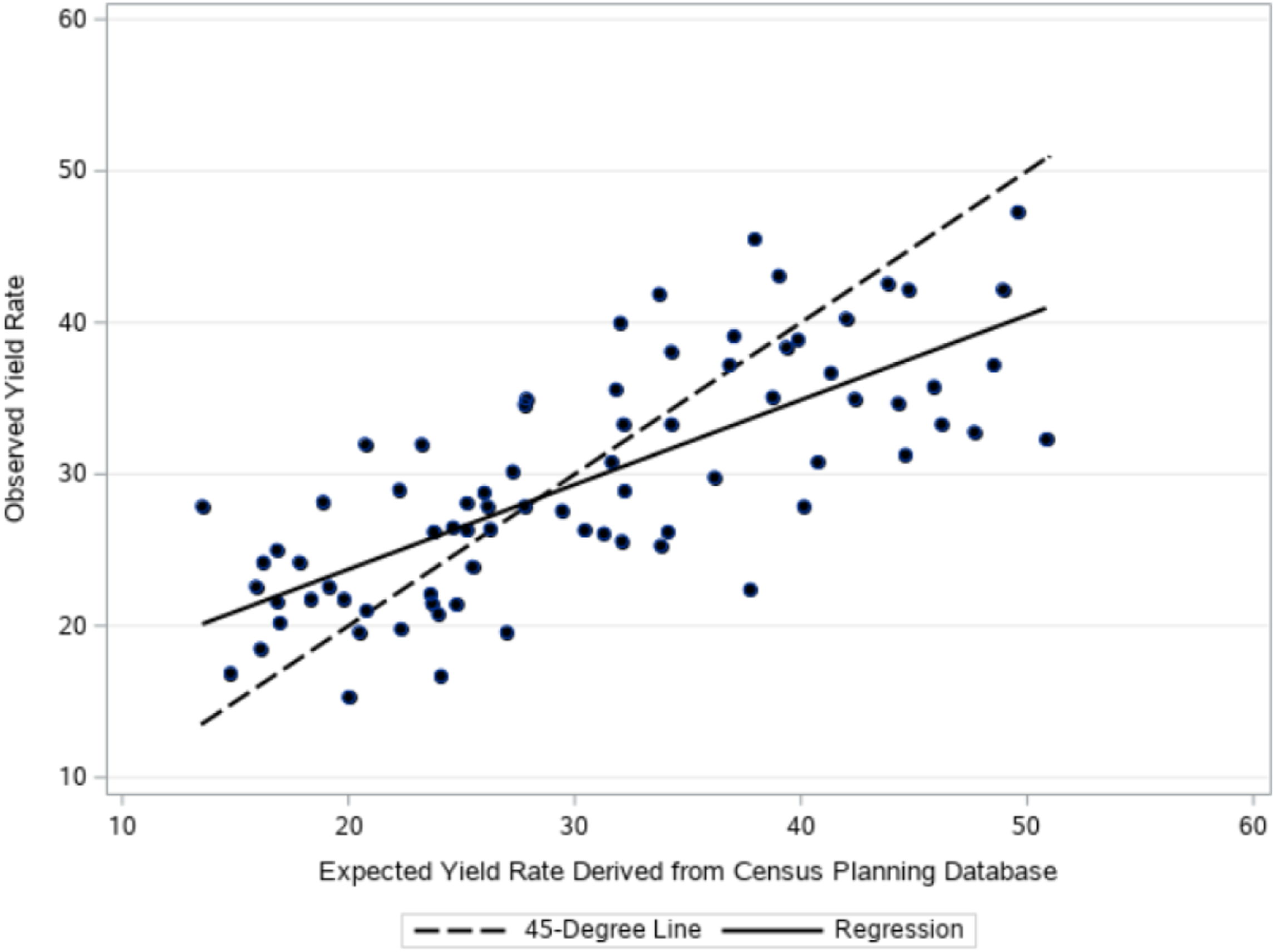OPEN IN VIEWER

Lessons Learned and Limitations

One lesson learned in applying this technique is that the differential expected yield rates calculated may lead to requisite sample sizes that conflict with other constraints, such as the overall sample size accommodated by the survey’s budget or the tolerable precision loss attributable to variable selection probabilities (Kish 1992). This can lead to a breakdown in how the total sample size for the survey is allocated. Potential workarounds include truncating the distribution of expected yield rates, modifying the value input for EYR, or modifying the overall target number of completes. Indeed, some truncation of expected yield rates across community areas was required in the 2020 HCS application, but this did not substantively impact our ability to meet CA-specific target completes or the magnitude of the correlation coefficient with observed yield rates.

Two limitations to the approach are worth noting. The first is that it can only be used for locatable addresses. The Census Bureau’s tract code lookup tool will not work for addresses identified by PO boxes or rural routes, for example. A second limitation is that, until more research is conducted to prove otherwise, we recommend using the approach only for surveys conducted in a self-administered mode via mail contact. A study by Zhu and colleagues (2018) evaluating the predictive ability of PDB-derived performance measures analogous to ours did not produce promising results. Their technique was applied retrospectively for two in-person surveys, however, and used a different metric, the Low Response Score (Erdman and Bates 2017) derived from the 2010 Decennial Census. Similarly, Murphy et al. (2017) conducted an experiment during the 2015 Residential Energy Consumption Survey, finding the correlation of the Low Response Score was in the direction expected for a portion of sample assigned to complete the survey by mail, but not for the complementary portion designated for in-person data collection. Even within the confines of a mail contact, self-administered mode, additional research evaluating our approach would be insightful, particularly for other survey topics (e.g., political attitudes and general market research), surveys covering different or larger areas of the United States, or surveys sponsored by other, non-government entities (e.g., academic, commercial, or nonprofit institutions).