
Abstract
This article assesses the relative efficiency of teams participating in Formula One (F1) World Constructors’ Championship. A nonparametric method based on data envelopment analysis (DEA) has been used. The aim is to measure each constructor’s performance, comparing its efficiency relative to all other competing constructors. The study uses financial and performance data to assess the proximity of the constructors to the best practices frontier. The analysis has been made considering the results of the 2003, 2006, 2008, 2010, and 2011 F1 seasons. In order to create a parsimonious DEA model, a variable screening method for dimensionality reduction is considered. The results indicate that, generally, a substantial reduction should be made to the constructors’ budget over the seasons in order to be efficient as compared to the identified benchmarks. In addition, scale efficiency reveals that most constructors operate below their most productive scale size.
Keywords
Introduction
Formula One (F1) industry is considered the top of motorsport due to high levels of innovation and large international exposure as a sport. Nowadays, F1 racing is considered as the most popular sport worldwide, reaching millions of televisions viewers per race (see Collings, 2001; Hotten, 2000). For instance, the 2010 F1 season finale captured the attention of 7.54 millions viewers on average from data audience of the five largest European markets (namely, France, Italy, Germany, Spain, and United Kingdom). Other auto racing tournaments such as National Association for Stock Car Auto Racing (NASCAR; Groothuis, Groothuis, & Rotthoff, 2011) and IndyCar (Nguyen & Menzies, 2010) have the great impact, although the differences between them arise when specific features, such as number of drivers, number of races, technological sophistication of cars, racing tracks/circuits, geographical location of races, qualifying, and so on., are considered.
The F1 industry is made up of a number of teams herein referred to as constructors. According to Motorsport Research Associates, constructors are core firms that “integrate the various components and knowledge domains to assemble the final motorsport vehicle” (Motorsport Research Associates [MRA], 2003, p. 6). The central revenue sources for constructors are sponsorship contracts. Globally the commercial rights of F1 generate $1 billion per year (Solitander & Solitander, 2010).
A special championship, the World Constructors Championship, is held every year and awarded to the team that scores the most championship points during a racing season. The regulation of the F1 World Championship determines that the championship titles are awarded to the constructor who scores the most points over the course of the season (Fédération Internationale de l’Automobile [FIA], 2010, article 6.2). From 2003 to 2009, in every race, only the top eight drivers began to score points. In 2010, F1 modified its points system due to the entry of new constructors, giving points to the first 10 drivers.
Figure 1 shows a box plot of estimates of constructors’ annual budget per point, for the 2003, 2006, 2008, 2010, and 2011 F1 seasons. It can be noted that some F1 constructors, namely, Toyota (’03), Toro Rosso (’06, ’10), Honda (’08), and Williams (’11) clearly overspent, at least in terms of the results obtained. Thus, for example, Williams spent almost 72 times as much budget per point scored as Red Bull in the 2011 F1 season. Also, a clear trend can be observed, with increasing budgets in the first years and, after peaking in 2006, a significant decrease and estabilization. It is very revealing that, after the 2009 budget cap, the dispersion of the annual budget per point is relatively small, which means that constructors have started to adjust their budgets to the results they obtain. Thus, for example, Toro Rosso spent in 2011 F1 season 6.5 million of US$ less per point than in 2010 F1 season. Ferrari and MacLaren were the F1 constructors that made the best use of its budget prior to 2009, with a 2008 budget per point of 2.41 million of US$ and 2.87 million of US$, respectively, less than any of its competitors. On the other hand, from 2010 on, it was MacLaren and Red Bull which spent the least budget per point. Therefore, it can be concluded that it is interesting to assess F1 constructor’s efficiency, that is, the returns, in terms of results obtained, of their somewhat hefty annual budgets.
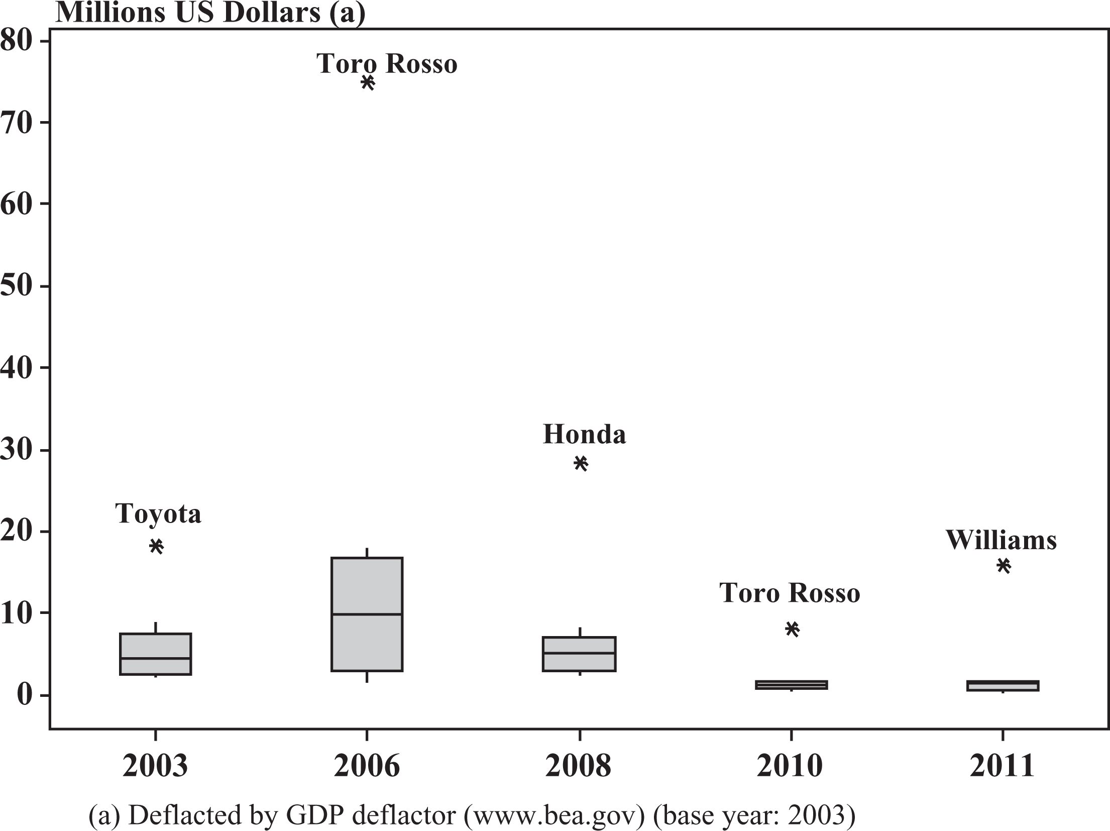
Boxplot of annual budget per point.
Several studies examining the F1 industry have been undertaken in the last years. These studies explore the F1 industry from several perspectives, such as, F1 car designs (Jenkins & Floyd, 2001), practices of intellectual capital (Solitander & Solitander, 2010), estimating the effect of aging on productivity (Castellucci, Padula, & Pica, 2011), public relations strategies (Pfahl & Bates, 2008), and brand profiles (Rosenberger & Donahay, 2008). With respect to efficiency analysis, limited research seems to have been carried out, in spite of efficiency in F1 industry being a relevant issue. The only reference we have found is Carvalho, Figueiredo, Ribeiro, and Correia (2010), which evaluate drivers in the F1 championship using the ELimination Et Choix Traduisant la REalité (ELECTRE II) decision support method considering the pilots of the 2007 season.
This article proposes a method to evaluate constructors’ efficiency in the F1 championship using a well-known nonparametric frontier method, namely data envelopment analysis (DEA). The main goal of this research is to develop a benchmarking procedure that will help F1 fans to identify constructors that excel in terms of their use of financial resources in order to obtain sporting successes. Moreover, analysis of the F1 constructors with the best practices is important for constructors themselves as well as for investors, sponsors, and creditors.
Additionally, F1 currently faces a period of great uncertainty during this harsh recessionary period. This research is justified by the fact that from 2009, an optional budget cap was introduced by FIA, in order to facilitate the entrance of competitors. Participants accepting to operate within the budget cap have the benefit of greater technical freedom than those teams preferring to continue with unlimited budgets, in theory making them more competitive. Budget cap for 2010 season was set to 59.3 millions of dollars per two-car team per season. This budget cap does not include engine costs, drivers, and young driver programmes nor marketing and promotion. In 2010 F1 season, a Resource Restriction Agreement (RRA) was set up by the teams’ association Formula One Team Associations. The compliance of RRA has not been without difficulties so far, particularly in 2011 F1 season.
As it is shown in this article, although there are big differences in the distribution of constructors’ budgets, the corresponding Gini index (GI) is not high, which means that the concentration of the economic resources used in the F1 championship is not as big as supposed. There are more differences, in fact, in terms of performance, with the best-performing constructors gaining a large share of the races and of the points. It is this imbalance between expenditures and results, which suggests the existence of inefficiencies in the way the budgets are spent.
Actually, there are widespread inefficiencies in the industry. The total annual budget excess is over 20% and reached as high as 48% in year 2006. This can be seen as a confirmation of the need to the recent voluntary budget cap. The proposed approach allows the identification of above- and below-average performers. In particular, the few constructors that efficiently manage their budget in each F1 season can be found. No persistent or clear trend is observable in the evolution of efficiency scores, neither at the individual level nor in average. It has been found, however, that all inefficient constructors operate under increasing returns to scale.
The remainder of the article is organized as follows. The second section introduces the DEA methodology and its application to F1 constructors’ efficiency assessment. Third section details the empirical study and presents the results of the efficiency evaluation. Final section summarizes and concludes.
Proposed DEA Approach
DEA is a linear programming technique initially developed by Charnes, Cooper, and Rhodes (1978) to evaluate the efficiency of decision-making units (DMUs) from the observed levels of inputs and outputs. DEA is usually applied to explore the structure of productive efficiency and identify factors that may influence the efficiency. DEA determines a piecewise linear envelopment surface, also referred as the efficient frontier. DMUs that determine the frontier are termed efficient and can be viewed as the “best practice” units relative to the rest of their peers; DMUs that do not lie on the frontier are termed inefficient and the analysis provides measures of their relative efficiencies.
DEA has been applied to the measurement of sport efficiency in many studies; football teams (Barros, Assaf, & Sá-Earp, 2010; Barros & Leach, 2006; Boscá, Liern, Martínez, & Sala, 2009; Espitia-Escuer & García-Cebrián, 2006; García-Sánchez, 2007), baseball (Einolf, 2004; Sueyoshi, Ohnishi, & Kinase, 1999), basketball (McGoldrick & Voeks, 2005), golf (Fried, Lambrinos, & Tyner, 2004), Olympic Games (Lozano, Villa, Guerrero, & Cortés, 2002; Soares de Mello, Angulo-Meza, & Branco da Silva, 2009; Wu, Zhou, & Liang, 2010), and tennis (Ruiz, Pastor, & Pastor, 2011). To our knowledge, this is the first study to investigate the measurement of F1 constructors’ performance using DEA methodology.
The basic features of F1 indicate that it can be studied just like any productive activity. Therefore, it is possible to use the idea of a sports production function, as first proposed by Rottenberg (1956) when discussing baseball. In our case, the efficiency of each constructor is evaluated against this frontier. Hence, the efficiency of a constructor is evaluated relative to the performance of the other constructors.
Consider an F1 season in which there are n constructors, each using m inputs to produce s outputs. Let xij and yrj denote, respectively, the ith (i = 1, 2, . . . , m) input usage and the rth (r = 1, 2, . . . , s) output production of the jth (j = 1, 2, . . . , n) F1 constructor. The input-oriented radial technical efficiency measure, labeled pure technical efficiency, described by Färe, Grosskopf, and Lovell (1985), can be computed with the following linear programming problem:
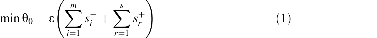
subject to


where λ j is the multiplier of the jth F1 constructor; the minimand θ0 measures the input weak efficiency of the F1 constructor labeled 0, xi 0 represents the variable for the ith input of the assessed constructor 0, yr 0 represents the variable for the rth output of the assessed constructor 0, and ∊ is a non-Archimedean infinitesimal. The slacks values are indicated by s − and s +. Constraining the multipliers to sum to one, as shown in Equation 4 indicates that the efficient frontier can reveal increasing, constant, or decreasing returns to scale; that is, the constraint allows the reference technology to exhibit variable returns to scale (VRS; Banker, Charnes, & Cooper, 1984).
The former model can be reformulated by omitting the constraint Equation 4, thus assuming constant returns to scale (CRS). In this case, the relative efficiency evaluated by the model is the overall efficiency score, labeled technical efficiency, which does not take into account scale effects.
The dual (known as multiplier form) of the Linear Program 1–5 is the following model:

subject to


where u 0 is a scalar associated with Constraint 4 in the primal model.
In this study, initially the proposed model was planned to include one input (i.e., budget) and four performance outputs variables, namely #Points, #Wins, #Podiums, and #Poles. An input orientation is assumed. Hence, in the DEA model proposed, the performance of an F1 constructor is evaluated in terms of its ability to maintain its performance level while reducing its budget subject to the level set by the best-observed practice. If a budget reduction is possible for an F1 constructor, its optimal value θ0 < 1; while if a budget reduction is not possible, the optimal value θ0 = 1. Thus, the implication of the model is that under the assumptions of strong disposability of inputs, and the reference technology exhibiting VRS, for the F1 constructor 0, θ0 gives the fraction to which its budget can be reduced, which means projecting the F1 constructor from the interior of the production possibility set onto the (piecewise-linear) efficient frontier of the production possibility set. The F1 constructor 0 is considered efficient if the efficiency score is equal to one and it has zero slacks. Besides, if the F1 constructor 0 is considered fully efficient in terms of both pure technical efficiency and technical efficiency, it is said to be operating in the most productive scale size (Banker, 1984). The scale efficiency can be measured by the ratio of the CRS efficiency score to the VRS efficiency score, that is, the ratio of the technical efficiency to the pure technical efficiency.
In this study, DEA procedure was used, first, because of its nonparametric character. Second, although the discriminatory power of DEA models increases with sample size (Zhang & Bartels, 1998), the uses of DEA is justifiable because it offers, even with small samples, more accurate efficiency scores than other parametric methodologies (Banker, Gadh, & Gorr, 1993). In the case of F1 constructors, since it is not large, the whole F1 constructors’ population is assessed.
Assessment of F1 Constructors’ Efficiency
This section evaluates the performance of the F1 constructors during 2003, 2006, 2008, 2010, and 2011 seasons. First, the potential of the constructors and their results are compared not by considering their efficiency in the use of resources, but by observing their final table positions. Second, the technique which is used to estimate the frontier is DEA, which has not been so far for efficiency assessment in the F1 World Championship literature.
The Data Set
The analysis was made considering the constructors that competed in the FIA Formula One World Championship for past F1 seasons and it includes all the different constructors for each season considered. We only select those constructors that complete the F1 season. The required information was obtained from the FIA official website (http://www.fia.com).
The data used to study the determinants of efficiency analysis consists of 2003, 2006, 2008, 2010, and 2011 F1 seasons as given in Table 1. Although data of other remaining years would ideally be incorporated in the study, data availability constraints prevented such complete analysis. The number of participating constructors in those seasons was 10, 11, 11, 12, and 12 for 2003, 2006, 2008, 2010, and 2011, respectively. Constructors are not the same across the seasons however. Thus, for instance, although in partnership with B.A.R. from year 2000, Honda did not return to World Constructors’ Championship until 2006. Similarly, Sauber left the F1 competition after 2003 F1 season, reentering in 2011 F1 season. Also, incorporations to the F1 competition have taken place in the last two seasons. Red Bull and Force India joined as competitors in F1 racing in 2008 and 2005, respectively. More recently, Lotus, Mercedes (from Mc Laren split), HRT, and Virgin were the newest additions to the grid in 2010 F1 season.
Input and Output Data of Participants in F1 World Constructors’ Championship.
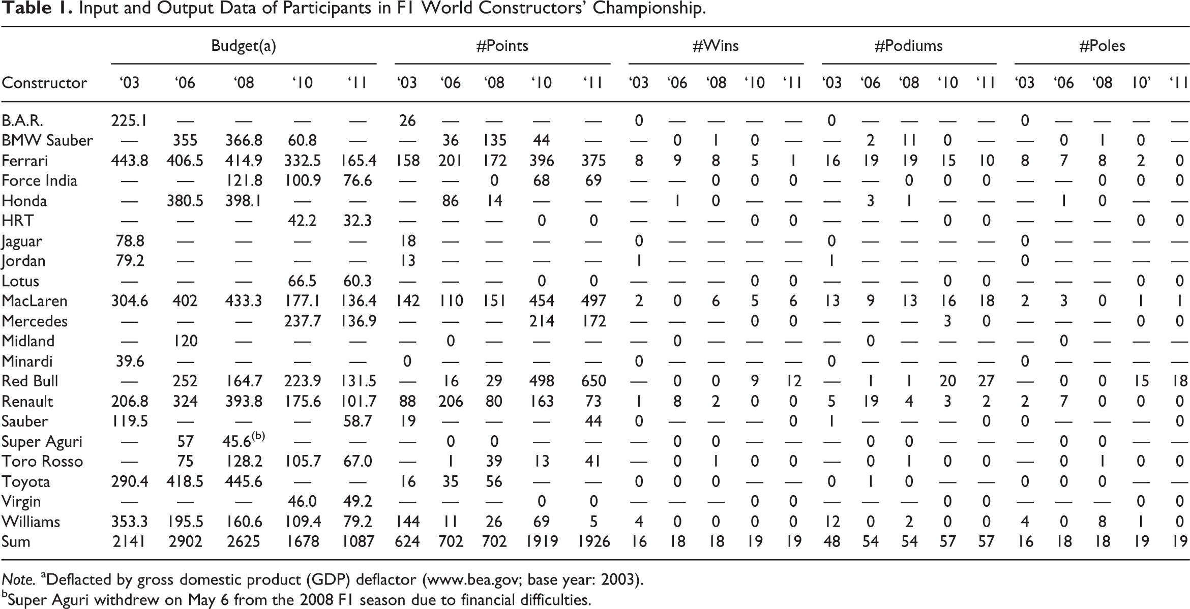
Note. aDeflacted by gross domestic product (GDP) deflactor (www.bea.gov; base year: 2003).
bSuper Aguri withdrew on May 6 from the 2008 F1 season due to financial difficulties.
One of the teams’ resources is the budget for each season. Although the precise details of constructors’ budgets are not revealed by the FIA, estimates (measured in millions of U.S. dollars and expressed in real prices) can be found in F1 magazines and web sites specializing in F1. The total operating budget includes spending categories such as engines budget, operating the cars at tests, team salaries, operating the cars at races, research and development, drivers salaries, wind tunnel operating costs, travel and accommodation, corporate entertaining and catering, and car manufacturing costs.
In order to evaluate the concentration degree of the constructors’ budgets, the concentration curve comparing the cumulative percentage of constructors (Fi ), up to the ith constructor, versus the cumulative percentage of budget spent by those same first i constructors (Qi ) for each F1 season is represented in Figure 2. The uniform (i.e., equal) budget distribution is represented by the diagonal line. The smaller the area between the concentration curve and the diagonal, the smaller the concentration is. The GI is calculated, ranging between .21 (with a corrected upper bound GImax = .83) in 2008 F1 season and .31 (with a corrected upper bound GImax = .84) in 2010 F1 season. The highest value of concentration of budget over the F1 seasons is relatively low which means that the industry budget is not very concentrated, that is, there is not excessive concentration in terms of the economic resources used by the different constructors. On average, half of the largest constructors spend just 70% of the total industry budget. Finally, there is no clear trend in the concentration level over the F1 seasons under study.
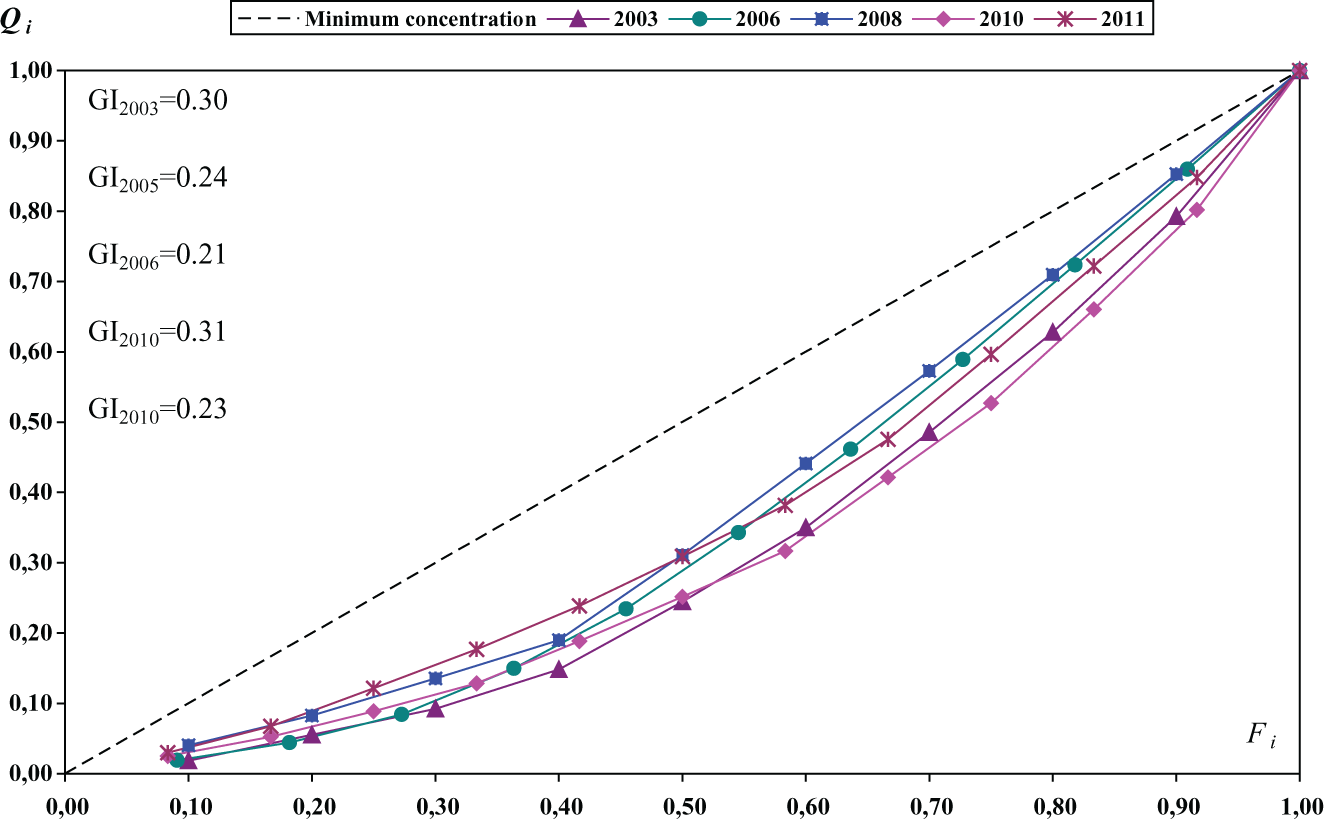
Concentration curve and Gini Indexes (GI).
As a measure of performance, we considered the total number of points awarded (#Points), number of wins (#Wins), number of times on the podium (#Podiums), and number of poles (#Poles) reached by each constructor at the end of the season. The 2003 season covered 16 races; the 2006 and 2008 seasons covered a total of 18 races each, while 2010 and 2011 seasons covered 19 races each.
It can be observed, in Table 1, that budget data (expressed in 2003 constant U.S. dollars) are not uniformly distributed. Some constructors are very large in terms of budget while others are relatively small. For instance, Toyota had almost 10 times as much to spend in the 2008 F1 season as Super Aguri and Ferrari had almost 8 times to spend in 2010 F1 season as HRT. The data set contains three large constructors, which together won around 62%, 57%, 73%, 70%, and 79% of the total points in the final classification of 2003, 2006, 2008, 2010, and 2011 F1 seasons.
Originally, the DEA model considered included five variables (one input and four outputs as shown in Table 1). Unfortunately, in our case, this number of variables is large relative to population of constructors. In general, the total number of variables in the DEA model should be no more than one third of the number of DMUs under assessment (Sinuany-Stern & Barboy, 1994). In our study, this assumption is not verified. To overcome this, and given the evident high correlation between the output variables, a method for selection of the most informative output variables has been applied (Cadima & Jollife, 2001). This method identifies subsets of variables that best approximate the full set of variables, thus stressing dimensionality reductions in terms of the original variables rather than in terms of derived variables, as in methods based on principal components (PC), whose definition require all the original variables. The selection of variable subsets is based on indicators of the performance of different subsets of the variables using Yanai’s generalized coefficient of determination (GCD; Cadima & Jollife, 2001; Ramsay, ten Berge, & Styan, 1984). This criterion, defined by expression (10), measures the closeness between the orthogonal projections onto the subspace spanned by the first q PC’s using a subset of k variables (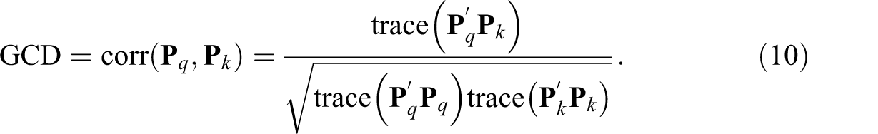
The GCD criterion lies between zero, in case the subspaces are orthogonal, and one, in case all k PCs are in the subspace spanned by the k variables. Suitable for our small-size data set, an exact algorithm for optimizing the above criteria based on Furnival and Wilson’s leaps-and-bounds algorithm for variable selection in regression analysis (Duarte Silva, 2001, 2002) is employed.
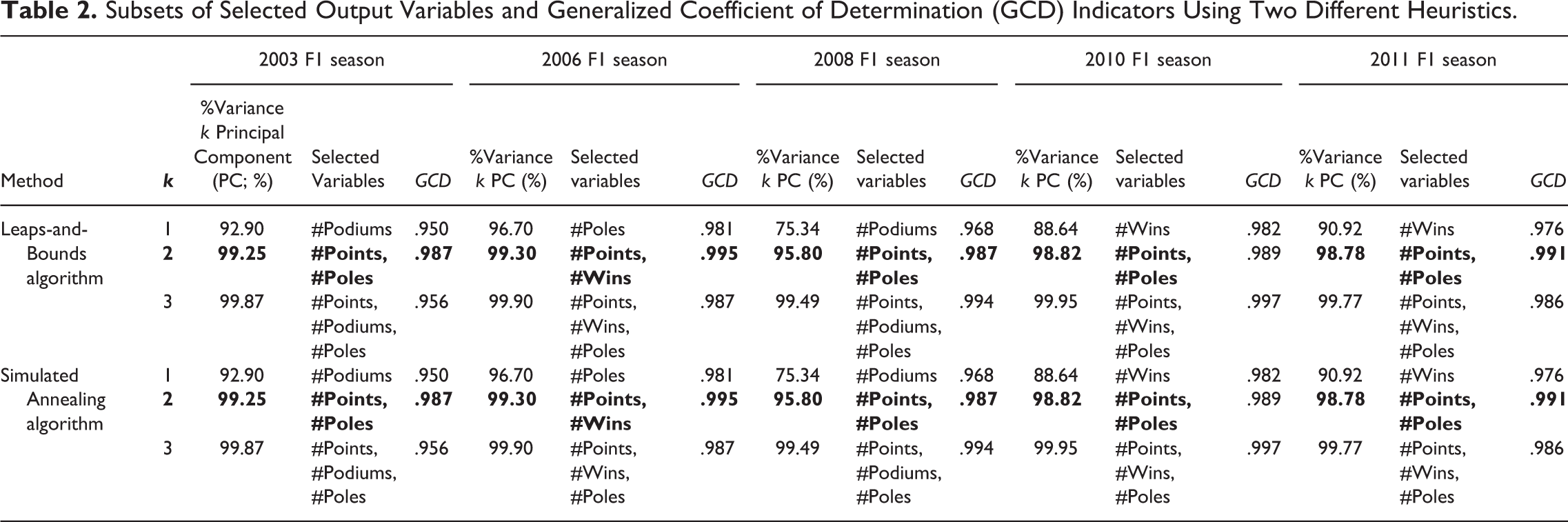
Table 2 shows the results of the GCD approach. For each season, the percentage of the data variance that is explained by the first k PC and the GCD of the optimal subset are presented. Note that as the number of indicators selected k increases so does the percentage of variance explained. The inclusion of the four output variables suggests that there may be redundancy in the data and that most of the information and structure could be retained using fewer variables. This is supported by the fact that the first two PC of the data account for about 95.8% of the total variation for 2008 F1 season, this being figure even higher in the other F1 seasons. The GCD criterion results are listed in Table 2 and are used to evaluate retaining subsets of size 1, 2, and 3. This procedure suggests retaining a value of k so that the first k PC explains approximately 90% of variance and the indicator of subspace similarity grows for a different subset of k variables. This means, in 2008 F1 season, selecting, from the four variables, the subset corresponding to row k = 2, two-variable subset, (i.e., #Points and #Poles), which is the subset optimal for the GCD indicator. Similarly, in 2003, 2006, 2010, and 2011 F1 seasons, only one variable need to be retained, that is, #Podiums (’03), #Poles (’06), #Wins (’10, ’11). The GCD between the subspaces spanned by the first PC and the variable selected using the leaps-and-bounds and the simulated annealing algorithms are coincident and range, for the seasons considered, from .95 to .98 for k = 1, .98 to .99 for k = 2, and .95 to .99 for k = 3. For comparison purposes, the same number of output variables is selected, that is, k = 2, for the five seasons (row highlighted in bold). Additionally, since the redundant output variables coincide in 2003, 2008, 2010, and 2011 F1 seasons, that is, #Podiums and #Wins, the output variables considered in the DEA model will be #Points and #Poles for all F1 seasons.
Subsets of Selected Output Variables and Generalized Coefficient of Determination (GCD) Indicators Using Two Different Heuristics.
Efficiency Scores Analysis
The efficiency scores resulting from DEA for all constructors and for each season were obtained using the input-oriented, VRS DEA Model 1–5, known as BCC DEA model. The model was solved also assuming CRS, known as CCR DEA model (Charnes, Cooper, & Rhodes, 1978), that is, without Constraint 4, thus calculating the technical efficiency, which does not take scale size effects into account.
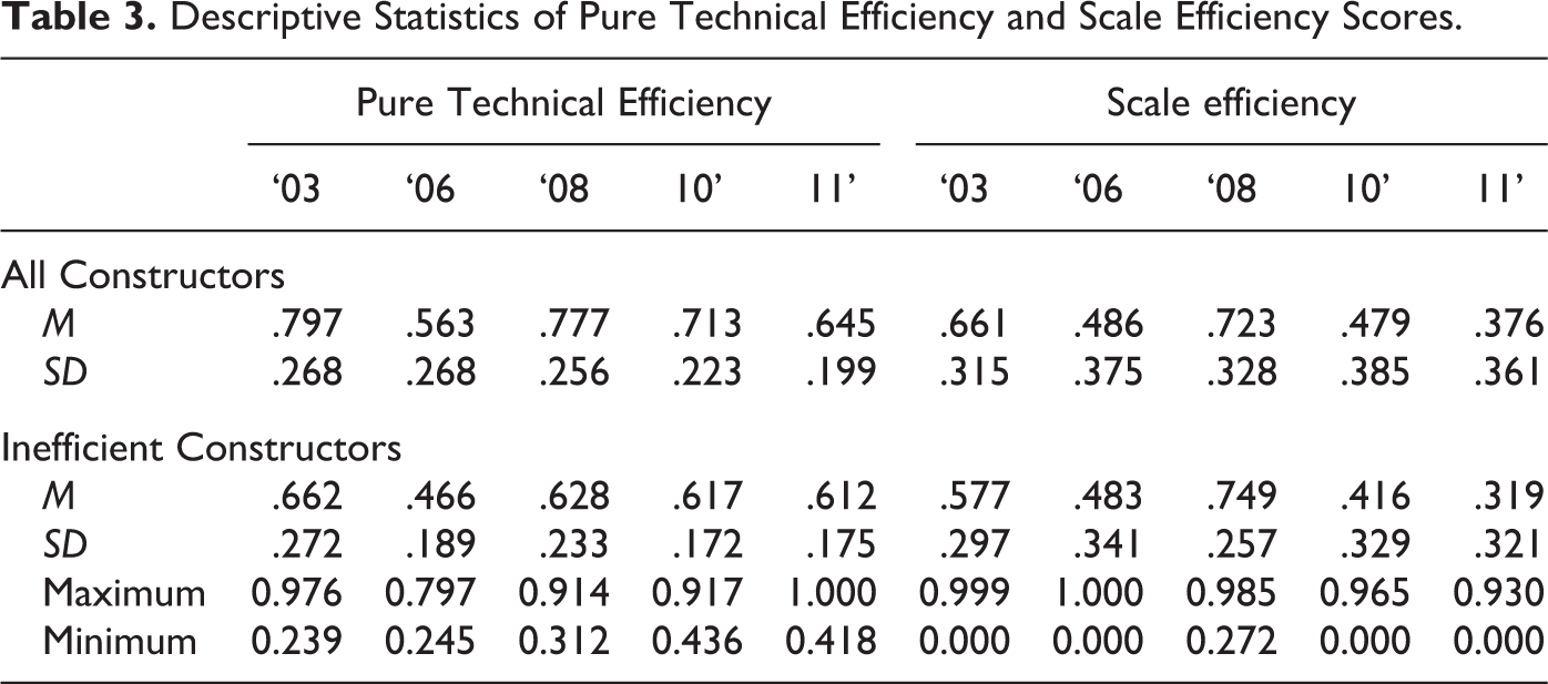
The results of the BCC model and summary statistics of calculated values of the efficiency measures in 2003, 2006, 2008, 2010, and 2011 F1 seasons are presented in Table 3. The average technical efficiency of the F1 constructors differs across the seasons. A sharp decline in average efficiency from about .79 in 2003 F1 season to about .56 in 2006 F1 season is detected. Nonetheless, increased average technical efficiency scores took place in the following F1 seasons. A significant dispersion in the efficiency of the different constructors across the five seasons can be observed. Note, also, that the minimum technical efficiency score increased across the F1 seasons considered.
Descriptive Statistics of Pure Technical Efficiency and Scale Efficiency Scores.
The results of the BCC and CCR DEA models in 2003, 2006, 2008, 2010, and 2011 F1 seasons are graphically shown in Figure 3a–e, respectively. The graphs coordinates (x axis, y axis) are the pure technical efficiency score and the technical efficiency score, respectively. Efficient constructors appear in italics and are located on the point (1,1) in Figure 3. The horizontal line in each figure displays the average technical efficiency, while the vertical line represents the average pure technical efficiency. These two lines allow an easy identification of the constructors with above- or below-average efficiency scores. The straight line with Slope 1 describes scale efficiency, that is, the technical efficiency score of a given constructor (computed under CRS) is equal to the pure technical efficiency (computed under VRS).
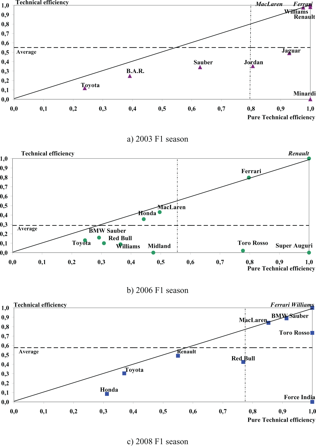
Technical efficiency versus pure technical efficiency. (a) 2003 F1 season. (b) 2006 F1 season. (c) 2008 F1 season. (d) 2010 F1 season. (e) 2011 F1 season.
The technical and pure technical efficiencies of F1 constructors for the 2003 season are plotted in Figure 3a. The average technical efficiency (.55) and average pure technical efficiency (.80) are also shown as references. Two constructors were found efficient (namely Ferrari and MacLaren) with MacLaren referenced 6 times as benchmark to inefficient constructors. Ferrari and MacLaren operated at the most productive scale size (Banker, 1984). These two constructors efficienctly exploited their budgets to reach their observed performance results. In 2003, Williams and Renault had very high efficiency scores compared to the other inefficient F1 constructors.
Different clusters of constructors can be identified in 2006 and 2008 F1 seasons as shown in Figure 3b and c, respectively. Renault is the only technical efficient constructor in the 2006 F1 season and it was referenced 7 times as benchmark by its peers. During the F1 2008 season, Ferrari and Williams operated at the most productive scale size. This is an interesting result, given the differences with respect to the relative sizes of the budget of both constructors that year (414.9 vs. 160.6).
Although not shown in the tables, for lack of enough space, the results of the study show that, if we focus in the most recent seasons, 2010 and 2011, BMW Sauber, Ferrari, Force India, HRT (’11), Lotus (’11), Mercedes, Renault, Sauber (’11), Toro Rosso (’11), Virgin (’11), and Williams had pure technical efficiency scores higher than the corresponding scale efficiency scores. That means that the overall inefficiencies of the referred constructors are primarily due to the scale inefficiencies. Thus, HRT had pure technical efficiency scores equal to 1 but the scale efficiency scores less than 1. They can possibly increase their operation scales to improve their overall efficiencies. On the other hand, the rest of inefficient constructors are mainly lacking in technical efficiency. Additionally, Ferrari, Mercedes, and Renault (’10) belong to a group of constructors with low technical efficiency and high scale efficiency, which means that they have relatively large budgets for their observed performance results. Summing up, all the inefficient constructors exhibited Increasing Returns to Scale, except for the efficient constructors that operate at CRS.
In examining the detailed results, some additional points emerge. First, the highest levels of inefficiency occurred in the 2006 F1 season; as it can be observed in Table 3, the average efficiency of inefficient is very low (.46). The second major finding is that half of the efficiency losses are scale and the other half technical inefficiency. It can be also noted that Ferrari is the only scale efficient constructor during each of the 2003, 2006, and 2008 F1 seasons and Red Bull in both the 2010 and the 2011 F1 seasons. Nevertheless, Ferrari was identified as pure technical inefficient in 2006, 2010, and 2011 F1 season, its pure technical efficiency declining in the last season to .52.
Budget Reduction Analysis
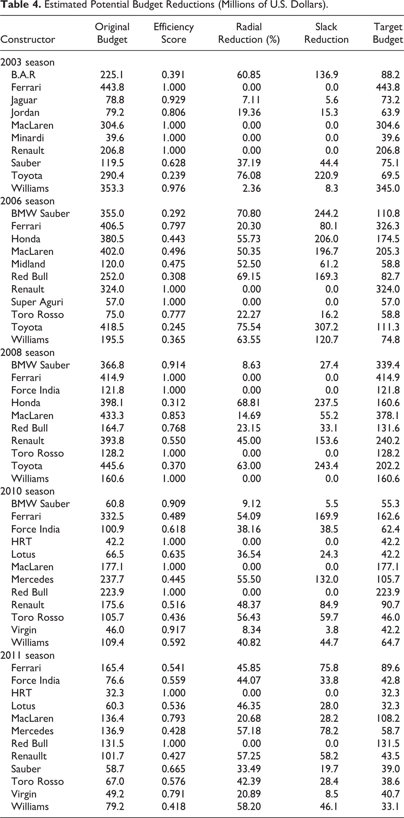
In order to explain constructors’ efficiency scores, it is helpful to look at their potential budget reduction. These are shown in absolute as well as in relative terms in Table 4. According to the input slack values, the inefficient constructors can reduce their budget to reduce their inefficiencies and become efficient constructors. It is remarkable that for each season more than half of constructors could reduce their budget. Across the period considered, the industry total budget excesses ranges from 404.88 million of U.S. dollars in 2011 (37.2% of the total budget) to a maximum of 1401.9 million of U.S. dollars in 2006 (a staggering 48.3% of total budget). Toyota had the highest potential budget reduction in 2003 and 2006 F1 seasons. In the 2008 F1 season, Honda had the highest excess budget, approximately 69%; also close to this figure that same year was Toyota (63%). In the last F1 season (year 2011), apart from Red Bull and HRT, which were pure technical efficient, the constructors with the lowest budget excesses in absolute terms have been Virgin (8.54 million US$) and Sauber (19.66 million US$) and, in relative terms, Virgin (20.89% of budget excess) and MacLaren (20.26% budget excess).
Estimated Potential Budget Reductions (Millions of U.S. Dollars).
Conclusions
In F1 racing sport, a period of increased uncertainty is coming up due to changes due to the introduction of a voluntary budget cap. According to FIA, a creative technical competition is part of F1’s identity, but in an environment of strong, responsible, and innovative management, not based on a spending race. Based on efficiency analysis, this study investigated F1 competition from constructor’s perspective to gauge their relative performance. DEA methodology is used to measure constructors’ managerial efficiency using budget as input, and F1 racing performance results. The constructors are heterogeneous in terms of size; hence VRS are assumed for the production possibility set.
This empirical study has shown that inefficient constructors have low efficiencies on average across the different F1 seasons. Substantial budget reductions should have to be done by inefficient constructors in order to be efficient as the identified as benchmarks. The overall industry budget excess ranges from 20% to a maximum (in year 2006) of almost 50%. It seems that there has been much overspending in these years, which justifies the need for the recently introduced voluntary budget cap.
It can be noted that constructors’ relative efficiency varies across the five seasons considered. The proposed approach allows the identification of above- and below-average performers in each F1 season. In general, only a few (two at most) have been assessed as efficient in a specific F1 season. In 2003, 2006, and 2008 F1 seasons, high-efficiency constructors (03’—Ferrari, MacLaren; 06’—Renault; 08’—Ferrari, Williams) as well as low-efficiency constructors (03’—Minardi, Toyota; 06’—Midland, Super Aguri; 08’—Force India, Honda) are identified. On average, Ferrari and MacLaren have significant higher efficiency scores compared to the constructors’ average in 2003, 2006, and 2008 F1 season. In the most recent 2010 and 2011 F1 seasons, Red Bull and MacLaren occupy the top performance position. In general, constructors showed a favorable evolution of their efficiency during the five seasons considered. On the other hand, in terms of scale size, all inefficient constructors presented Increasing Returns to Scale in all five seasons F1 considered.
Finally, mention should be made to drawbacks and limitations of the study. One is the fact that the budget figures used are estimates and not official figures since the latter are, understandably, not available due to the high-stakes, secretive nature of this business. In addition, although the data used cover the most important economic and performance variables, many other important aspects related to safety and environmental impact have not been considered due to data unavailability. Nonetheless, this remains an interesting topic for further research. Further research could also extend the DEA methodology to other motorsports, such as NASCAR Sprint Series Cup or Indy Racing League, and evaluate also the performance of the drivers or team leaders.
Footnotes
Declaration of Conflicting Interests
The author(s) declared no potential conflicts of interest with respect to the research, authorship, and/or publication of this article.
Funding
The author(s) received no financial support for the research, authorship, and/or publication of this article.