Wage Disparity and Team Performance in the Process of Industry Development

Abstract

The changing effects of wage disparity on team performance during the process of industry development are examined using data sourced from the Japanese professional football league. The results show that wage disparity leads to a reduction in team performance during the developing stage but does not influence performance during the developed stage. Unobserved fixed team effects and endogeneity bias were controlled in the study.

Keywords

wage disparity team performance industry development

Introduction

Two conflicting views exist regarding wage disparity within sports teams and its effect on team performance in professional leagues. One theory purports that wage equality improves team performance and will, therefore, enhance worker cooperation (Levine, 1991). There are a number of studies that support this view (e.g., Depken, 2000; Richards & Guell, 1998; Sommers, 1998; Wiseman & Chatterjee, 2003). In contrast, tournament theory suggests that wage inequality leads to higher worker productivity (Lazear & Rosen, 1981; Rosen, 1986).¹ If this is true, wage inequality improves team performance, which is also supported by empirical evidence (Avrutin & Sommers, 2007).²

Previous studies have not considered endogeneity in wage inequality, and so their results appear to exhibit estimation bias. This article attempts to control for this bias using the dynamic panel model. Furthermore, the effect of wage inequality on team performance possibly depends on the conditions within professional sports leagues, an aspect that has not been sufficiently investigated. For instance, the skill level of professional sports leagues can appear low during inception stages, and then improve over time, through experience and technology transfers from more advanced foreign leagues (Yamamura, 2009). During this development process, the effect of income inequality on team performance may change. Using data sourced from the Japanese professional football league (J-League), established in 1993, this article examines the relationship between wage inequality and team performance in the context of industry development.

Data and Model

Approximately 200 countries belong to the Fédération Internationale de Football Association (FIFA), while only 32 teams, those that win preliminary rounds, are able to participate in the final tournament. Since Japan’s J-League began in 1993, the skills and performance of the Japanese national team have improved significantly. This improvement is due in part to the transfer of star players, from professional football leagues in South America and Europe, into the J-league. For example, Zico (Brazil) and Schillaci (Italy) played in the J-league during its early stages. Prior to 1993, the Japanese national team consisted of amateur players and its performance had been far from the level required to advance to the World Cup. In 1994, the Japanese team comprised J-League players but failed to qualify for the Football World Cup. However, 4 years later, the Japanese team won its preliminary competition and qualified to play in the 1998 World Cup. Subsequently, the Japanese team has qualified for the last three World Cups (2002, 2006, and 2010).³

Team-level data regarding the J-league were used to examine how the effects of wage disparity on team performance vary at different team-development stages. This article uses a data panel to describe the J-league teams from 1993 to 2011. Team-level data were constructed based on a large player sample containing approximately 12,000 observations. Data were sourced from the Nikkan Sports newspaper from 1994 to 2012. To conduct the estimation (using data from 1993 to 2011), the sample was divided into developing and developed stages, and the effects of wage disparity on team performance during the different stages were compared. The period 1993–1997 is defined as the developing stage because during this period Japan did not qualify to play in the World Cup, while the period 1999–2006 is defined as the developed stage, after Japan’s 1998 World Cup qualification. However, it is possible that Japan had not attained the necessary skills and techniques required in the developed stage despite qualifying for the World Cup as Japan lost every game in the 1998 World Cup.⁴ However, it was thought that Japan would learn from the experience of participating in the World Cup and then further cultivate their ability. In the next World Cup held in Japan and Korea, Japan won two games against Tunisia and Russia. Thus, there appears to be a time lag between the 1998 World Cup qualification and when Japan actually reached the developed stage. The definition of developing and developed stages may vary among researchers and it is difficult to exactly define these periods. Further, estimation results are possibly influenced by the definitions used for the developing stage and developed stage. Hence, for a robustness check, alternatively defined periods are also used as the developing and developed stages. That is, the periods 1993–1998, 1993–1999, 1993–2000, and 1993–2001 are also defined as the developing stage, and the periods 1999–2011, 2000–2011, 2001–2011, and 2002–2011 are also defined as the developed stage.

Table 1 includes the variable definitions and a summary of statistics. As in Depken’s (2000) study on baseball, a fixed effects model was also used in this study, with WIN as a dependent variable, and AVSAL, SALHHI, AVAGE, and SDAGE as independent variables and year dummies. In addition to the salary of players, the age of players is thought to affect team performance because their physical condition and experience change over time. Hence, AVAGE and SDAGE are incorporated as control variables. Because of limited data, other variables cannot be incorporated as independent variables. However, AVSAL and SALHHI are considered endogenous variables, which create endogeneity bias due to the reverse causality that team performance influences players’ salaries and the accompanying wage disparity within a team.⁵ In addition to the fixed effects model, a Arellano-Bond type dynamic panel model (Arellano, 2003) is used in this article for the purpose of controlling for endogeneity bias and unobservable fixed team effects. This article provides a control for endogeneity bias, a measure not taken in earlier studies (e.g., Avrutin & Sommers, 2007; Berri & Jewell, 2004; Depken, 2000; Richards & Guell, 1998; Sommers, 1998). The estimated function takes the following form:

Table 1.

Descriptive Statistics of Study Data (1993–2011).

	Definition	M	SD	Minimum	Maximum
WIN	Rate of wins	0.45	0.15	0.86	0.11
AVSAL	Average annual salary of players (million yen)	2.30	0.98	6.24	0.56
SALHHI	Inter-team annual salary: Herfindahl index	0.07	0.05	0.56	0.03
AVAGE	Average age of players	24.9	1.01	28.1	22.3
SDAGE	Standard deviation of age of players	4.35	0.52	5.95	3.08

\begin{aligned} {W I N}_{i t} & = α_{1} {W I N}_{i t - 1} + α_{2} {A V S A L}_{i t} + α_{3} {S A L H H I}_{i t} + α_{4} {A V A G E}_{i t} + α_{5} {S D A G E}_{i t} \\ + ε_{t} + ν_{i} + u_{i t}, \end{aligned}

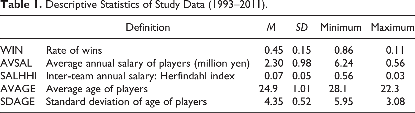
where ∊ _t , ν _i , and u_it represent the following unobservable effects: ∊ _t , is the year-specific effects, ν _i , is the unobserved team-specific effects, and u_it is the error term, respectively. t−1 is the lagged year of the t year. The structure of the data set used in this study is panel form. Lagged dependent variable WIN _it− ₁ was used as a control in the initial level. AVSAL and SALHHI were used as endogenous variables in the dynamic panel model and the levels of endogenous variables that lagged for two or more periods could also be used as instrumental variables (Arellano, 2003).

Results

Using data from 1993 to 2011, Table 2 shows the results from the fixed effect and dynamic panel model estimations. A fixed effects model was also used by Depken (2000) in a study on major league baseball. In columns (1) and (2), the results of the fixed effects model are presented, while those of the dynamic panel model are presented in columns (3) and (4). Further, year dummies are included in columns (1) and (3), whereas year dummies are not included in columns (2) and (4). Table 2 (column 3) and (column 4) illustrates Sargan’s overidentification test and second-order serial correlation test used to check the validity of the estimation results in the dynamic panel model. The null hypothesis is that the instrumental variables do not correlate with the residuals. If the hypothesis is not rejected, the instrumental variables are valid. Further, the test for the null hypothesis (that there is no second-order serial correlation with the disturbance of the first-differenced equation) is important because the estimator is consistent when there is no second-order serial correlation. Table 2 (column 3) and (column 4) shows that the hypothesis that the instrumental variables do not correlate with the residuals is rejected in columns (3) and (4), suggesting that the estimation results are invalid. Hence, careful attention should be called for when the results of columns (3) and (4) are interpreted. In this article, I focus on the results of the key variable SALHHI. Table 2 shows that SALHHI takes a negative sign and is statistically significant in columns (1) and (2), which is congruent with the results from Depken’s (2000) major league baseball study. However, columns (3) and (4) show the negative sign but are not statistically significant, which is not consistent with Depken’s findings. These results show that the choice of estimation model influences the results for SALHHI. In addition, AVSAL yields the positive sign in all columns and is statistically significant with the exception of column (3). This indicates that players with high salaries contribute to a team’s wins. Players with good performance earn high salaries, resulting in a high winning rate. Concerning the age of players, AVAGE and SDAGE are not statistically significant in any estimation. Hence, the age of players is not associated with team wins.

Table 2.

Determinants of Winning Ratio for Whole Period (1993–2011).

	(1)	(2)	(3)	(4)
	Fixed Effects	Fixed Effects	Dynamic Panel	Dynamic Panel
WIN _it ₋₁			0.22*** (2.82)	0.30*** (3.27)
AVSAL _it	0.05*** (4.30)	0.06*** (5.86)	0.01 (0.59)	0.03*** (3.53)
SALHHI _it	–0.52* (–1.95)	–0.66*** (–3.96)	–0.14 (–0.29)	–0.46 (–0.77)
AVAGE _it	–0.001 (–0.04)	–0.01 (–1.37)	0.01 (0.91)	–0.01 (–1.02)
SDAGE _it	–0.01 (–0.80)	–0.01 (–0.71)	–0.001 (–0.04)	–0.01 (–0.43)
Year dummies	Yes	No	Yes	No
Sargan test			210	210
(p value)			(.07)	(.07)
Serial correlation			–0.15	−0.15
Second order			(.87)	(.87)
(p value)
Observations	309	309	226	226

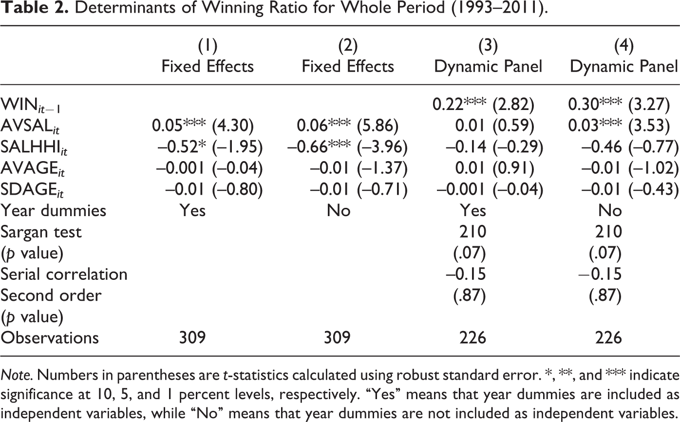
Note. Numbers in parentheses are t-statistics calculated using robust standard error. *, **, and *** indicate significance at 10, 5, and 1 percent levels, respectively. “Yes” means that year dummies are included as independent variables, while “No” means that year dummies are not included as independent variables.

Table 3 provides the results of the fixed effects estimation. Table 3 (column 1) presents results based on data from the developing stage, and Table 3 (column 2) presents results based on data from the developed stage. Table 4 provides the results of the dynamic panel estimation. Table 4 (column 1) presents results based on data from the developing stage, and Table 4 (column 2) presents results based on data from the developed stage. In Tables 3 (column 1) and 4 (column 1), results for 1993–1997, 1993–1998, 1993–1999, 1993–2000, and 1993–2001 are exhibited in columns (1), (2), (3), (4), and (5), respectively. In Tables 3 (column 2) and 4 (column 2), results for 1998–2011, 1999–2011, 2000–2011, 2001–2011, and 2002–2011 are exhibited in columns (1), (2), (3), (4), and (5), respectively.

Table 3.

Determinants of Winning Ratio (Fixed Effect Model).

The Developing Stage
	(1)	(2)	(3)	(4)	(5)
	1993–1997	1993–1998	1993–1999	1993–2000	1993–2001
AVSAL _it	0.01 (0.77)	0.02 (1.09)	0.02 (1.71)	0.03* (1.83)	0.03** (2.13)
SALHHI _it	–0.72** (–2.38)	–0.76** (–2.27)	–0.57** (–2.17)	–0.59** (–2.13)	–0.62** (–2.16)
AVAGE _it	–0.01 (–0.77)	–0.02 (–1.03)	–0.01 (–0.32)	–0.004 (–0.23)	0.003 (0.16)
SDAGE _it	0.09 (1.53)	0.08* (2.04)	0.04 (1.32)	0.02 (0.89)	0.01 (0.43)
Less developed group vs. developed group
Chow test	F = 3.82	F = 5.05	F = 4.44	F = 5.44	F = 3.84
(p value)	(.01)	(.00)	(.00)	(.00)	(.01)
Observations	69	87	103	119	135
The Developed Stage
	(1)	(2)	(3)	(4)	(5)
	1998–2011	1999–2011	2000–2011	2001–2011	2002–2011
AVSAL _it	0.04 (1.60)	0.05* (1.95)	0.04 (1.26)	0.04 (1.01)	0.01 (0.35)
SALHHI _it	1.06 (1.67)	0.86 (1.23)	0.88 (1.34)	0.93 (1.49)	0.62 (1.14)
AVAGE _it	0.01 (1.17)	0.01 (0.66)	0.01 (0.59)	0.01 (0.92)	0.01 (0.96)
SDAGE _it	–0.02 (–1.11)	–0.03 (–1.57)	–0.03* (–1.78)	–0.02 (–1.19)	–0.02 (–1.27)
Observations	240	222	206	190	174

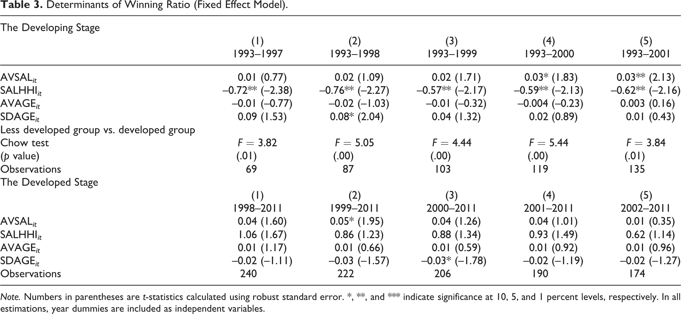
Note. Numbers in parentheses are t-statistics calculated using robust standard error. *, **, and *** indicate significance at 10, 5, and 1 percent levels, respectively. In all estimations, year dummies are included as independent variables.

Table 4.

Determinants of Winning Ratio (Dynamic Panel Model).

The Developing Stage
	(1)	(2)	(3)	(4)	(5)
	1993–1997	1993–1998	1993–1999	1993–2000	1993–2001
WIN_it− ₁	0.14 (0.83)	0.03 (0.24)	0.04 (0.32)	0.06 (0.75)	–0.01 (–0.24)
AVSAL _it	0.04 (0.72)	0.04 (0.78)	0.01 (0.56)	0.02 (0.85)	0.03 (1.25)
SALHHI _it	–2.08** (–2.06)	–2.23** (–2.15)	–1.28* (–1.72)	–1.52** (–2.24)	–1.51** (–2.11)
AVAGE _it	–0.01 (–0.46)	–0.01 (–0.43)	0.01 (0.45)	0.01 (0.39)	0.02 (0.83)
SDAGE _it	0.09** (2.33)	0.06* (1.94)	0.05 (1.37)	0.04 (1.38)	0.01 (0.49)
Sargan test	15.1	26.2	47.8	57.3	73.4
(p value)	(.36)	(.33)	(.09)	(.19)	(.13)
Serial correlation	–1.00	–0.77	–1.17	–1.59	–2.05
Second order	(.31)	(.43)	(.23)	(.11)	(0.04)
(p value)
Observations	36	52	68	82	95
The Developed Stage
	(1)	(2)	(3)	(4)	(5)
	1998–2011	1999–2011	2000–2011	2001–2011	2002–2011
WIN_it− ₁	0.21** (2.39)	0.29*** (3.83)	0.24*** (2.65)	0.22** (2.38)	0.23** (2.11)
AVSAL _it	0.003 (0.13)	0.03 (1.22)	0.006 (0.21)	0.01 (0.49)	0.01 (0.33)
SALHHI _it	0.96** (2.33)	0.49 (0.79)	0.81 (1.37)	0.91* (1.65)	0.38 (0.62)
AVAGE _it	0.02** (1.99)	0.001 (0.42)	0.02 (1.27)	0.01 (0.77)	–0.04 (–0.21)
SDAGE _it	–0.01 (–0.65)	–0.03 (–1.24)	–0.03 (–1.35)	–0.03 (–1.55)	–0.03 (–1.44)
Sargan test	198.4	180.1	164.8	142.3	135.6
(p value)	(.04)	(.09)	(.09)	(.19)	(.11)
Serial correlation	–0.04	0.58	1.15	0.76	1.40
Second order	(.96)	(.55)	(.24)	(0.44)	(.15)
(p value)
Observations	190	174	158	144	131

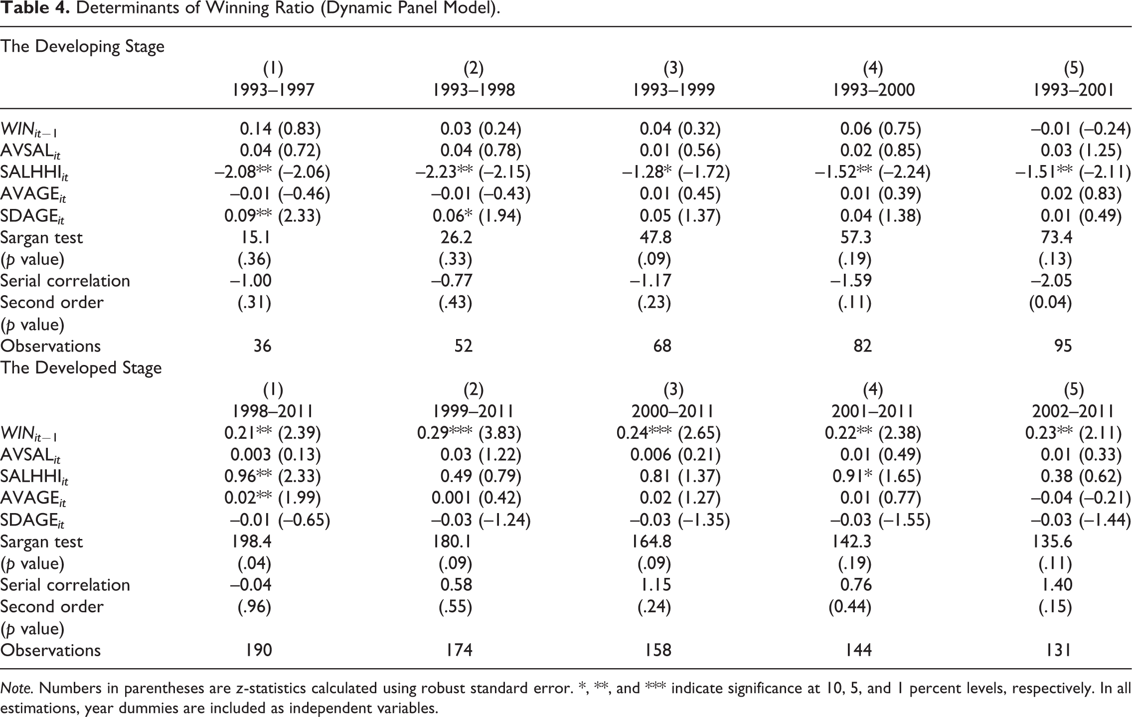
Note. Numbers in parentheses are z-statistics calculated using robust standard error. *, **, and *** indicate significance at 10, 5, and 1 percent levels, respectively. In all estimations, year dummies are included as independent variables.

A Chow test was conducted to check for structural change. That is, F statistics were used to test that the restrictions on the coefficients of AVSAL, SALHHI, AVAGE, and SDAGE in two equations (results for the developing stage and the developed stage) are the same. The results of the Chow test are reported in Table 3 (column 1) and show that the hypothesis, that the regression model is the same for the two periods, is rejected in all columns. That is, the data suggest that the models for the two periods are systematically different. In line with the conjecture explained earlier, the structure of the J-League in the developing stage is considered different from that in the developed stage. Table 3 (column 1) shows that the coefficient of SAHHI produces the negative sign and is statistically significant in all columns. This implies that wage disparity leads to a reduction in team performance during the developing stage. AVSAL has a positive sign in all columns, and it is not statistically significant in columns (1)–(3). Hence, the positive effect of AVSAL on the winning ratio is not robust. AVAGE and SDAGE are not statistically significant with the exception of SDAGE in column (2). Turning to the developed stage in Table 3 (column 2), SALHHI has a positive sign in all estimations. However, SALHHI is not statistically significant in any column. That is, the negative effect of wage disparity disappears in the developed stage. Concerning other control variables, they are not statistically significant with the exception of AVSAL in columns (2) and SDAGE in column (3).

Table 4 shows the results for Sargan’s overidentification test and second-order serial correlation test. Table 4 (column 1) and (column 2) shows that both hypotheses are not rejected in the majority of the estimations, suggesting that the estimation results are valid. Interestingly, in Table 4(1), SALHHI continues to yield a negative sign and is statistically significant in all columns. The coefficient of the lagged dependent variable WIN _it ₋₁ has a positive sign but is not statistically significant in all columns. In addition, other control variables are not statistically significant with the exception of SDAGE exhibited in columns (1) and (2). In contrast, Table 4 (2) shows that SALHHI has a positive sign in all columns and is statistically significant in columns (1) and (4). This shows that the results for SALLHI are not robust in the developed stage. However, the negative effect of SALHHI on the winning ratio clearly disappears in the developed stage. Further, the coefficient of the lagged dependent variable WIN _it− ₁ has a positive sign and is statistically significant in all columns of Table 4 (column 2). This suggests that the team with a high winning ratio in the previous year continues to record a high winning ratio in the current year in the developed stage, although such a tendency has not been observed in the developing stage. This can be interpreted as implying that the team’s ability to win games in the developed stage becomes stable. In contrast, in the developing stage, the performance of the team is not stable and so whether a team wins or loses depends, to a large extent, on fortune.

The results from Tables 3 and 4 support the argument that wage disparity within a team reduces team performance during the developing stage but does not affect it during the developed stage (when endogeneity bias and the unobservable team fixed effects are controlled). Thus, the gap between the skills of a star player coming from Europe (or South America) and domestic players is great during the developing stage. Foreign-born high-salaried players with advanced skills cannot sufficiently integrate within J-league teams, resulting in a reduction in team performance. That is, high-skilled foreign players and low-skilled domestic players are not complementary because of the skill gap between them. Managers allocate positions to players to decide starting members to coordinate the team and increase the probability of a win. However, because of the mismatch between foreign players and domestic players, the strategy of the team adopted by the manager or coach will not be successful. This mismatch can be addressed somewhat if the high-skilled foreign players provide some on-the-job training to their teammates and make a contribution to team coordination, which will improve team performance. It does, however, take a long time to improve coordination between players; therefore, the effect of the on-the-job training cannot be observed during the developing stage. That is, later, during the developed stage, the skill gap among the players is thought to diminish, even where wage inequality continues to exist, because some domestic players advanced faster technically during the earlier developing stage. Domestic Japanese players can now match the skill levels of foreign players, resulting in the harmonization of the team. Thus, the negative relationship between wage inequality and team performance disappears.

Conclusion

A dynamic panel estimation to control for fixed team effects and endogeneity bias was conducted using Japanese professional football league data from 1993 to 2011. The effect of wage disparity on team performance was examined with regard to different industry developmental stages. Empirical results suggest that wage disparity leads to a reduction in team performance during the developing stage but does not influence performance during the developed stage.

Footnotes

Declaration of Conflicting Interests

The author declared no potential conflicts of interest with respect to the research, authorship, and/or publication of this article.

Funding

The author received no financial support for the research, authorship, and/or publication of this article.

Notes

References

Arellano

(2003). Panel data econometrics. New York, NY: Oxford University Press.

Avrutin

B. M.

Sommers

P. M.

(2007). Work incentives and salary distribution in major league baseball. Atlantic Economic Journal, 35, 509–510.

Berri

D. J.

Jewell

R. T.

(2004). Wage inequality and firm performance: Professional basketball’s natural experiment. Atlantic Economic Journal, 32, 130–139.

Depken

C. A.

(2000). Wage disparity and team productivity: Evidence from major league baseball. Economics Letters, 67, 87–92.

Idson

T. L.

Kahane

L. H.

(2000). Team effects on compensation: An application to salary determination in the National Hockey League. Economic Inquiry, 38, 345–357.

Lazear

E. P.

Rosen

(1981). Rank order tournaments as optimum labor contracts. Journal of Political Economy, 89, 841–864.

Levine

D. I.

(1991). Cohesiveness, productivity and wage dispersion. Journal of Economic Behavior and Organization, 15, 237–255.

Nikkan Sports. (1994–2007). J-League players Meikan (in Japanese). Tokyo, Japan: Nikkan Sports Press.

Ramaswamy

Rowthorn

R. E.

(1991). Efficiency wage and wage dispersion. Economica, 58, 501–541.

10.

Richards

D. G.

Guell

R. C.

(1998). Baseball success and the structure of salaries. Applied Economics Letters, 5, 291–296.

11.

Rosen

(1986). Prizes and incentives in elimination tournaments. American Economic Review, 76, 701–715.

12.

Sommers

P. M.

(1998). Work incentives and salary distributions in the national hockey league. Atlantic Economic Journal, 26, 119.

13.

Wiseman

Chatterjee

(2003). Team payroll performance in major league baseball: 1985-2002. Economics Bulletin, 1, 1–10.

14.

Yamamura

(2009). Technology transfer and convergence of performance: An economic study of FIFA football ranking. Applied Economics Letters, 16, 261–266.