
Abstract
This article examines line-call challenges by male and female professional tennis players in major tournaments around the world. In terms of utilization rates, we find that the genders behave similarly. Nevertheless, we do detect some intriguing gender differences in these challenges. First, male players’ challenges are more likely to be provoked by those of their opponents. More importantly, at tiebreaks, females are more likely to reverse an umpire’s unfavorable call, while males make relatively more unsuccessful challenges. Furthermore, we find that men are a lot more likely to make “embarrassing” line-call challenges at tiebreaks and offenses (i.e., when the shot lands at the opponent’s side of the tennis court) than women. These significant gender differences suggest that women particularly diverge from men at crucial junctures of the match such as tiebreaks. Differences in factors such as risk aversion, overconfidence, pride, shame, and strategic signalling behavior might help us to explain these gender-difference findings in line call challenges.
Introduction
Since the middle of the 20th century, women’s labor force participation rates in many developed countries have been converging rapidly with those of men. This period has also witnessed a remarkable narrowing of the gender pay gap, particularly since the 1970s. Despite these improvements in the labor market prospects, women still lag behind men significantly in average wages and salaries, even after accounting for differences in socioeconomic characteristics, such as education and experience. 1 In the upper tail of the skill distribution, many studies have verified that, in the United States, women still constitute only a negligible percentage of the top executives in major corporate firms, politicians, public and government administrators, academicians (including tenured faculty at leading research institutions), conductors of philharmonic orchestras, and top surgeons. 2 Because a large proportion of the gender gap in these outcomes remained unexplained after accounting for socioeconomic characteristics, there is now a growing body of literature involving laboratory experiments that examine the extent to which the gender gap in pay and underrepresentation in high-profile jobs mainly due to innate or culturally/socially determined gender differences in certain personality traits, such as risk aversion, overconfidence, and competitiveness. 3
These studies have broadened researchers’ horizons regarding gender differences in fundamental traits and attitudes toward risk. One of the most prominent articles in this literature is by Niederle and Vesterlund (2007) who find no gender differences in performance on an arithmetic task under either a noncompetitive piece rate compensation scheme or a competitive tournament scheme. However, the authors do find that men are significantly more likely than women to self-select into the competitive compensation scheme, with such a choice being unable to be explained by their performance either before or after the entry decision. 4 Perhaps the result from that article that has been emphasized least in the literature is that “about 57 percent of the original gender effect can be accounted for by general differences in overconfidence and risk and feedback aversion while the residual ‘competitive’ component is 43 percent” (Niederle & Vesterlund, 2007, p. 1096). Thus, even a personal trait such as competitiveness may involve underlying gender differences in other personal traits such as confidence and risk aversion.
Despite these elaborate experimental results that have been obtained in an attempt to identify gender differences in various important personal traits, there are hardly any laboratory or field experiments that involve sufficiently large stakes and high levels of competition among their participants. Would these significant gender differences in personal traits that have been measured in experimental labs still persist in a real setting with large monetary rewards? In other words, is it possible that men and women would respond differently to competitive pressure that involves high stakes?
In considering this question, this article adds to the existing literature by examining a particular gender-balanced competitive profession with high stakes, namely professional tennis. The particular activity that we consider within that profession is the line-call challenges made by highly ranked male and female professional tennis players.
In the existing literature, there have been two particular articles utilizing data from the game of professional tennis that are closely related to the current study. With a motivation similar to ours, Paserman (2010) investigates gender differences by using stroke-by-stroke data from seven Grand Slam tournaments between 2006 and 2007. He specifically examines the probabilities of men and women hitting winning shots and making unforced errors. In terms of gender differences, he finds that men and women are similar in adopting a more conservative and less aggressive playing strategy. Nevertheless, he also finds that the odds of making an unforced error relative to hitting a winner fall for women, while remaining constant for men. On the other hand, the second article, by Abramitzky, Einav, Kolkowitz, and Mill (2012), examines line-call challenges in the game of tennis, as in our article, but with a different focus. Excluding female players from their study entirely, Abramitzky et al. (2012) find that male players are more likely to challenge when the stakes are higher and the option value of challenging is lower. They also find that the challenging behaviors of male players are consistent with their model’s optimal challenging strategy. Our work aims to complement these existing studies by examining both male and female players and focusing on their different behaviors in line-call challenge decisions.
In March 2006, a player line-call challenge system was introduced in leading high-stakes professional tennis tournaments around the world. Under the new system, called the Hawk-Eye system, players are allowed to appeal the line judges’ calls that are upheld by the umpire (we will refer to such line calls as the umpire’s calls unless otherwise noted). If the challenge is successful, a player is able to reverse the umpire’s line call; if the challenge is unsuccessful, the player loses one of his limited number of line-call challenge opportunities for the set. Thus, challenging a call is a risk-taking behavior, since an incorrect challenge may deprive one of the opportunity to challenge a line call later in the set; in other words, the player loses the option value of a future line-call challenge.
In this context, tennis line-call challenges are risk-involving decisions taken in a very well-defined setup. However, they are unlike the risky behaviors that have been the focus of many recent experimental studies in the literature on risky choices and risk aversion. In lab and field experimental studies, probabilities are set explicitly (referred to as “objective probability lotteries” by Croson and Gneezy, 2009) and focus on estimating the curvature of a utility function. On the other hand, in the real world, probabilities should be evaluated subjectively (Tversky & Kahneman, 1974). Moreover, in reality, risk-taking individuals often incur some reputation costs and shame, especially when the consequences of such behaviors turn out to be negative.
Note that the stakes in professional tennis are extremely high relative to the levels of pay in laboratory experiments or the stakes involved in field experiments; for instance, in the final match at a typical Association of Tennis Professionals (ATP) Masters (men’s) tournament or a typical Women’s Tennis Association (WTA) Tier I (women’s) tournament, which rarely lasts more than a couple of hours, the winner earns roughly a million dollars, while the runner-up earns half that amount. In addition, laboratory experiments typically employ college students who have not yet become specialized professionals, even though it has been found that professionals are behaviorally different from the general population (Palacios-Huerta & Volij, 2008). 5
Not only is singles tennis a high-stake game, it also involves two highly skilled professional players in a highly competitive setting. 6 The professional tennis players who play at the highest levels are those who have also accumulated high-level skills in competitiveness and risk management. As a result, some of these players make more than $35 million a year, including the prize money and sponsorship income. 7 In addition, these players compete at high-prize money tournaments frequently and have ample opportunities to rectify their rookie mistakes over time.
While discrimination or anticipated discrimination may cause women to shy away from certain occupations, gender discrimination, in terms of pay, 8 participation rates, or the difficulty of time commitments, is likely to be less of an issue in tennis. 9 Men’s and women’s tennis tournaments have the same draw sizes and match formats, 10 and men and women receive the same amounts of prize money and similar sponsorship incomes. Consequently, the numbers of high-profile male and female players are similar.
Clearly, any gender differences in line-call challenges in professional tennis due to potential differences in personal traits such as confidence and risk aversion cannot explain differences in labor market participation or pay between men and women in professional tennis, as they can only explain within-gender pay differences. In other professions (where gender differences in such personal traits can cause labor market participation or pay differences), the overall extent of the differences may also involve convoluted and indirect effects. For example, less risk-averse male medical residents may specialize in conducting risky but well-paying spinal cord surgeries, whereas very risk-averse female medical residents may choose to specialize in conducting virtually risk-free but low-paying cataract eye surgeries. Thus, any personal-trait gender differences that can potentially cause gender differences in line-call challenges in professional tennis will only have stand-alone effects, without any such convoluted indirect effects. As such, the measurement of such pure stand-alone gender differences via professional tennis line-call challenges data will be a novel contribution of this article.
In order to establish a sound background for our empirical analysis, we begin by using a simple theoretical framework under uncertainty that considers an individual line-call challenge as a risky choice according to a threshold probability. Our model establishes that players’ line-call challenge utilization and challenge success rates must be inversely related for all rational players, whether male or female. As we will discuss in detail, our empirical results using data from 480 ATP Masters and WTA Tier I matches around the world, and 1,484 individual line-call challenges in these matches, confirm this theoretical prediction to a large extent.
We find that the genders are very similar in terms of line-call challenge utilization rates. This is not very surprising, given that these players are highly skilled professionals participating in high-stake sports. More specifically, the utilization rates of both male and female players are significantly higher the higher the total number of games played in the set and increase significantly with the proportion of games won by the opponent. However, the latter finding is more robust for males than females. Utilization rates are also significantly higher in the third and second sets than in the first set. Although these relationships seem stronger for male players, the gender differences are not statistically significant. While a higher self-ranking tends to increase male utilization rates significantly, female utilization rates decrease significantly as the opponent player’s ranking increases. Nevertheless, these gender differences in utilization rates again turn out to be statistically negligible.
In terms of success rate results, the major difference between males and females appears in the case of a tiebreak. At tiebreaks, females are more likely to make a correct challenge while males are more likely to make an incorrect challenge, and this gender difference is statistically significant. The results are similar in the case of a challenge made in an offense (i.e., when the shot lands at the opponent’s side of the tennis court), but the difference is less significant.
Our further analysis indicates that men are a lot more likely to make “embarrassing” line-call challenges at tiebreaks and offenses than women. Moreover, a higher ranked male player is more likely to make an embarrassing challenge, while a higher ranked female is less likely to make an embarrassing challenge. Again, this difference is also statistically significant. Finally, although the propensity for making embarrassing challenges increases with the opponent’s ranking in male games, we do not observe any such statistically significant correlation in female games. Along with the previously mentioned results, this finding might be interpreted as indicating that men’s line-call challenges are more likely to be provoked by their opponents.
Given these findings, it might be fair to say that, at least when it really matters the most (i.e., at tiebreaks), male players try to win at all costs, while female players accept losing more gracefully when they are losing the match, rather than making embarrassing line-call challenges. In a sense, this result extends the Niederle–Vesterlund finding to a domain in which neither men nor women choose to shy away from competition: even if it involves very high stakes, women are less likely to try to win the competition at all costs than men. Gender differences in factors such as overconfidence, pride, shame, and strategic-signaling behavior turn out to be instrumental in providing plausible explanations for our main gender-difference findings in line-call challenges.
The remainder of the article proceeds as follows. The second section develops a simple theoretical model, from which we derive some empirical implications. The third section presents our empirical methodology and describes the data. The fourth section presents the results. In the fifth section, we provide some plausible interpretations for our few but significant gender-difference findings. The sixth section concludes.
A Simple Model and Empirical Implications
Individual Challenge Decisions
In a singles tennis tournament, two players play a match in a round, and the winner advances to the next round (or wins the tournament, if that is the final match). In a match, the prize for the winner is W > 0, that for the loser is L ≥ 0, and W > L.
11
A player’s utility function is U (⋅), and the player (he) maximizes the expected utility (EU):

where π is the probability of winning the match, given the umpire’s current call.
Under the player line-call challenge system, after a play, if the umpire’s call is not in his favor, the player decides whether or not to challenge the call. If he challenges the line call, the umpire resorts to a review of the spot where the ball landed, as recorded by a set of overhead cameras called the Hawk-Eye system. 12 The animated trajectory of the ball is also shown to viewers, so that they find out, not only whether the line-call challenge (simply “challenge” hereafter) is successful but also exactly where the ball landed. 13 Since the player is given a limited number of chances to utilize the system (two unsuccessful challenges per set without a tiebreak), challenging is a risk-taking behavior. Furthermore, it is a risk-taking behavior that may potentially involve shame or embarrassment, since it occurs in front of a large number of viewers. 14
The player should be assessing the probability of winning the match, conditional on the outcome of the review. Let π H ∈ [0, 1] denote the match-winning probability and (1 − π H ) the match-losing probability when the umpire’s call is reversed. Also, let π L ∈ [0, 1] denote the match-winning probability and (1 − π L ) the match-losing probability when the player fails to reverse the call and, consequently, loses one (perhaps the last) opportunity to challenge. In most cases, π L ≤ π ≤ π H , although π L could be greater than π if an unsuccessful challenge stalls the momentum of the opponent or gives a breather to the player who challenges the call.
We assume that the umpire behaves like a nonstrategic robot with error. In other words, for a player in a given match, the probability with which the umpire makes a wrong call, p, is drawn randomly from a distribution f(⋅). We assume that the distribution may depend on factors such as the player’s average ball speed, but it does not vary according to the match’s trajectory, as could be relevant if a particular player was losing the match badly and the umpire was trying to make the match more competitive by favoring that player with his calls.
Under this setup, the player will make a challenge if and only if:

Note that we have a disutility of c ≥ 0 associated with an unsuccessful challenge; likewise, we have an additional utility of b ≥ 0 associated with a successful challenge. Part of b can be viewed as the “pride” resulting from a successful challenge, and part of c as the “shame” following an unsuccessful challenge. 15 The other part of b can be viewed as the benefit of either stalling the opponent’s momentum (and thus irritating the opponent) or obtaining a breather for the player who challenges the call. Likewise, the other part of c can be viewed as the cost of stopping his own momentum.
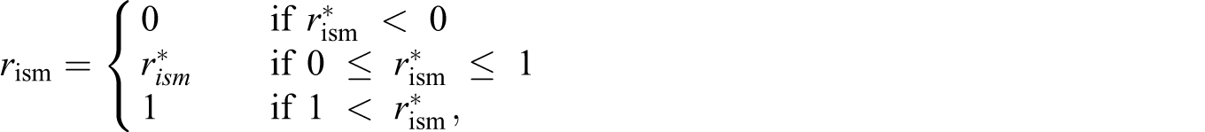
Normalizing U(L) to 0 without loss of generality, we find that there exists a threshold probability, p*:

This threshold depends upon five factors: (i) U(W), the utility of winning the match; (ii) (π H − π), the expected increase in the match-winning probability if the umpire’s call is reversed; (iii) (π − π L ), the expected increase in the match-losing probability if the umpire’s call is challenged but not reversed, and thus the option value of another challenge opportunity is lost; 16 (iv) the disutility from an unsuccessful challenge, c; and (v) the extra utility from a successful challenge, b. Note that (π H − π) and (π − π L ) pertain to one’s overconfidence, which can be defined as the tendency to overestimate the chance of obtaining a favorable outcome—and to underestimate the chance of obtaining an unfavorable outcome—as a result of a presumptuous belief in one’s abilities. 17 In this case, the favorable outcome is winning the match and the unfavorable outcome is losing the match; the ability in which the players presumptuously believe is their ability to make a successful challenge. Thus, an overconfident player will overestimate (π H − π) and underestimate (π − π L ), due to his presumptuous belief in his ability to make a correct challenge.
Except for U(W), which is constant for a player within a match, the remaining four factors (i.e., [π H − π], [π − π L ], b, and c) may vary over the course of the match. They should be evaluated subjectively based on the situations within the match.
Challenge Utilization and Success Rates
In our simple model, the individual player’s decision-making process is summarized simply by the threshold probability. However, one empirical difficulty is that the threshold probability is not observable. Therefore, in our empirical analysis, we will examine two aggregate statistics of challenging behavior that are informative about the threshold probability.
First, we examine the challenge utilization rate per set. Each player is allowed to use as many challenges as possible in each set until they have accumulated two “wrong” challenges (plus a third challenge when the set score is 6-6 and the set reaches a tiebreak). Overall, we observe more challenges from more accurate or luckier players. In order to disentangle a player’s intention to utilize his available challenges from his ability to detect the umpire’s wrong calls (or his luck), we top code the number of challenges to two (or three for a tiebreak set) in each set. Then, we obtain the challenge utilization rate by dividing the top-coded number of challenges by the number of challenge opportunities available in the set. If p* is the threshold probability in the set, then the challenge utilization rate for the set is as follows:

where n denotes the total number of plays within the set in which the umpire’s judgements are against the player, and TB is 1 if there is a tiebreak in the set and 0 otherwise. Note that the utilization rate depends not only on p* but also on n, TB, and f. After removing the effects of n, TB, and f, the remaining variation in the challenge utilization rates across players and matches should be attributable to differences in p*. Furthermore, as can be seen from Equation (2), after accounting for differences in U(W) across players and matches, the variation in p* is attributable to differences in the factors, π, π H , π L , c, and b.
Second, we examine the probability of the player successfully reversing the umpire’s call, that is, the challenge success rate:

The success rate depends upon p* and f(⋅). As with the utilization rate, after accounting for differences in f and U(W) across players and matches, the variation in p* should be attributed to differences in the factors, π, π H , π L , c, and b.
Our empirical analysis in the next section is based on the simple model. The parameter in which we are chiefly interested is the threshold probability, p*, since it can indicate how players assess their winning probabilities as well as the disutility from failure in a challenge and the utility from success. Ideally, we want to compare the thresholds of men and women. That is, we want to test whether E(p*|Male, X) = E(p*|Female, X), where X is the vector of control variables representing players’ characteristics and the contexts in which individual challenges occur. However, it is not possible to identify the threshold per se, and therefore, we choose some observable variables that are expected to influence the threshold. For instance, we hypothesize that a certain variable x affects the threshold probability. Suppose that we estimate the impacts of x on r (utilization rate) and s (success rate), that is,

This result means that we can test gender differences in terms of the impact of x on the threshold. We can infer that there is a gender difference in the threshold if we find that, for example, a variable increases the challenge success rate for women but not for men. Generally, if the signs of the marginal effects differ between men and women, this at least implies that the threshold is determined differently by gender.
In our approach, we are able, not only to examine how x influences the threshold probability but also to check the validity of the model by examining whether
However, one significant limitation of our approach is that that we cannot identify the exact channels through which x affects the threshold probability. For example, an increase in the threshold probability due to a decrease in (π H − π) is observationally equivalent to that due to an increase in c (and likewise, an increase in [π H − π] is observationally equivalent to that due to an increase in b, etc.). Still, we believe that our findings will teach us how individuals make risky choices in competitive environments with extremely high stakes. We will explore possible explanations in the fifth section 5.
Estimation and Data
Estimation Methods
The main empirical implication of our model in the previous section is that we can infer the determinants of the threshold probability from an examination of the determinants of the challenge utilization and success rates. This suggests that we should estimate the equations determining the utilization and success rates.
First, we estimate a Tobit model with two-sided censoring for the challenge utilization rate (corresponding to r in Equation [3]) for each gender, separately.

where the subscripts i, s, and m represent the individual player i, set s, and match m. We interpret
Based on the results from the previous section, we include not only the total number of games played in the set but also the proportion of games won by the opponent in the set. Intuitively, one could imagine the utilization rates in a particular set being positively correlated with the total number of games played in that set. The “relative number of games won by the opponent” variable proxies the number of the umpire’s calls that have not been in favor of the player, n, in Equation (3). The vector Xism includes x’s that we hypothesize will affect the threshold probability: the logarithm of the player’s self-ATP ranking, the logarithm of the opponent’s ATP ranking, 18 a dummy variable that equals 1 if the player won the first set and the current set is the second set, a dummy variable which equals 1 if the player lost the first set and the current set is the second set, a dummy variable that equals 1 if the current set is the third set, and a dummy variable that equals 1 if there is a tiebreak in the current set. In addition, taking 2006 as the base year, 2-year dummies for 2007 and 2008 are included in order to capture any time trend in the utilization of challenges.
Lastly, the variable αim is the player-by-match fixed effect (FE). Recall that we want to infer how a certain variable, representing the player’s or the match’s characteristics, affects p*. However, as can be seen in Equation (2), p* also depends on U(W), which is fixed for a given player in a particular match. We remove this confounding effect by including the player-by-match FE. It is also our key identification assumption for estimating
Note that the player-by-match FE should absorb any umpire-specific effects. Also, the FE should capture any individual-player-specific effects. For the sake of robustness, we tried to include the match- and player-specific FEs separately, but the results were similar.
For the success rate, we use challenge-level data, and estimate the following binary dependent variable model separately for each gender:

where skism indicates whether the kth challenge by individual i in set s of match m is successful. Thus, the expected value of the dependent variable for a player in a match corresponds to s in Equation (4).
As in the case of utilization estimations, the vector of control variables, Zkism, includes the logarithms of both player’s rankings, together with some general characteristics of the set in which the particular challenge was made: a dummy variable that equals 1 if the player won the first set and the current set is the second set, a dummy variable that equals 1 if the player lost the first set and the current set is the second set, and a dummy variable that equals 1 if the current set is the third set. For the most part, the challenge-specific control variables follow the spirit of Abramitzky et al. (2012) and include the values of the following when the challenge was made: total number of games played, proportion of games won by the opponent, a dummy variable indicating whether the point ended naturally or the player stopped during the play, a dummy variable indicating whether the game score was a deuce, a dummy variable indicating whether the game score was 40-0 or 0-40, time elapsed since the start of the match, a dummy variable indicating a tiebreak game, an indicator of whether the shot landed on the opponent’s side of the tennis court, and an indicator of whether the challenge was the second one in the set. 19 In addition, where appropriate, 2-year dummies for 2007 and 2008 are included in order to capture any time trend in the success rates.
Like αim in the utilization rate equation, the variable δ im is the player-by-match FE. As in the utilization rate equation, we interpret the coefficients for the variables in Zkism as the effects of c, π H and π L on the threshold probability, under the assumption that the FE plays a role of controlling for U(W) and f. Due to the presence of the FE, we use an FE Logit model (FE-Logit) to estimate Equation (4), under the assumption that Vkism follows the logistic distribution. Again, we also estimate the random-effect Logit (RE-Logit) models for success rates in terms of robustness checks.
Data and Descriptive Statistics
In March 2006, starting with Miami’s Sony Ericsson Open, the professional men’s and women’s tennis bodies, the ATP and the WTA, decided to give players a chance to challenge some calls by the chair umpires (see Appendix A for more details on the challenge system). We focus mainly on men’s Masters’ and women’s Tier I events, since these tournaments involve both men and women playing matches that are the best (two) out of three sets. 20 Our data set covers all such tournaments in 2006-2008 for which the ATP and WTA had challenge information. Some women’s tournaments, especially those in 2006, did not use the challenge system or keep compiled detailed challenge records; thus, we were not able to include those events in our analysis. As a result, most of the Tier I women’s tournaments in 2006 were not included in our analysis.
The final data set we use includes 331 men’s matches and 149 women’s matches. The data are constructed from the challenge review reports provided directly to the authors by ATP and WTA. Figure 1 presents an example report. We had to drop some tournaments because some crucial variables, such as scores, had not been recorded in the relevant reports. We also dropped four matches from which players retired, so that the matches were not completed.
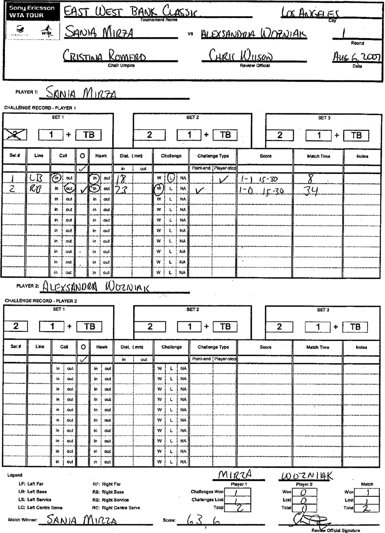
Example challenge report.
Table 1 presents summary statistics of some match characteristics. Overall, it seems that men’s and women’s matches are comparable. However, we find that men’s matches are slightly more competitive than those of women. Men’s matches are more likely to go to the third and deciding set, more likely to be an upset, and tend to have more tiebreaks. Also, the probability of winning the match conditional on winning the first set is slightly lower for men. 21
Match and Challenge Characteristics.
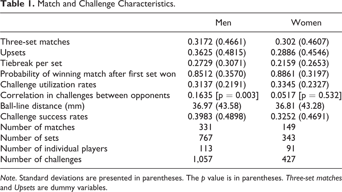
Note. Standard deviations are presented in parentheses. The p value is in parentheses. Three-set matches and Upsets are dummy variables.
Another interesting difference is found in the correlation between the numbers of challenges between two players. The correlation is significantly positive in men’s matches (0.16), while it is smaller and statistically insignificant in women’s matches (0.05). Two players’ challenges may be correlated because they are judged by the same umpire. However, if this were the case, there would be no reason why the correlation would only exist for men. One possible explanation of the gender difference is that, for male players, challenges are sometimes a response to the opponent’s challenges. 22
For both men and women, the average number of challenges per set is significantly less than two: 0.31 for men and 0.33 for women. That is, neither male nor female players utilized all available challenges in a set fully. 23 This is somewhat surprising, since the opportunity cost of using a challenge drops considerably as a set approaches its end, finally becoming virtually zero at the last play that ends the set. Thus, low utilization rates suggest that there is a stigma associated with a wrong or unnecessary challenge, and/or that there is a strong incentive to save a challenge for a critical moment, which is likely to occur at the end of a set. 24
The average success rate of challenges is somewhat higher for men: men’s success rate is about 40% while women’s is about 33%, but they are not statistically different. The average ball-line distance is similar for both genders, about 37 mm.
Estimation Results
Challenge Utilization and Success Rates
We present the utilization rate estimation results in Table 2. We estimate the determinants of the utilization rates of male and female players separately using both the RE and FE approaches. For each approach, we also estimated the utilization rate equation using the pooled sample of male and female players with all explanatory variables interacted with the gender dummy, in terms of estimating the coefficient differences across genders and their standard errors. These differences and corresponding standard errors for the RE and FE methods are presented in columns 3 and 6, respectively. The success rate estimation results are presented in Table 3 in a similar fashion.
Challenge Utilization by Gender.
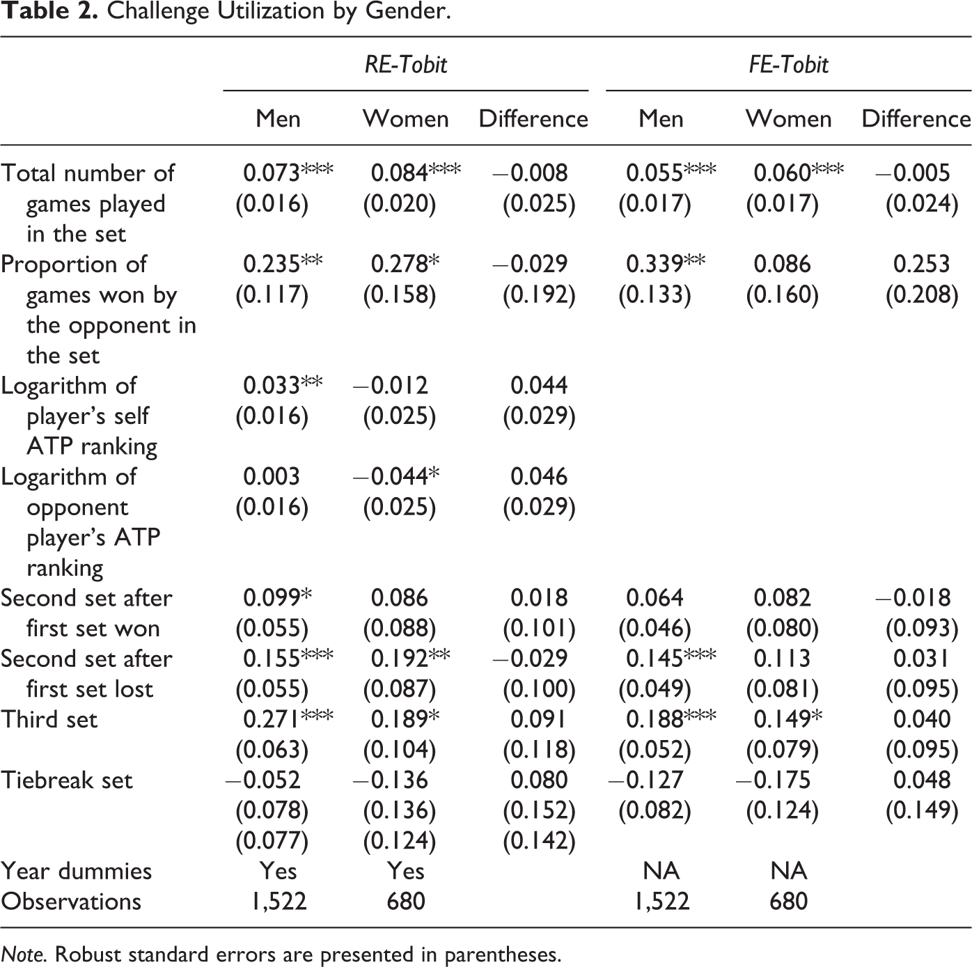
Note. Robust standard errors are presented in parentheses.
Success Rates by Gender.
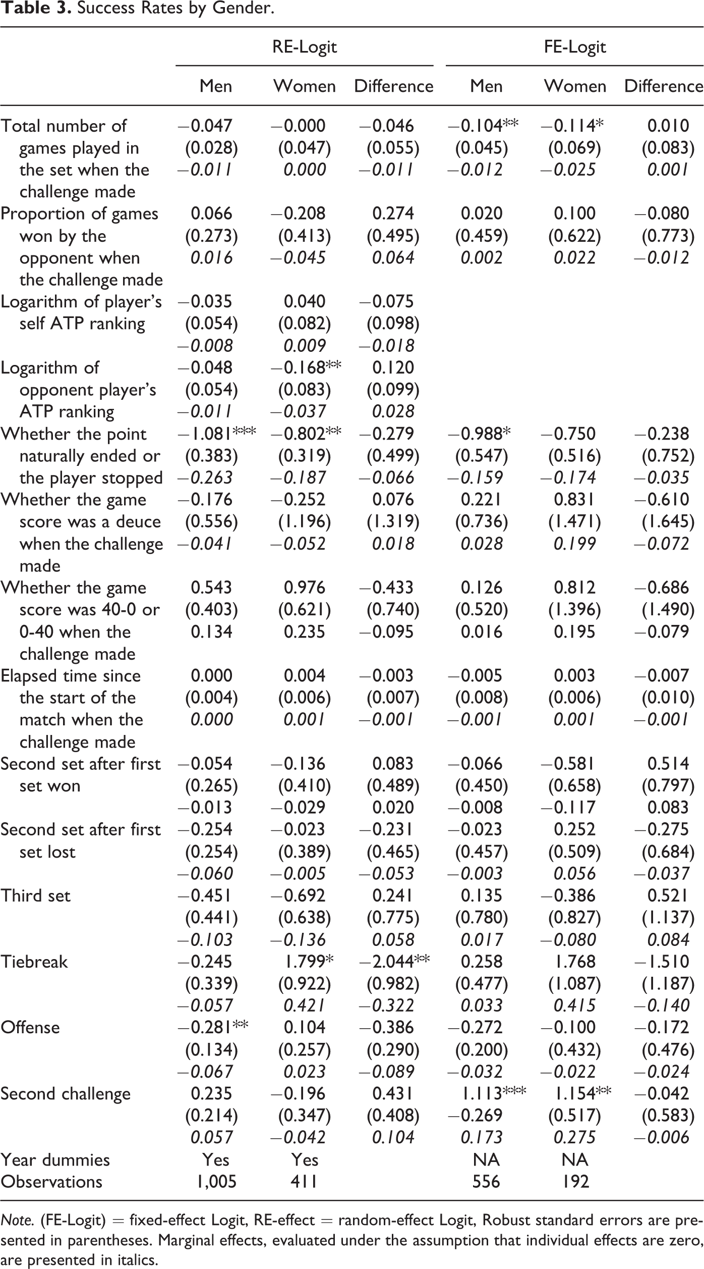
Note. (FE-Logit) = fixed-effect Logit, RE-effect = random-effect Logit, Robust standard errors are presented in parentheses. Marginal effects, evaluated under the assumption that individual effects are zero, are presented in italics.
Overall, the results seem to support the validity of our model, where an individual challenging decision is described as a threshold strategy. We find that when the challenge utilization rate is higher, the success rate tends to be lower, and vice versa. Although there are a few exceptions, the sign of
The results regarding the utilization rate in columns 1 and 2 of Table 2 are quite similar for male and female players. First, as the number of total games played in a set increases, challenge utilization rates increase significantly for both genders in both the RE and FE models. However, this robust positive correlation is clearly intuitive and not surprising: the larger the number of games played, the greater the chance of a player challenging an umpire call. The results also indicate that, keeping all else constant, particularly the total number of games played, a player tends to use more challenges as the opponent wins relatively more games in a set. Again, this association is not surprising if we consider the variable as a proxy for the number of unfavorable judgements. Equation (3) showed that, the more judgements there are against a player, the more likely the player is to challenge. Nevertheless, this finding is more robust for male players than for females, because the estimated coefficient is significant in both the RE and FE models for males, while it is only significant in the RE model for females. Utilization rates are also significantly higher in the second and third sets than in the first set. 25 More specifically, it turns out that a player who has lost the first set will tend to use more challenges in the second set. This effect is significant for men in both the RE and FE models, and for women in the RE model. This is in contrast to when the player has won the first set, in which case there is no significant change in the utilization rate of the second set, except for the RE model of male players. Regardless of their gender, all players challenge more during the third and deciding set. These relationships are robust in both the FE and RE models, though they seem stronger for male players. In addition, RE estimations suggest that, while a higher self-ranking tends to increase male utilization rates significantly, female utilization rates decrease significantly as the opponent player’s ranking increases.
As was mentioned previously, columns 3 and 6 of Table 2 represent the coefficient differences between male and female players and the standard errors of those differences for RE and FE models, respectively. Given the similarities between male and female challenging strategies, as suggested by separate estimation results, it is not surprising that the coefficient differences for all variables turn out to be statistically insignificant in both the RE and FE estimation results. This exercise also confirms the similarity of the challenging behaviors of male and female players in a statistical sense.
Next, we turn our attention to the success rate results presented in Table 3. Note that our set of explanatory variables is richer in the success rate estimations, as we are able to control for challenge-specific variables by using individual challenge data. The findings indicate that a challenge made closer to the end of a set is less likely to be successful. This is suggested by the negative coefficient estimated on the total number of games played in the set up to the time of the challenge. The coefficients are significant for both male and female players in the FE model but turn out to be insignificant in the RE one, although they have the same negative sign. Looking at columns 3 and 6, however, suggests that there is not a statistically significant gender difference with respect to this correlation between the total number of games played at the time of a challenge and its success probability. We also notice from Table 3 that a female player is more likely to make an unsuccessful challenge when the opponent has a relatively higher ranking, but we do not observe any such significant relationship for male games. Another factor that seems to be important in explaining challenge success rates is the type of challenge; that is, whether the challenge point ended naturally or the player stopped during the play turns out to be significant, particularly for males’ success rates. A player’s challenge is more likely to be unsuccessful when the point ends naturally than when the player stopped. Again, the gender difference with respect to this factor is not significant in either the RE or FE models. In terms of success rate results, the major difference between males and females appears in the case of a tiebreak. At tiebreaks, females are more likely to make a correct challenge, while males are more likely to make an incorrect challenge, and this gender difference is statistically significant. The results are similar in the case of a challenge made in an offense, but the difference is less significant. These findings are particularly noticeable in the RE model. The FE model still suggests the same conclusions in terms of their direction, but they are less apparent in a statistical sense. Finally, a second challenge is more likely to be successful than the first challenge for both male and female players, especially in the FE models. This makes sense intuitively, as a player would be expected to be more careful in utilizing his second challenge if it were potentially his last.
Embarrassing Challenges
In this subsection, we focus on somewhat extreme challenges. If a challenge is wrong by more than 50 mm, we call it an “embarrassing challenge” here. 26 Figure 2 is the histogram of ball-line distances. For wrong challenges, the distances are given a negative sign. It is quite surprising that some wrong challenges were made when the distance was quite long, for example, more than 200 mm. In fact, it seems that wrong challenges have larger distances. The histogram looks asymmetric and slightly skewed to the left, as more than 60% of the overall challenges are unsuccessful. This suggests that, although many of the embarrassing challenges are simply players’ unintentional mistakes, some players may be exploiting challenges strategically. Comparing the frequencies of making such bad calls by gender would be interesting for the purpose of our article. Certainly a player is more likely to make such a challenge when he or she is far away from the ball. However, it is also possible that players may make such bad calls deliberately, in spite of the fact that the success rate is low, in order to slow down the opponent’s momentum or to obtain rest. 27 Either way, these challenges may involve some strategic behavior in terms of increasing match winning probabilities. Finally, embarrassing challenges might be a consequence of emotional reactions to some intensively competitive high-stake moments.
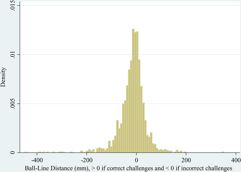
Ball-line distance.
A descriptive look at the data suggests that men and women have the same ratio of embarrassing challenges: of each gender’s challenges, 17% are embarrassing challenges. 28 However, in tiebreaks, that is, when the set is at stake, men make many more of them (34%), while women make many fewer of them (9%). Men also tend to make more embarrassing challenges when the ball lands on the other side of the net, that is, when it is rather risky to challenge since the player’s view is impeded.
The estimation results for embarrassing challenges are presented in Table 4. Consistent with the descriptive statistics, when controlling for other factors in a regression setting, men are still a lot more likely to make embarrassing line-call challenges at tiebreaks and offenses than women. Moreover, the gender differences in regard to these variables turn out to be statistically significant, particularly in RE estimations. From Table 4, we also note that a higher ranked male player is more likely to make an embarrassing challenge, while a higher ranked female is less likely to make an embarrassing challenge. This gender difference in challenging behavior is again statistically significant. Finally, while the propensity to make an embarrassing challenge increases with the opponent’s ranking in male games, we do not observe such a statistically significant correlation in female games. This finding also supports the previously mentioned idea that men’s line-call challenges are more likely to be provoked by their opponents.
Embarrassing Challenges.
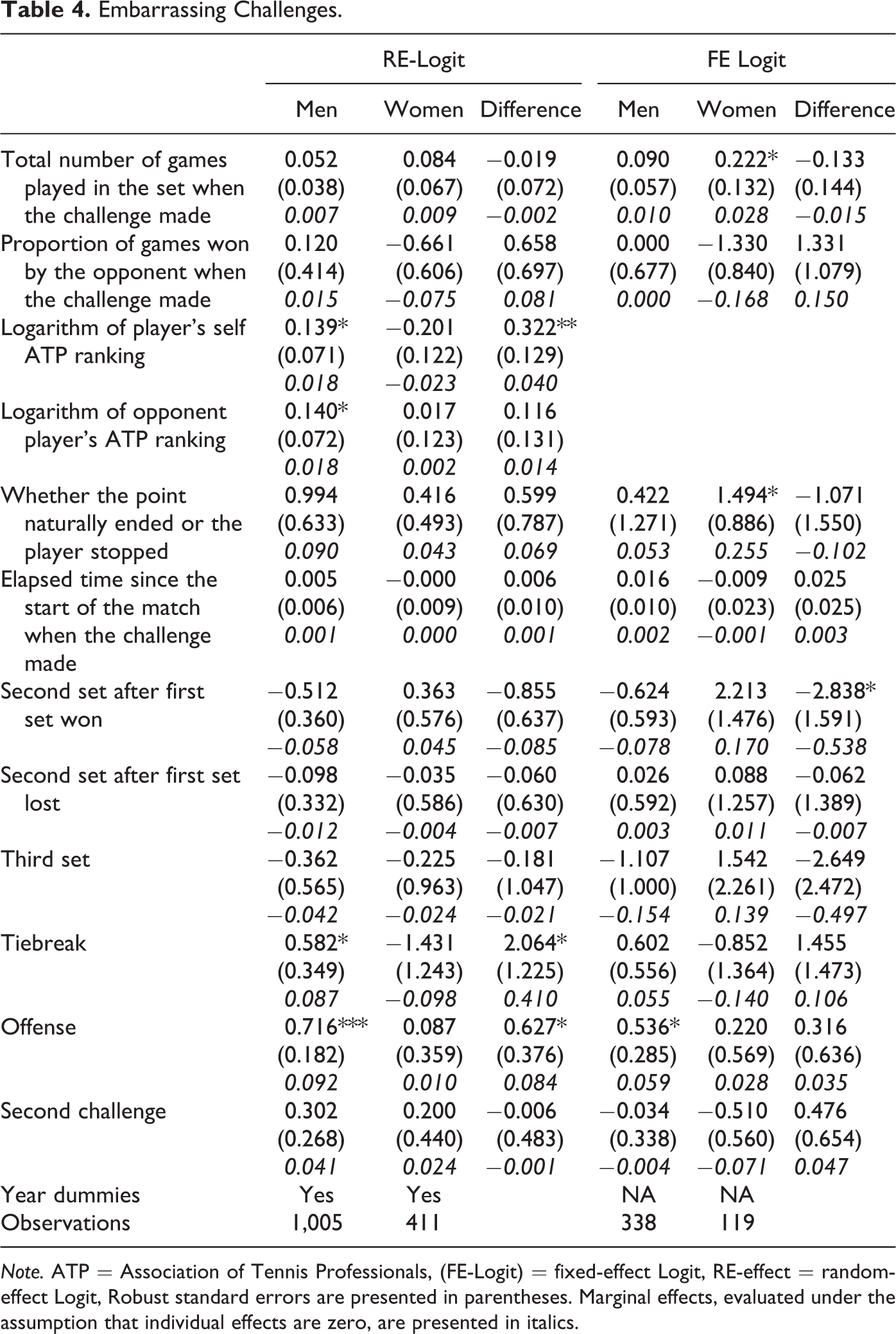
Note. ATP = Association of Tennis Professionals, (FE-Logit) = fixed-effect Logit, RE-effect = random-effect Logit, Robust standard errors are presented in parentheses. Marginal effects, evaluated under the assumption that individual effects are zero, are presented in italics.
Interpretations of Gender Differences
Our empirical analysis mentioned previously provides some evidence in support of our simple model that describes players’ challenges as choices made according to a threshold probability. As we mentioned earlier, these choices involve a risk-taking behavior, because each player has a limited number of challenge rights in a given set. As one can imagine, it might be crucial to save some of these challenges for the most critical points, in terms of maximizing individuals’ match winning probabilities. Thus, when deciding to make a challenge, a player must weigh the risks involved and choose the best timing to utilize these limited number of opportunities.
The results indicate that male and female players exhibit many similarities in their use of line-call challenges, which is not surprising, since they are all top-notch professionals and play high-stake games. Still, we do find that challenge decisions are made somewhat differently by male and female players. Recall that, in our model, the threshold probability is determined by factors parameterized by b, c, (π H − π), and (π − π L ). In this section, we will explore possible interpretations of our findings about gender differences within the framework of our optimal decision making model.
Croson and Gneezy (2009) list three potential explanations for gender differences in any decision making that involves risk taking: (1) “emotions,” (2) “overconfidence,” and (3) “perception of risk.” Clearly, in our framework, b and c pertain directly to “emotions,” via pride and shame, and partially to “perception of risk.” In addition, (π H − π) and (π − π L ) pertain to “overconfidence” directly, and to “perception of risk” to some extent.
We have already noted that an overconfident player would overestimate (π H − π) and underestimate (π − π L ) when making a challenge decision, due to his presumptuous belief in his tennis playing ability. Previous studies on overconfidence have consistently shown that individuals overestimate the precision of their knowledge (Alpert & Raiffa, 1982). In addition, overconfidence tends to be more severe for difficult tasks (Fischhoff et al., 1977). Even our world-class professional players can be subject to a cognitive bias due to overconfidence. Based on a sample of about 3,000 entrepreneurs, Cooper, Woo, and Dunkelberg (1988) found significant levels of overconfidence in these entrepreneurs’ self-perceptions of their business abilities. About 81% of them perceived their own likelihood of success with these abilities to be at least 70%, while a third viewed their odds of success as 100%. Meanwhile, they had much less favorable outlooks on other businesses that were comparable to theirs. 29
Various psychological studies have found that men tend to be more overconfident than women (e.g., Beyer, 1990; Beyer & Bowden, 1997; Lichtenstein et al., 1982). 30 According to Niederle and Vesterlund (2007, p. 1087), “while 75% of the men think they are best in their group of four, only 43% of the women hold this belief.”
These factors might potentially help explain the gender differences that we observe in this article. It is interesting to note that the gender differences among professional players are salient mainly at competitively intense high-stakes moments. We observe the two most notable gender differences during tiebreaks. First, the results on the success rate for female players are opposite to those for male players. The success rate is lower than usual for men in tiebreaks, whereas it is higher than usual for women, despite very similar utilization rates by the genders. Second, in tiebreaks, men make more embarrassing challenges than usual and women make fewer embarrassing challenges than usual (in spite of the fact that the two genders have equal ratios of embarrassing challenges to all challenges). In both cases, the gender differences are statistically significant.
One possible explanation for both of these stark gender differences in tiebreaks could be that women play more conservatively at such times. That is, women may become relatively more risk averse than men in intensely competitive high-stake moments. This is consistent with the finding of Paserman (2010) that the odds of making an unforced error relative to hitting a winner at crucial junctures of the match fall for women, while they remain constant for men. 31
Another potential explanation for the significant gender differences in tiebreaks could be that the overconfidence of male players leads them to make more risky challenges, while the lower level of overconfidence of female players leads them to make fewer risky and embarrassing challenges in similar situations. 32
Our theoretical approach assumes that, in part, players with a lower c will feel much less shame for a bad challenge, and players with a higher b will feel much more pride for a good challenge. However, what about the observed differences in challenging behaviors between men and women in relation to these parameters? Are there any potential differences between men and women with respect to their level of concern over making a mistake or their fear of experiencing shame?
There is some evidence that women tend to take negative feedback more seriously than men (see for instance Roberts & Nolen-Hoeksema, 1989). Second, due to their more emotional nature, women may view a negative signal as an indicator of their self-worth, rather than simply of their onetime performance on a task. Dweck (2000) suggests that women may fall into “confidence traps” more easily than men. In addition, Brizendine (2006) reports that girls’ well-developed brain circuits (for gathering meaning from faces and responding to unspoken cues in others) push them to comprehend the social approval of others very early. These findings of the differences between genders also seem useful in providing potential explanations of why women might take a more conservative approach in their playing strategy in tiebreaks and make fewer embarrassing challenges than men.
The fact that the challenge utilization rate is very low for both genders implies that all tennis players have concerns about making unsuccessful challenges. Otherwise, all of the remaining challenges of every player could easily be used as strategic ploys to at least change the momentum of the game by irritating the opponent or to obtain a breather for the player who challenges the call, whenever possible. This is hardly the case for female players and is only the case for male players when a lot is at stake in the match, such as during tiebreaks, which suggests that the extent of such concerns differs for men and women.
At high-stake moments in a match, such as tiebreaks, the embarrassment of a strategic challenge (i.e., a challenge with virtually no chance of success) may be overcome by its strategic benefits, such as stalling the opponent’s momentum and getting a breather. In addition, such a strategic advantage may even have a signaling value, with the challenging player’s signal being, “I’ll keep fighting at all costs until the last point of the match and won’t allow any easy victory, without caring much about shame and embarrassment.” Our gender difference findings indicate that a male player is relatively more likely to send such a strategic signal. A player who sends such a signal of resilience may hope to deter both current and future opponents to some extent and, as such, to gain a mental edge over them, however small. 33 Our finding of male player’s challenges being more likely to be provoked by those of their opponents can be considered along these lines as well.
Nevertheless, no kind of strategic ploy is carried out by all players at all times. Evidently, even the most strategic players who play such mind games must resort to such strategic ploys only when it is worth it, namely when they have a chance to turn things around, such as in tiebreaks.
Although we do not discuss them in detail here, similar explanations might apply to the additional significant gender differences observed in our empirical analysis mentioned previously.
Conclusion
Tennis line-call challenges provide a suitable context in which to investigate the origins of gender differences in a competitive setting with large monetary rewards. Given the nature and design of the tennis market, gender discrimination in terms of pay or participation rates on the demand side are unlikely to happen. This makes professional tennis an attractive setting for investigating whether men and women respond differently to competitive pressures. Unlike in an experimental setting, the prize money gained by winning matches is reasonably large. Thus, by examining the behavior of individuals in such a real setting, we aim to make a significant contribution to the existing literature on gender differences.
To summarize our results, we observe that the genders are very similar in terms of their line-call challenge utilization rates. Specifically, the utilization rates of both male and female players are significantly higher the higher the total number of games played in the set and increase significantly with the proportion of games won by the opponent. Intuitively, utilization rates are also significantly higher in the second and third sets than in the first set. While a higher self-ranking tends to increase male utilization rates significantly, female utilization rates decrease significantly as the opposing player’s ranking increases. Nevertheless, all of these gender differences in utilization rates turn out to be statistically insignificant.
In terms of success rates, the major differences between males and females appear in challenges made in tiebreaks. In tiebreaks, females are more likely to make correct challenges, while males are more likely to make an incorrect challenges, and this gender difference is statistically significant. The results are also similar in the case of a challenge made in an offense, but the difference is less significant.
Furthermore, men are a lot more likely to make “embarrassing” line-call challenges in tiebreaks and offenses than women. Although a higher ranked male player is more likely to make an embarrassing challenge, a higher ranked female is less likely to do so. Finally, the propensity to make an embarrassing challenge increases with the opponent’s ranking in male games, but we do not observe any such statistically significant correlation in female games. When coupled with the descriptive statistics of the data, this finding might suggest that men’s line-call challenges are more likely to be provoked by their opponents.
The major gender differences found at crucial moments of the match, such as tiebreaks, suggest that male players try to win at all costs, while female players accept losing more gracefully. In that sense, this finding extends the Niederle–Vesterlund finding to a domain in which neither men nor women are choosing to shy away from competition: Even if it involves very high stakes, women are less likely to try to win the competition at all costs than men. Differences in factors such as risk aversion, overconfidence, pride, shame, and strategic-signaling behavior are some of the potential explanations of our main gender-difference findings in line-call challenges.
Finally, our article studies the risk-taking decisions of two highly skilled professionals in a high-stakes “interactive environment,” in which their risk-taking trajectories are shaped by the constantly changing score and momentum of the match. In addition, these professionals make their decisions “in front of others.” We are not aware of any previous study that has looked at risk taking in an “interactive environment” and “in front of others.” The limited literature on other topics where the audience is a factor, such as the study by Charness and Rustichini (2011), suggests that people do not always behave in the way that would be expected when faced with an audience. Given that many individuals do not make their risk-taking decisions in isolation or seclusion, further research into risk-taking behaviors in “interactive environments” and “in front of others” will be significant and fruitful.
Footnotes
Appendix
Acknowledgment
We would like to thank the officials from both ATP and WTA who generously shared their confidential challenge data with us, and Chris Doucouliagos, Nick Feltovich, Jinyoung Kim, and the participants of various conferences and seminar presentations for their many comments and suggestions.
Declaration of Conflicting Interests
The authors declared no potential conflicts of interest with respect to the research, authorship, and/or publication of this article.
Funding
The authors disclosed receipt of the following financial support for the research, authorship, and/or publication of this article: This research is supported by Ministry of Culture, Sports and Tourism (MCST) and Korea Culture & Tourism Institute (KCTI) Research & Development Program 2012. Lee’s work was supported by the Sogang University Research Grant of 2013 (201310065.01).