Rank-Based Groupings and Decision Making

Abstract

Rank-based groupings are uninformative signals of quality when the exact rank is known; therefore, they should be ignored in decision making. However, evidence is presented that rank-based groupings are used to determine the compensation of rookie players in the National Football League (NFL). The NFL draft, which largely determines rookie compensation, provides two signals of player quality, selection number, and round. However, the rounds are simply groupings based on selection number; thus, the rounds should not affect subsequent decisions. Sharp regression discontinuity design (RDD) estimates of discontinuities in rookie compensation at the round cutoffs are shown to be very large and robust. The first to second round discontinuity is −US$240,000 to −US$250,000, or 36% of the average salary of the first selection in the second round. The second to third round discontinuity is −US$60,000 to −US$70,000, or 17% of the average salary of the first selection in the third round. The results show rookie compensation, which comprises a large share of career earnings, is subject to heuristic thinking.

Keywords

rank-based groupings regression discontinuity compensation NFL NFL draft

Introduction

Often when making decisions people consider rankings as a signal of quality. For example, Salganik, Dodds, and Watts (2006) show how rankings affect behavior in experimental music download markets. However, many times we are presented with not only rankings but rank-based groupings. For example, we see the top 10 songs, books, movies, or college football teams. Such groupings are only informative signals in the absence of the underlying or rank. All information contained in the grouping is provided by the specific rank, which also provides more information.

A simple example of college football rankings helps to illustrate the situation. During the season, college football teams are ranked according to quality. It is very common for people to discuss the top 10 teams. In this case, the grouping is being in the top 10. The underlying characteristic is a team’s exact rank. It is clear if the exact rank is unknown, the grouping is informative about the quality of the team. However, if the ranking is known, the grouping is an uninformative signal.

Similarly, the National Football League (NFL) draft, which consists of seven rounds of selections, provides two signals of expected productivity, selection number, and round. However, several studies have shown draft information to be very noisy signals for productivity (Berri & Simmons, 2011; Hendricks, DeBrock, & Koenker, 2003). Regardless of the noisiness of selection number and round, the round signal is dominated by selection number. Rounds are simply groupings of players based on selection number. Therefore, the rounds are uninformative signals of player quality, given the selection number is known. Since there are 32 NFL teams and each team has the right to one selection per round, we automatically know that selection numbers 1 through 32 are in the first round and selections 33 through 64 are in the second round.¹

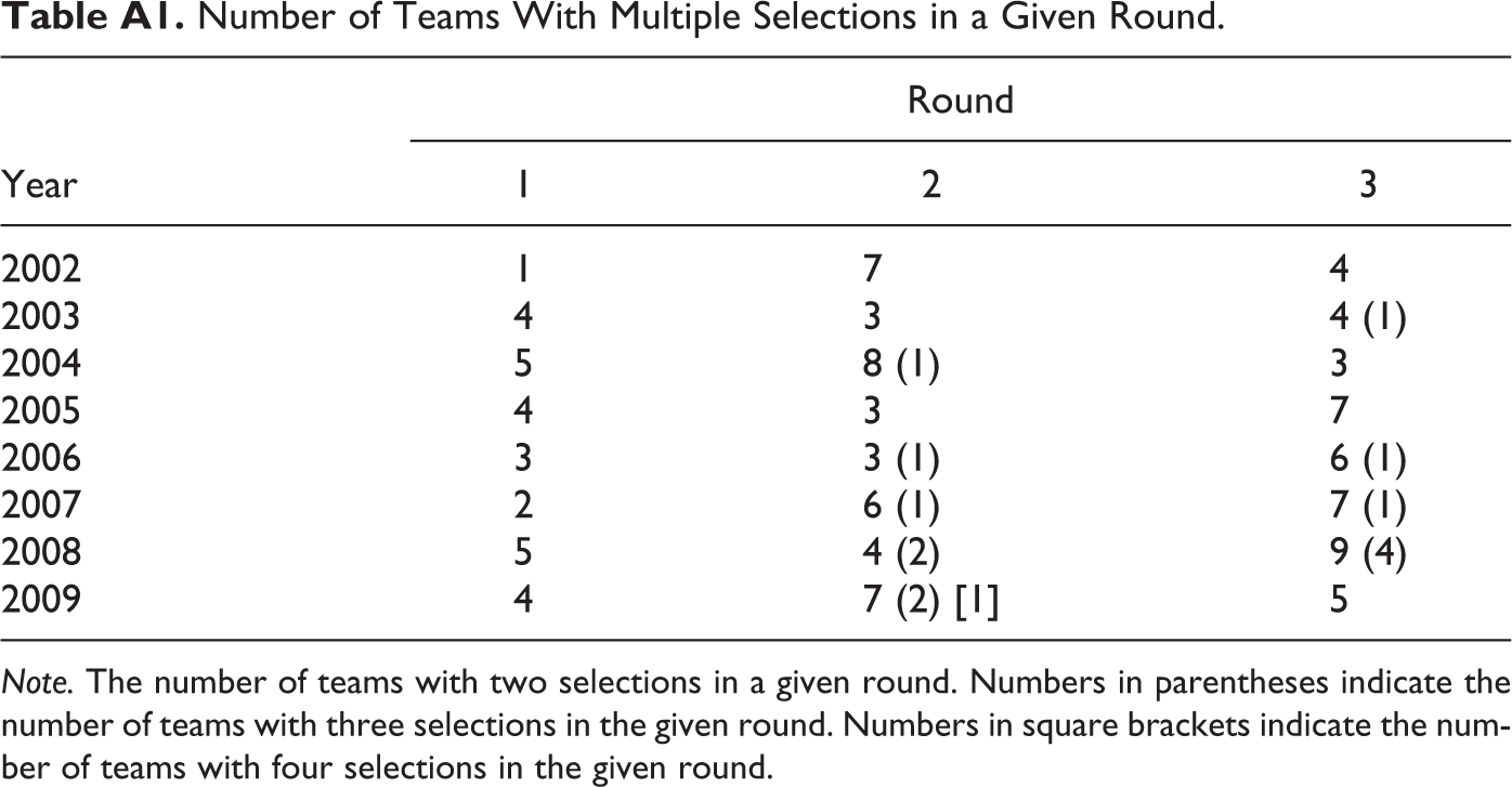
If all teams exercised their rights in each round, the round number would indicate a player’s within-team selection number. However, teams use their selections as assets that can be traded for other selections in the same year, selections in future years, or to obtain nonrookie players. As a result, it is very common for teams to select multiple times in a given round and for teams to not select a player in a given round (see Appendix for the number of teams with multiple selections in a given round).

As the rounds are simply groupings based on selection number, they should be ignored in decision making. However, we present evidence that in the presence of the noisy draft signals the NFL rookie labor market relies on heuristic thinking.² The rounds are very influential in the evaluation of expected productivity for rookies. Players are even referred to by the media, or members of a franchise, as first round or second round picks. The heuristic thinking manifests itself as discontinuities in the compensation of drafted NFL rookies precisely and uniquely at the round cutoffs. Discontinuities in compensation are very important because initial compensation has a large impact on the total career earnings of NFL players. As the average NFL career is very short, rookie compensation comprises a large portion of career earnings.

Model

A player’s compensation, w, is dependent on his expected productivity. When the compensation of rookies is determined, productivity is unknown, since these players have not participated in any NFL games or practices.

w_{n} = W [E (θ_{n}), X_{n}] .

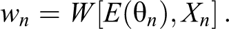
Where n indexes players, θ is the random variable for a player’s productivity, and X is the vector other factors determining compensation.

Teams use selection number, S, and round, R, as signals of expected productivity.

w_{n} = W [E (θ_{n} | S_{n}, R_{n}), X_{n}] .

However, since the round is simply a rank-based grouping of selection numbers we have.

E (θ | S, R) = E (θ | S),

w_{n} = W [E (θ_{n} | S_{n}, R_{n}), X_{n}] = W [E (θ_{n} | S_{n}), X_{n}] .

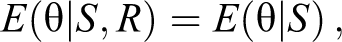
Thus, the round signal should have no impact on rookie compensation. Evidence that the rounds are a significant determinant of rookie compensation suggests the use of heuristic decision making in the market for drafted rookies.³

Sharp Regression Discontinuity Design (RDD) Method

We exploit the structure of the NFL draft to conduct a sharp RDD for the first 3 rounds. The presence of compensatory picks, designed to compensate teams who lost many players to free agency, causes there not to be consistent cutoffs between later rounds (Karimian, 2011).⁴ A sharp RDD requires a cutoff in the data at which point observations move, discretely, from untreated to treated. Let R_i be a binary variable for players selected in the ith round, where i = 1, 2,…,7, and all other variables retain their previously mentioned meanings. If S < c_i , then R_i = 0, and if c_i ≤ S < c_i+1 , then R_i = 1, where c_i is the cutoff point between rounds i − 1 and i. For example, if we examine the effect between the first and second rounds R ₂ is a binary variable for second round selections and c ₂ is selection number 33.

To estimate the size of the round discontinuities, we first estimate a pooled regression using third order polynomials of selection number (Lee & Lemieux, 2010).

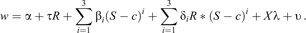
w = α + τ R + \sum_{i = 1}^{3} β_{i} (S - c)^{i} + \sum_{i = 1}^{3} δ_{i} R * (S - c)^{i} + X λ + υ .

The coefficient, τ, on the binary round variable is the average treatment effect (ATE) and X is a vector control variables including year, team, and position fixed effects. By including the interaction terms, R*(S − c), we allow for the effect of selection number to be different between the rounds.

The drawback to the pooled regression approach is that it weighs all observations equally in the calculation of the ATE. Therefore, we estimate the local average treatment effect (LATE) with local linear regression, which minimizes bias (Fan & Gijbels, 1996; Imbens & Lemieux, 2008; Lee & Lemieux, 2010). We use the triangle kernel because it is the optimal weighting function for boundary cases, which directly applies to RDD (Cheng, Fan, & Marron, 1997).⁵ Also, we use the method proposed by Imbens and Kalyanaraman (2012) of calculating the optimal bandwidth.⁶ The method is completely data dependent and derived specifically for RDD to minimize root mean squared error.⁷ Since the selection of bandwidth can have a large impact on results, we use the method proposed by Nichols (2007) and report results for the optimal bandwidth, half the optimal bandwidth, and double the optimal bandwidth.

RDD requires the inability of individuals to perfectly manipulate assignment, called exchangeability, which allows treatment around the cutoffs to be randomized (Lee, 2008; Lee & Lemieux, 2010; Nichols, 2007). This condition is satisfied since prospective rookies cannot be perfectly manipulated into one round or another. The standard tests for manipulation are to examine the density and individual characteristics near the cutoff. In the NFL draft, there is a single player chosen at a given selection number creating equal densities on either side of the cutoff. We present further justification of the exchangeability condition in the Results section.

However, due to the structure of the NFL draft, there are two concerns. First, the average within-team selection number changes between rounds. As previously mentioned, NFL teams trade selections so the change is not discrete, but the average within-team selection number does change. Since selection order within each round, before trades are considered, is the reverse order of previous season team success, team quality is also a concern. Again, due to trades the change is not discrete, but the average team success varies between rounds. As a result, we conduct various robustness checks for these issues, which are further detailed in the Results section.

Data

The data cover every player drafted in the first three rounds of the NFL draft from 2002 to 2009. The data begin in 2002 because the NFL expanded in 2002 from 31 to 32 teams. The data end in 2009, as it was the final year of the collective bargaining agreement (CBA) between the NFL owners and the National Football League Players Association (NFLPA; National Football League, 2008). The CBA originated in 1993, but 2009 was the final year under these guidelines. As compensation in the NFL is dictated by a salary cap, which is specified in the CBA, the data end in 2009 for consistency.

The NFL also has a salary cap for rookies, a cap within a cap. Prior to the draft, the NFL uses a secret formula to determine each team’s specific dollar amount available to sign rookie players. The equation is kept very private to the NFL and is not disclosed to teams, players, players’ agents, or the public (Mirabile, 2007). The NFL makes no attempt, as stated in the CBA, to suggest or restrict how the money is allocated (Florio, 2011). Teams are simply told the amount of money they have to sign their rookie players. A player’s salary cap value is the sum of his base salary, incentive bonuses, and signing bonus prorated for the life of the contract. Due to the amortization of signing bonuses, we use salary cap value as the measure of rookie compensation.

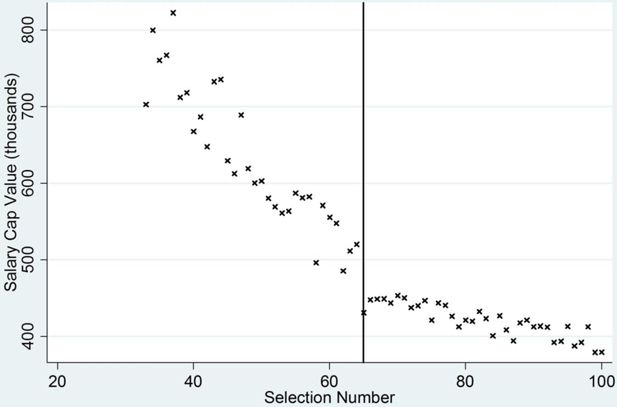
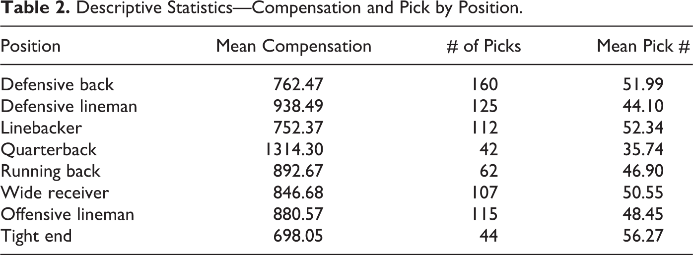
The data were collected from two sources. The USA Today (2011) maintains a database of professional athletes’ salaries. We use drafted rookie salary cap values between 2002 and 2009. The second source, Pro Football Reference (2011), was used to collect all draft and team-related information: selection number, round, year, position, team, and previous season team wins. Descriptive statistics are reported in Tables 1 and 2.

Table 1.

Descriptive Statistics—Mean Compensation by Round and Year.

Variable = Salary Cap Value/1,000
Round	Total	2002	2003	2004	2005	2006	2007	2008	2009
1st	1,521.2	1,335.7	1,334.7	1,425.9	1,546.3	1,500.3	1,532.6	1,773.4	1,723.0
2nd	632.12	555.09	572.14	575.86	610.99	606.82	604.51	848.11	685.87
3rd	423.39	367.78	379.13	375.26	394.68	439.38	451.23	497.76	497.76

Table 2.

Descriptive Statistics—Compensation and Pick by Position.

Position	Mean Compensation	# of Picks	Mean Pick #
Defensive back	762.47	160	51.99
Defensive lineman	938.49	125	44.10
Linebacker	752.37	112	52.34
Quarterback	1314.30	42	35.74
Running back	892.67	62	46.90
Wide receiver	846.68	107	50.55
Offensive lineman	880.57	115	48.45
Tight end	698.05	44	56.27

Results

We first examine the exchangeability condition by analyzing the number of games started in a player’s third season and Pro Bowl selections for players selected near the cutoff between the first and second rounds. We use games started and Pro Bowl selections as productivity measures due to the presence of multiple positions. We calculate both measures for selections 30 through 32 and 33 through 35. The average number of games started for the first round players is 9.96 with a standard deviation of 6.12. For the second round players, the average number of games started in their third season is 10.25 with a standard deviation of 6.12. For the specified first round selections, there are two players who have been selected to the Pro Bowl, through the 2012 season. The total number of Pro Bowls for the first round players is 9. Three second round players were selected to the Pro Bowl, totaling eight selections. Both measures point to the fact that players selected close to the Round 1 cutoff are equal in productivity.

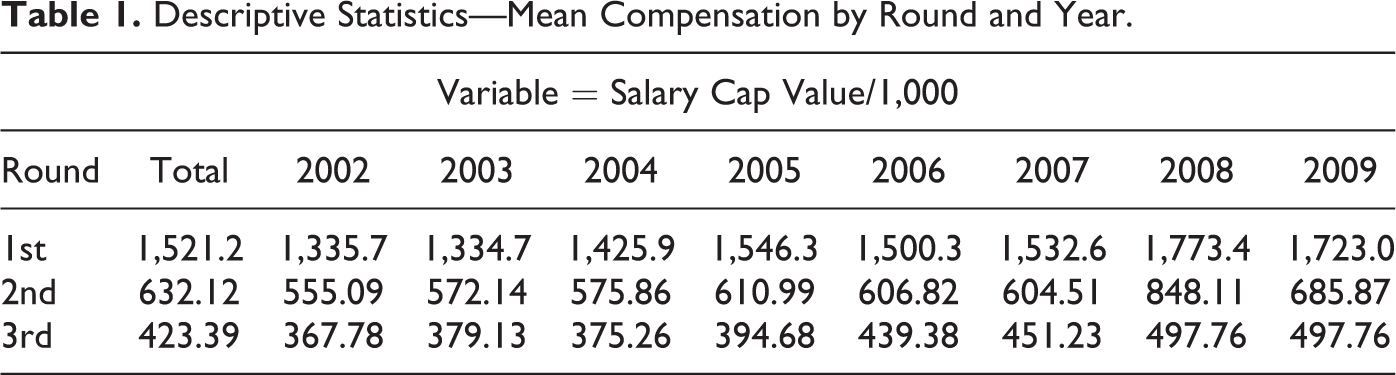
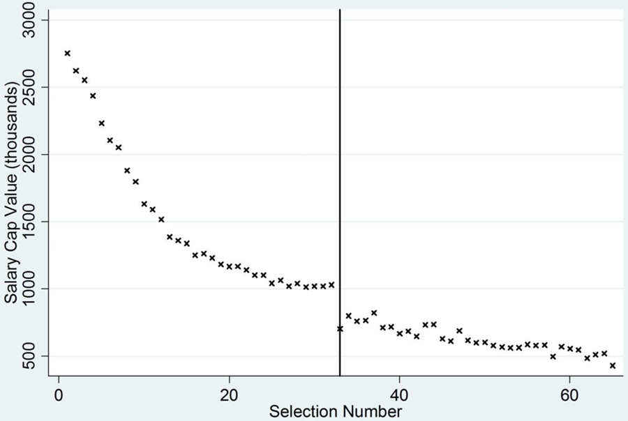
One benefit of RDD is the discontinuity is easily seen on a graph. Figures 1 and 2 display the mean compensation by selection number for the first two rounds and the second and third rounds, respectively.⁸ It is evident that there are indeed discontinuities in salary cap value between rounds.

Figure 1.

First and second rounds mean compensation by selection.

Figure 2.

Second and third rounds mean compensation by selection.

Cubic Regression Results

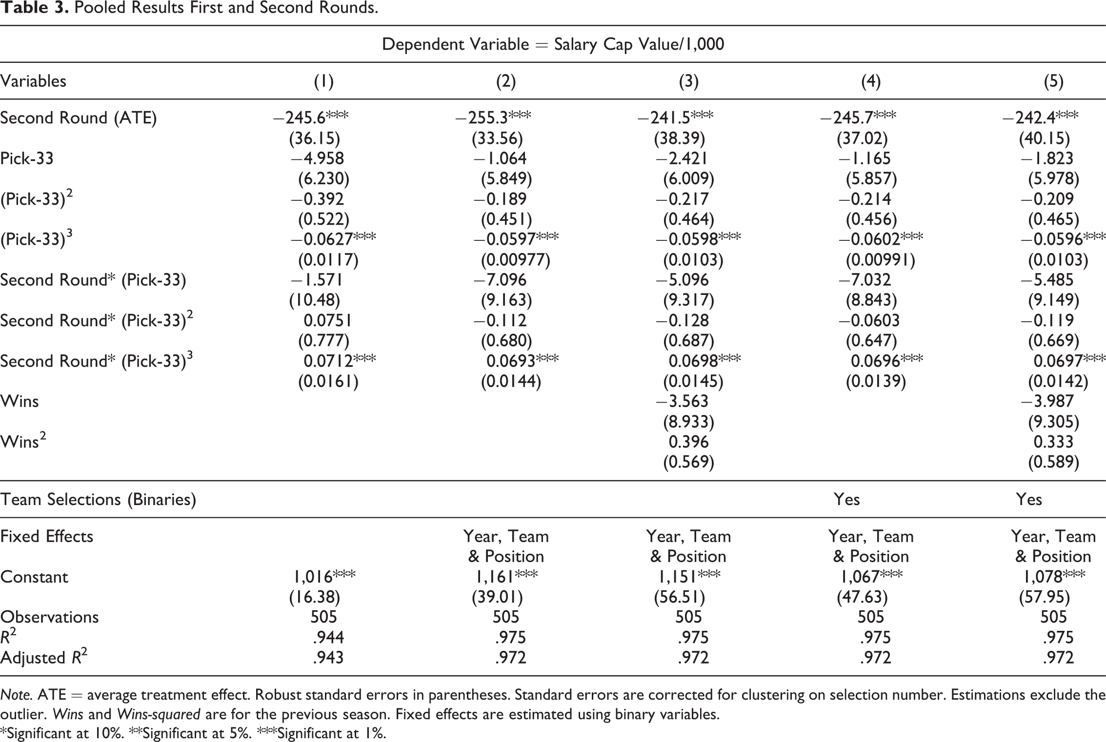
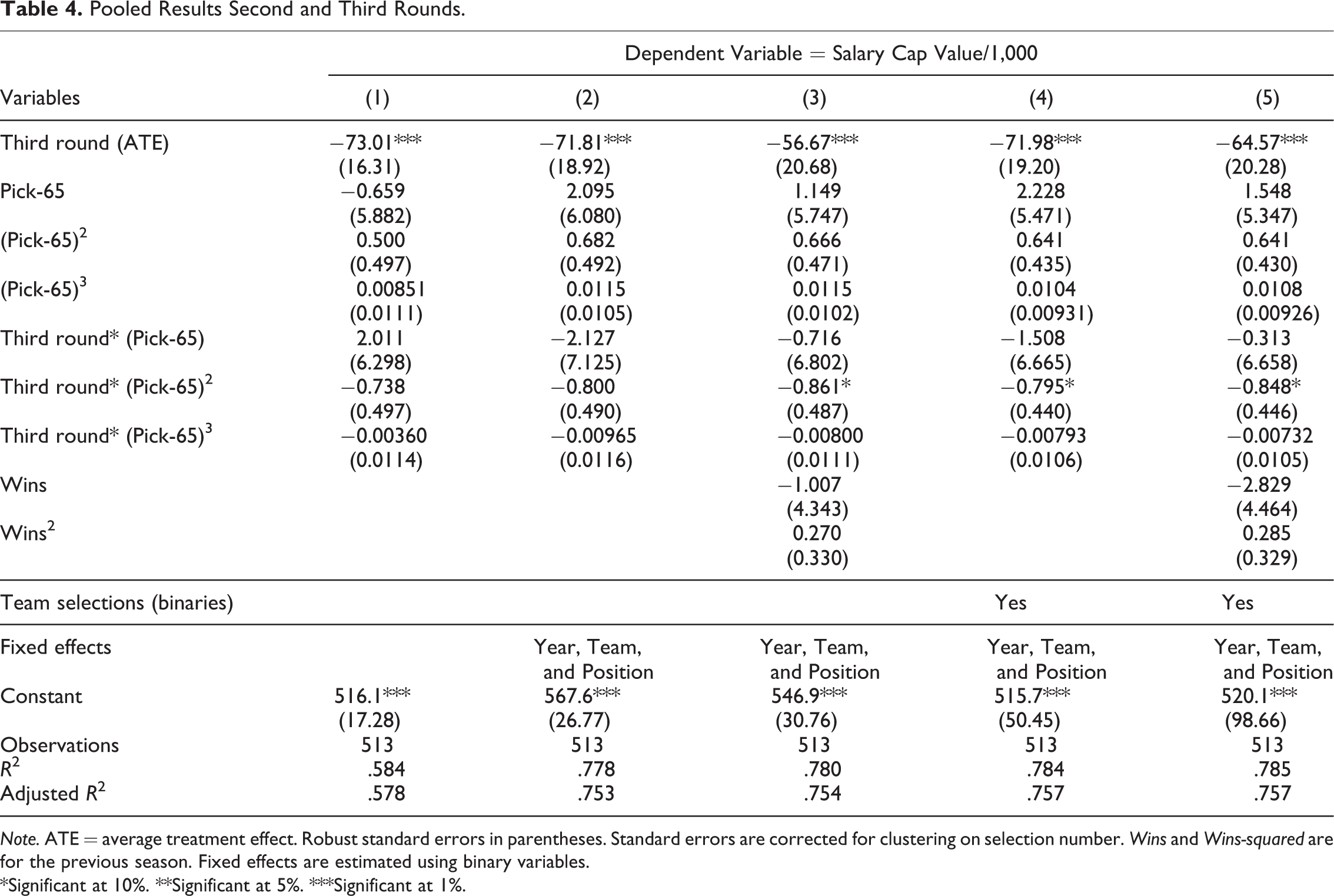
Pooled cubic regression results including year, team, and position fixed effects are reported in Table 3 for first and second round selections and Table 4 for second and third round selections. Since selection number is discrete, we follow Lee and Card (2008) and correct the standard errors for clustering on selection numbers. The ATE, or round effect, is statistically significant at 1% for all estimations. The first to second round baseline estimate is −US$255,300.⁹ This is even more surprising when considering the mean salary for the 33rd pick, the first selection of the second round, is US$702,680. Therefore, the first to second round effect is 36.3% of the average compensation of the first selection in the second round. The baseline second to third round ATE is −US$71,810. Since the mean salary cap value of pick number 65 is US$430,527, the estimated round effect is 16.7% of the average salary of the first pick in the third round.

Table 3.

Pooled Results First and Second Rounds.

Dependent Variable = Salary Cap Value/1,000
Variables	(1)	(2)	(3)	(4)	(5)
Second Round (ATE)	−245.6*** (36.15)	−255.3*** (33.56)	−241.5*** (38.39)	−245.7*** (37.02)	−242.4*** (40.15)
Pick-33	−4.958 (6.230)	−1.064 (5.849)	−2.421 (6.009)	−1.165 (5.857)	−1.823 (5.978)
(Pick-33)²	−0.392 (0.522)	−0.189 (0.451)	−0.217 (0.464)	−0.214 (0.456)	−0.209 (0.465)
(Pick-33)³	−0.0627*** (0.0117)	−0.0597*** (0.00977)	−0.0598*** (0.0103)	−0.0602*** (0.00991)	−0.0596*** (0.0103)
Second Round* (Pick-33)	−1.571 (10.48)	−7.096 (9.163)	−5.096 (9.317)	−7.032 (8.843)	−5.485 (9.149)
Second Round* (Pick-33)²	0.0751 (0.777)	−0.112 (0.680)	−0.128 (0.687)	−0.0603 (0.647)	−0.119 (0.669)
Second Round* (Pick-33)³	0.0712*** (0.0161)	0.0693*** (0.0144)	0.0698*** (0.0145)	0.0696*** (0.0139)	0.0697*** (0.0142)
Wins			−3.563 (8.933)		−3.987 (9.305)
Wins²			0.396 (0.569)		0.333 (0.589)
Team Selections (Binaries)				Yes	Yes
Fixed Effects		Year, Team	Year, Team	Year, Team	Year, Team
Fixed Effects		& Position	& Position	& Position	& Position
Constant	1,016*** (16.38)	1,161*** (39.01)	1,151*** (56.51)	1,067*** (47.63)	1,078*** (57.95)
Observations	505	505	505	505	505
R ²	.944	.975	.975	.975	.975
Adjusted R ²	.943	.972	.972	.972	.972

Note. ATE = average treatment effect. Robust standard errors in parentheses. Standard errors are corrected for clustering on selection number. Estimations exclude the outlier. Wins and Wins-squared are for the previous season. Fixed effects are estimated using binary variables.

*Significant at 10%. **Significant at 5%. ***Significant at 1%.

Table 4.

Pooled Results Second and Third Rounds.

	Dependent Variable = Salary Cap Value/1,000
Variables	(1)	(2)	(3)	(4)	(5)
Third round (ATE)	−73.01*** (16.31)	−71.81*** (18.92)	−56.67*** (20.68)	−71.98*** (19.20)	−64.57*** (20.28)
Pick-65	−0.659 (5.882)	2.095 (6.080)	1.149 (5.747)	2.228 (5.471)	1.548 (5.347)
(Pick-65)²	0.500 (0.497)	0.682 (0.492)	0.666 (0.471)	0.641 (0.435)	0.641 (0.430)
(Pick-65)³	0.00851 (0.0111)	0.0115 (0.0105)	0.0115 (0.0102)	0.0104 (0.00931)	0.0108 (0.00926)
Third round* (Pick-65)	2.011 (6.298)	−2.127 (7.125)	−0.716 (6.802)	−1.508 (6.665)	−0.313 (6.658)
Third round* (Pick-65)²	−0.738 (0.497)	−0.800 (0.490)	−0.861* (0.487)	−0.795* (0.440)	−0.848* (0.446)
Third round* (Pick-65)³	−0.00360 (0.0114)	−0.00965 (0.0116)	−0.00800 (0.0111)	−0.00793 (0.0106)	−0.00732 (0.0105)
Wins			−1.007		−2.829
Wins			(4.343)		(4.464)
Wins²			0.270		0.285
			(0.330)		(0.329)
Team selections (binaries)				Yes	Yes
Fixed effects		Year, Team, and Position	Year, Team, and Position	Year, Team, and Position	Year, Team, and Position
Constant	516.1*** (17.28)	567.6*** (26.77)	546.9*** (30.76)	515.7*** (50.45)	520.1*** (98.66)
Observations	513	513	513	513	513
R ²	.584	.778	.780	.784	.785
Adjusted R ²	.578	.753	.754	.757	.757

Note. ATE = average treatment effect. Robust standard errors in parentheses. Standard errors are corrected for clustering on selection number. Wins and Wins-squared are for the previous season. Fixed effects are estimated using binary variables.

*Significant at 10%. **Significant at 5%. ***Significant at 1%.

As previously mentioned, average team success and average within team selection number shift at the round cutoffs. Therefore, we include the number of previous season wins and the number of wins squared, to allow for a nonlinear effect of team success, and a vector of binary variables indicating a player’s within team selection number. The first to second round effect is −US$242,400 and the second to third round effect is −US$64,570.¹⁰ The results are robust to changes in team success and within-team selection number and support our RDD identification strategy.

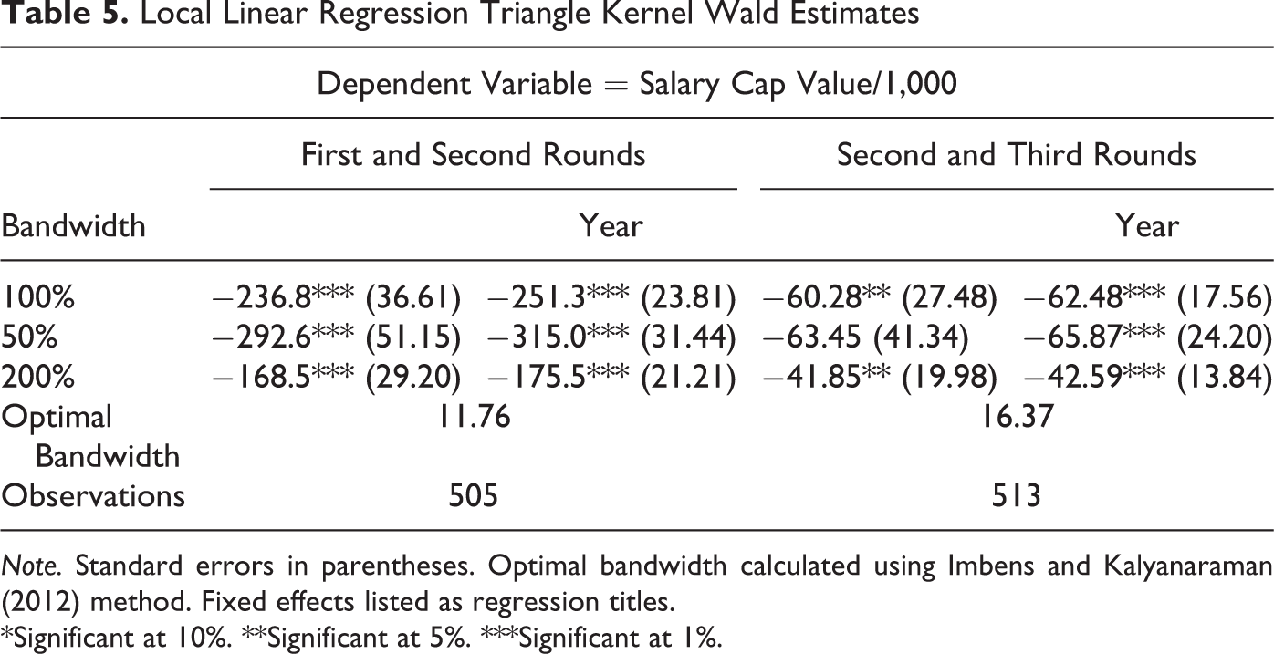
Local Linear Regression Results

We estimate the LATE using the triangular kernel and the Imbens and Kalyanaraman (2012) optimal bandwidth. We analyze the round effects both with and without year fixed effects. Local linear regression is normally estimated without additional covariates; however, year fixed effects are included for comparison, as there is clear impact of the year on salary cap value which is exogenous from the effect of selection number. The results are presented in Table 5. The first to second round discontinuity is robustly significant at 1%. It is robust to the selection of bandwidth and the inclusion of year fixed effects. Similar to the pooled regression results, the first to second round discontinuity is very large. The optimal bandwidth displays an LATE of −US$237,000 to −US$251,000.¹¹ The second to third round LATE using the optimal bandwidth is −US$60,000 to −US$62,000.

Table 5.

Local Linear Regression Triangle Kernel Wald Estimates

Dependent Variable = Salary Cap Value/1,000
	First and Second Rounds		Second and Third Rounds
Bandwidth		Year		Year
100%	−236.8*** (36.61)	−251.3*** (23.81)	−60.28** (27.48)	−62.48*** (17.56)
50%	−292.6*** (51.15)	−315.0*** (31.44)	−63.45 (41.34)	−65.87*** (24.20)
200%	−168.5*** (29.20)	−175.5*** (21.21)	−41.85** (19.98)	−42.59*** (13.84)
Optimal Bandwidth	11.76		16.37
Observations	505		513

Note. Standard errors in parentheses. Optimal bandwidth calculated using Imbens and Kalyanaraman (2012) method. Fixed effects listed as regression titles.

*Significant at 10%. **Significant at 5%. ***Significant at 1%.

Possible Mechanisms

Our study is similar to Lacetera, Pope, and Sydnor (2012), who find evidence of the left-digit bias in used vehicle prices, in that there is no actual treatment being administered at the cutoff points.¹² Therefore, we explore possible psychological mechanisms that may cause people to use rank-based groupings in decision making, thus creating the round effects. It is possible the round discontinuities are the result of the rookie salary cap. As previously mentioned, NFL teams are allotted a specific dollar amount to sign rookie players. Although the equation determining each team’s allotment is kept secret to the NFL, NFL general managers and players’ agents may have uncovered the mechanism to some degree. In fact, the CBA, which was supposed to run until 2012, explicitly states the rounds are considered in the rookie salary cap (National Football League, 2006). However, in the CBA discussion of rookie compensation, for purposes of incentive bonuses the first three rounds were grouped together. Therefore, it is possible the round discontinuities are an artifact of the secret equation, but unlikely.

A more plausible explanation is the theory of anchoring and adjustment, which has been shown in many situations (Ariely, Lowenstein, & Prelec, 2003; Northcraft & Neale, 1987; Tversky & Kahneman, 1974). Anchoring takes place when individuals focus on a particular, often irrelevant, piece of information. Given the anchor, additional information is used to make adjustments and decisions. If there is not substantial adjustment, the anchor will have a significant impact on decision making. For example, Ariely, Lowenstein, and Prelec (2003) asked individuals whether or not they would purchase several ordinary consumer products, one of which was a bottle of wine, for a price equal to the last two digits of their social security number. Individuals then stated their willingness to pay (WTP) for each good. The results show an individual’s social security number had a significant impact on their WTP. Teams and agents may be using the round as an anchor. Expected productivity is then adjusted based on selection number. Round discontinuities are created due to a lack of adjustment and the anchor being changed at the round cutoffs.

Another mechanism, which is very similar to anchoring and adjustment, is the use of focal points to facilitate coordination (Schelling, 1957, 1960). Schelling discusses focal points in situations where agents cannot communicate, but are required to coordinate. The classic example is being told you must meet a person in New York City and the two of you must arrive at the same location at the same time. Here, people often coordinate using focal points, which are common meeting places at common times. Rookie compensation is a coordination situation, as teams bargain with players’ agents. Teams and agents may use the round as a focal point or common starting point for negotiations. At the round cutoffs, the focal point shifts, which may result in the observed discontinuities. It is important to note that any possible alternate explanation must generate discontinuities uniquely at the round cutoffs.

Conclusion

The NFL draft is analyzed to examine the effect of rank-based groupings on decision making. The rounds of the draft are simply groupings of players based on selection number. As rank-based groupings are uninformative signals given the rank is observed, the rounds should be ignored in decision making. Discontinuities in rookie compensation at the round cutoffs are evidence of a causal effect of the draft rounds on compensation. Thus, they are evidence of the use of rank-based groupings in high-stakes decision making.

A sharp RDD analysis of the round cutoffs reveals very large and robustly significant round effects on rookie salary cap value. The analysis uses both pooled cubic and local linear regressions. The estimated first to second round effect is −US$240,000 to −US$250,000. The estimated second to third round effect is −US$60,000 to −US$70,000. Both effects are robust to team success and within-team selection number, which vary between rounds. Later round effects could not be estimated using RDD because there are no consistent cutoffs between rounds throughout years.

Evidence of the effect of rank-based groupings on decision making in the NFL is important for several reasons. First, rookie compensation comprises a large portion of career earnings for players. Heuristic thinking in the compensation of rookies has a major impact on lifetime earnings, especially for those near the round cutoffs. Second, the use of a sharp RDD quasi-experimentally estimates the causal relationship. Third, the results are derived from real-world decision making. Finally, the use of rank-based groupings is shown in a market with very high stakes.

Footnotes

Appendix

Table A1.

Number of Teams With Multiple Selections in a Given Round.

	Round
Year	1	2	3
2002	1	7	4
2003	4	3	4 (1)
2004	5	8 (1)	3
2005	4	3	7
2006	3	3 (1)	6 (1)
2007	2	6 (1)	7 (1)
2008	5	4 (2)	9 (4)
2009	4	7 (2) [1]	5

Note. The number of teams with two selections in a given round. Numbers in parentheses indicate the number of teams with three selections in the given round. Numbers in square brackets indicate the number of teams with four selections in the given round.

Author’s Note

I am grateful for the feedback of Joshua Tasoff, Thomas Kniesner, and Serkan Ozbeklik. All errors are mine alone.

Declaration of Conflicting Interests

The author(s) declared no potential conflicts of interest with respect to the research, authorship, and/or publication of this article.

Funding

The author(s) received no financial support for the research, authorship, and/or publication of this article.

Notes

References

Ariely

Lowenstein

Prelec

(2003). Coherent arbitrariness: Stable demand curves without stable preferences. Quarterly Journal of Economics, 118, 73–106.

Berri

D. J.

Simmons

(2011). Catching a draft: On the process of selecting quarterbacks in the national football league amateur draft. Journal of Productivity Analysis, 35, 37–49.

Cheng

M.-Y.

Fan

Marron

J. S.

(1997). On automatic boundary corrections. Annals of Statistics, 25, 1691–1708.

Fan

Gijbels

(1996). Local polynomial modelling and its applications. New York, NY: Chapman and Hall.

Florio

(2011, 7 31). Sources: Disclosure of rookie scale formula by NFLPA nearly blew up settlement. NBC Sports. Retrieved from http://profootballtalk.nbcsports.com/2011/07/31/sources-disclosure-of-rookie-scale-formula-by-nflpa-nearly-blew-up-settlement/

Hendricks

DeBrock

Koenker

(2003). Uncertainty, hiring and subsequent performance: The NFL draft. Journal of Labor Economics, 21, 857–886.

Imbens

G. W.

Kalyanaraman

(2012). Optimal bandwidth choice for the regression discontinuity estimator. Review of Economic Studies, 79, 933–959.

Imbens

G. W.

Lemieux

(2008). Regression discontinuity designs: A guide to practice. Journal of Econometrics, 142, 615–635.

Kahn

L. M.

(1992). The effects of race on professional footballers’ compensation. Industrial and Labor Relations Review, 45, 295–310.

10.

Karimian

(2011, 3 25). NFL announces compensatory picks for april’s draft. USA Today. Retrieved from http://content.usatoday.com/communities/thehuddle/post/2011/03/nfl-draft-compensatory-picks-announced/1

11.

Keefer

Q. A. W.

(2013). Compensation discrimination for defensive players: Applying quantile regression to the national football league market for linebackers. Journal of Sports Economics, 14, 23–44.

12.

Lacetera

Pope

D. G.

Sydnor

J. R.

(2012). Heuristic thinking and limited attention in the car market. American Economic Review, 102, 2206–2236.

13.

Lee

D. S.

(2008). Randomized experiments from non-random selection in U.S. house elections. Journal of Econometrics, 142, 675–697.

14.

Lee

D. S.

Card

(2008). Regression discontinuity inference with specification error. Journal of Econometrics, 142, 655–674.

15.

Lee

D. S.

Lemieux

(2010). Regression discontinuity designs in economics. Journal of Economic Literature, 48, 281–355.

16.

Ludwig

Miller

D. L.

(2007). Does head start improve children’s life chances? Evidence from a regression discontinuity design. Quarterly Journal of Economics, 122, 159–208.

17.

Massey

Thaler

R. H.

(2010). The loser’s curse: Overconfidence vs. market efficiency in the national football league draft. Mimeo: University of Chicago.

18.

Mirabile

M. P.

(2007). The NFL rookie cap: An empirical analysis of one of the NFL’s most closely guarded secrets. The Sport Journal, 10. Retrieved from http://www.thesportjournal.org

19.

National Football League. (2006). NFL CBA 2006-2012. Retrieved from http://static.nfl.com/static/content/public/image/cba/nfl-cba-2006-2012.pdf

20.

National Football League. (2008). NFL Owners opt out of CBA. Retrieved from http://www.nfl.com/news/story?id=09000d5d80868b78&template=without-video&confirm=true

21.

Nichols

(2007). Causal inference with observational data. The Stata Journal, 7, 507–541.

22.

Northcraft

G. B.

Neale

M. A.

(1987). Experts, amateurs, and real estate: An anchoring-and-adjustment perspective on property pricing decisions. Organizational Behavior and Human Decision Processes, 39, 84–97.

23.

Pro Football Reference. (2011). NFL draft history and AFL drafts. Retrieved http://www.pro-football-reference.com/draft/

24.

Salganik

M. J.

Peter

Watts

D. J.

(2006). Experimental study of inequality and unpredictability in an artificial cultural market. Science, 311, 854–856.

25.

Schelling

(1960). The strategy of conflict. Cambridge, MA: Harvard University Press.

26.

Schelling

(1957). Bargaining, communication, and limited war. Conflict Resolution, 1, 19–36.

27.

Simmons

Berri

D. J.

(2009). Does it always pay to specialize? The story from the gridiron. Review of Industrial Organization, 34, 81–98.

28.

Tversky

Kahneman

(1974). Judgment under uncertainty: Heuristics and biases. Science, 185, 1124–1131.

29.

USA Today. (2011). USA today salaries databases: National football league salaries. Retrieved from http://content.usatoday.com/sportsdata/football/nfl/salaries/team?loc=interstitialskip

30.

van der Klaauw

(2002). Estimating the effect of financial aid offers on COLLEGE enrollment: A regression-discontinuity approach. International Economic Review, 43, 1249–1287.

31.

Weber

Camerer

C. F.

(1998). The disposition effect in securities trading: An experimental analysis. Journal of Economic Behavior & Organization, 33, 167–184.