Does the Threat of Suspension Curb Dangerous Behavior in Soccer? A Case Study From the Premier League

Abstract

Using data from the 2011-2012 season of the Premier League, we study empirically and theoretically the impact of soccer suspension rules on the behavior of players and referees. For players facing a potential one-game suspension, being one versus two yellow cards away from the suspension limit results in an approximate 12% reduction in fouling, while for those facing a potential two-game suspension, the reduction is approximately 23%. The probability such players receive a yellow card is also reduced. In addition, we find some evidence of slight referee bias for the home team in the dispensing of penalty cards, but not in the calling of fouls. Finally, we develop a theoretical framework for investigating the effects of suspension rules on the number of fouls committed. Within this framework, we investigate how policy instruments such as referees’ propensity to give out yellow cards or their consistency in giving them out affect the impact of suspension rules.

Keywords

logistic regression quasi-Poisson regression yellow cards deterrence soccer decision-making

Introduction

In this article, we quantitatively evaluate the effect of suspension rules on players’ behavior in soccer. Soccer, like many other forms of football, features situations when two players collide in an attempt to control a ball. Such collisions are potentially dangerous to players. In extreme cases, they can result in injuries so serious that they threaten the players’ future careers. In order to mitigate such outcomes and maintain the integrity of the game, various tournament and league organizers introduce punishment schemes to deter players from dangerous play. In soccer, a dangerous play is typically punished by showing the player a yellow card, which goes on the player’s record (he is “booked”). Accumulation of a certain number of yellow cards in a season results in the player being suspended for one or more games. Our goal in this article is to evaluate the impact of the threat of such suspensions on players’ behavior.

Specifically, we analyze a unique, player-game-level data set from the English Premier League to address the following three questions: (1) Under the current suspension rules, what affects the number of fouls committed? (2) Under the current suspension rules, what affects the probability of getting a penalty card? and (3) How would the number of fouls committed differ if the suspension rules changed?

First, we estimate the effect that the threat of missing a game has on a player’s propensity to commit a foul. In order to do so, we use a Poisson regression where we estimate the expected number of fouls committed in a game, as a function of the number of yellow cards the player can still receive before being suspended, as well as the player’s unobservable characteristics (fixed effects), and a large number of control variables. Our results suggest that if a player is only one yellow card away from suspension instead of two, the expected number of fouls he would commit in the game drops by 12% if he faces a one-game suspension and 23% if he faces a two-game suspension.

Second, we use a logistic regression to estimate the probability p of a player receiving a penalty card. Our results show that if a player is only one yellow card away from suspension instead of two, his odds (p divided by 1 − p) of getting a penalty card are reduced by 50% if he faces a one-game suspension and by 70% if he faces a two-game suspension.

Finally, we develop a dynamic model of a player’s optimal behavior and show that our empirical results are in line with the predictions of the economic theory. We calibrate model parameters (as much as possible) and use the model to analyze the effect of suspension rules on player behavior—not only in the games just before possible suspension, but even early in the season. This framework allows us to investigate the impact of changing the suspension rules, something impossible to do using the data alone (Lucas, 1976).

We want to point out that it is not obvious a priori what the effects of the suspension rules on player behavior might be. The direct effect is that the threat of suspension makes the player more cautious. There can be, however, another strategic effect. In 2010, two Real Madrid players strategically received yellow cards for delaying a game, only to miss the upcoming, last game of a group stage, and have their records clean for the more important knockout stage that their team had secured earlier. Another aspect to consider is that whether to book a player is ultimately the referee’s decision on the field. It is quite plausible that a referee, knowing a player is facing a possible one-game suspension, may alter his decision about booking in a nonobvious situation (when a foul is borderline dangerous).

The outline of the article is as follows: The second section discusses the relevant literature, while the third section contains relevant background information about the game of soccer and the English Premier League. The fourth section describes the data set utilized in this study. The Poisson and logistic regression models are explained and discussed in the fifth section, while the dynamic modeling framework is set forth in the sixth section. The last section gives some concluding remarks and avenues for future research.

Relation to the Literature

Several authors have studied the impact of a red card on outcome of the match (e.g., Bar-Eli, Tenenbaum, & Geister, 2006; Ridder, Cramer, & Hopstaken, 1994; Vecer, Kopriva, & Ichiba, 2009). Dobson, Goddard, and Staehler (2014) used a Tullock contest model to predict levels of effort in the English Premier League, with data on fouls and yellow and red cards used to reflect the effort of teams. Team-level data were used for matches played between the 2001-2002 and 2006-2007 seasons. Snyder (2013) uses individual-level Premier League data from the 2011-2012 season to predict game outcomes in the context of sports betting. We use this same data to answer a different question: How much, if at all, does the Premier League’s suspension rule curb fouling? A similar question was asked by del Corral, Prieto-Rodriguez, and Simmons (2010), who studied whether Spain’s 1995 rule change awarding 3 points for a win instead of 2 affected the team-wide probability of a red card. Garicano and Palacios-Huerta (2005) studied the same question as del Corral et al. (2010) but used data from a different year. Stride, Patterson, and Thomas (2011) gathered data on fouls in the 2010 World Cup tournament, both those caught by referees and those that should have been. They modeled foul counts with the Poisson distribution and utilized a dispersion parameter to account for non-Poisson variance. They found that position, international experience, and the stage of tournament were important predictors of fouls. The World Cup, however, has different suspension rules than the Premier League, and it does not seem that the effect of these rules on fouls was considered (Stride et al., 2011, is unpublished at the time of this writing).

Our article is closely related to the economic literature on crime¹ and deterrence. McCormick and Tollison (1984) evaluate the effect of adding the third referee in basketball on the number of fouls in the National Basketball Association. They find the additional referee matters: the number of fouls by players dropped. A similar point is made by Tella and Schargrodsky (2004) who show that an increase in the number of police reduces the number of nonviolent crimes committed. Both studies suggest that unwanted behavior declines if the probability of being punished increases. Our result confirms that observation: The more yellow cards the player has accumulated (i.e., the more likely the player is to be suspended), the fewer fouls he commits. Finally, Kessler and Levitt (1999) address whether jail sentences reduce crime through deterrence, that is, by affecting potential criminals’ behavior. Their findings suggest that the threat of punishment mitigates unwanted behavior. In our article, we confirm that effect and quantify it in the context of punishment cards and suspension rules in soccer.

A special subset of the crime literature concerns the effects of “three-strikes” legislation enacted in California and elsewhere. Such laws impose harsh punishments on frequent offenders. Early analyses of the legislation’s effects (Greenwood et al., 1994; Zimring, Kamin, & Hawkins, 1999) considered only partial deterrence, the deterrence of offenders who had already received two strikes. A more sophisticated analysis by Shepherd (2002) shows that this underestimates the true effect of the laws, since three-strikes laws also deter individuals contemplating their first offense. We likewise expect that the effects of suspension rules in the Premier League will extend beyond players who are just one card away from an accumulation limit. Helland and Tabarrok (2007), taking advantage of the randomization of trial outcomes, found that California’s three-strikes laws reduce felony arrest rates of criminals with two strikes by approximately 17–20%. Similarly, as part of our analysis, we estimate the effect, given the suspension rules, of being one versus two yellow cards away from the accumulation limit. In his comprehensive review of the evidence regarding deterrence, Nagin (2013) suggests that certainty of punishment may have a greater impact on behavior than severity of punishment. In the structural model of the “Theoretical Model” section, in addition to incorporating the severity of punishment, we include a parameter that captures the certainty of punishment.

Of course, whether a player gets called for a foul or receives a penalty card depends not only on his behavior but also on the referee’s. Morgulev, Azar, Lidor, Sabag, and Bar-Eli (2014) show that basketball players fall intentionally in order to deceive referees that they are being fouled. Such deception in soccer weakens the link between a player’s actual aggressiveness and the probability he would receive a yellow card. A play that is not dangerous may be called as one, and a truly aggressive play may be misinterpreted as “diving”—an intentional fall by the other player. We take these problems into consideration in our structural model of optimal yellow card accumulation.

Another important factor in referees’ behavior is the possibility of favoring a home team. Indeed, Dawson, Dobson, Goddard, and Wilson (2007) found that the tendency for home teams to incur fewer penalty cards than away teams was best explained by referee bias. Home-field bias was also found by Sutter and Kocher (2004) in a study of the German Bundesliga. In addition, Sutter and Kocher (2004) confirmed the finding by Garicano, Palcios-Huerta, and Predergast (2005) that extra time was awarded in a way that favored the home team. The evidence for referee bias is not limited to what has been discovered by statistical analysis of match data, however compelling this evidence is; it has also been confirmed by experimentation. Using video clips from English Premier League games, Nevill, Balmer, and Williams (2002) conducted an experiment in which 40 referees were asked to classify tackles as regular or irregular. Half of the referees were shown the clips with the audience muted while the other half were able to hear the audience. Referees who could hear the audience were more reluctant to classify home team tackles as irregular and their decisions correlated better with the “game-time” decisions than did those by referees who watched the muted clips. Taken together, these studies constitute rather strong evidence that referees tend to favor the home team when dispensing penalty cards. We therefore take venue into account in all empirical models presented herein.

Background Information

Since we study the impact of certain types of punishment rules on player behavior, we will now briefly outline the different types of offenses and individual punishments in soccer. We will also describe in detail the Premier League suspension rules.

Yellow Cards Rules and Offenses Punishable

The individual punishment we focus on is a yellow card. A yellow card is used by a referee to officially caution a player who commits a certain offense. It goes on the player’s official record (the player is booked). Two yellow cards in a game turn into a red card, which expels the player for the rest of the game, and his team plays with one man down. The player must also sit out the next game. International Federation of Association Football (FIFA) specifies the offenses that are punishable with a yellow card. These are (1) unsporting behavior; (2) dissent by word or action; (3) persistent infringement of the Laws of the Game; (4) delaying the restart of play; (5) failure to respect the required distance when play is restarted with a corner kick, throw-in, or free kick; (6) entering or reentering the field of play without the referee’s permission; and (7) deliberately leaving the field of play without the referee’s permission. The unsporting behavior includes dangerous fouls, removing a jersey after a goal celebration, or simulating actions in order to deceive a referee (e.g., diving in the penalty box in order to be given a penalty kick).

By far, the most common offense punishable by a yellow card is dangerous play. The use of yellow cards to punish dangerous play has evolved over the last 30 years to make the game safer for players involved. It includes codification of fouls that automatically result in a yellow card (e.g., an incidental tackle from behind). In addition to that, different organizations introduce additional game suspensions for players who have a record of dangerous play in multiple games. For instance, in the FIFA World Cup and in the Union of European Football Associations Champions League, two yellow cards received in two different games of the same stage result in a suspension of a player for one match.

Suspension Rules in the Premier League for 2011-2012 Season

Like any other organization, the Premier League has its own suspension rules. The season starts in August and lasts till May, with each of 20 teams playing every other team twice (once at home, once away) for a total of 38 games. If a player accumulates five yellow cards before December 31, he is suspended for one game. If he accumulates 10 yellow cards before the second Sunday in April, he is suspended for two games. Finally, if he accumulates 15 yellow cards before the end of the season, he is suspended for three games (or the rest of the season if there are fewer than three games remaining). All suspensions take place immediately following the game.

We had to pay special attention to red cards. In our data (see “Data” section), if a player receives two yellow cards in a game, it is coded as one red card and zero yellow cards. If a player receives a straight red card, it is coded as one red card as well and the player may or may not have a yellow card as well. In the Premier League, if a red card is a result of two yellows, then the player leaves the field, misses the very next game (because of the red card), but he is still booked for two yellow cards which go on his record toward the possible future suspension.

Incentives Caused by Suspension Rules

These suspension rules create a complex set of incentives for a player. First of all, as the three-strikes literature suggests, the very possibility of future suspension should curb card-worthy behavior for all players, regardless of how close they are to the cutoff (Shepherd, 2002). We expect, however, that as a player nears the accumulation limit, he will be increasingly likely not to foul. Being one or two yellows away from the limit may constitute special situations since the player is now “one strike” away in the sense that one bad act could bring him to the limit.

All else being equal, we expect the incentives against fouling to be stronger when facing a longer suspension. In practice, however, all else isn’t equal: When accumulating yellows toward a shorter suspension, players are also accumulating yellows toward the longer one as well. Thus, the measured effect of facing a one-game suspension includes the effect of a looming possible two-game suspension. In addition, there should be some temporal effect, since a player with three yellows to give and one game before the deadline will tend to be more aggressive than he would be if he had eight games to go. In the “Regression Models” section, we introduce regression models which we feel do an adequate job of teasing out the effects of these incentives, while the structural theoretical model presented in the “Theoretical Model” section, by explicitly incorporating the dynamic aspect of the incentives, allows one to explore what would happen if the suspension rules were changed.

Data

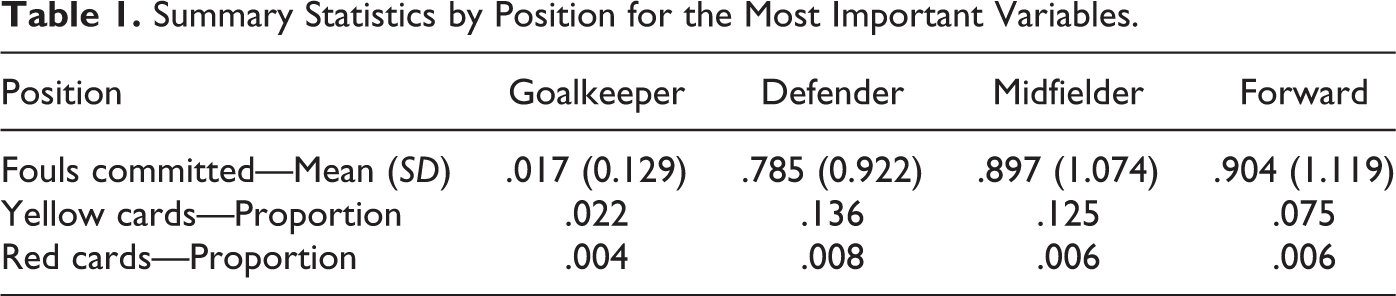
To estimate the effect of the Premier League’s cumulative penalty card suspension rules, we utilize a very rich data set containing individual player data from each game of the 2011-2012 season. The data set was released in the summer of 2012 by Manchester City Football Club in collaboration with the data gathering company Opta in order to encourage soccer analytics. For each player in each game, frequency counts for some 200 different events, ranging from successful passes to duels won to goals scored, are recorded. (A more detailed description of the individual variables we included in our analysis is available in Appendix. For a detailed description of the variables not included, see Opta, 2012.) These data are analyzed on various Internet blogs (e.g., Bime, 2012; Brown, 2012; Ramineni, 2012), but no analysis has focused on estimating the effect of the suspension rules on player or referee behavior. Snyder (2013) used the data to predict game outcomes (home loss, tie, or home win) in the context of sports betting. Table 1 gives summary statistics by position for the most important variables. Since each row of the data set corresponds to a player–game combination, these can be thought of as the league-wide per game averages. The data set included one row for every unique player–game combination for a total of 10,369 rows. There were 539 unique players from 20 teams, each player playing anywhere from 1 to 38 games. Every team played every other team twice, once at home and once away.

Table 1.

Summary Statistics by Position for the Most Important Variables.

Position	Goalkeeper	Defender	Midfielder	Forward
Fouls committed—Mean (SD)	.017 (0.129)	.785 (0.922)	.897 (1.074)	.904 (1.119)
Yellow cards—Proportion	.022	.136	.125	.075
Red cards—Proportion	.004	.008	.006	.006

Regression Models

We model the effect of the suspension policy on two outcomes of interest: the number of fouls committed and the probability of receiving a penalty card (yellow or red). We suspect that players close to the card limit will behave less aggressively and therefore commit fewer fouls and incur fewer penalties. Because number of fouls committed takes on integer values, we use Poisson regression instead of the more common linear regression. (Technically, we use quasi-Poisson regression, which allows for more flexibility in the variation of observations about their mean than does regular Poisson regression.) For modeling the probability of receiving a penalty card, we use logistic regression.

As a result of their position and/or style of play, some players are inherently more aggressive than others. We account for this by including a different intercept for each player in both models. We assume that this latent level of aggressiveness remains constant across games, but believe that there may also be game-specific increases or decreases in aggression for various reasons. For example, a player who typically is not aggressive may be agitated by someone else committing fouls against him, leading to more fouls committed than normal. Or perhaps a player gets the ball stolen, which could increase the probability that he will foul in retaliation. We account for these circumstantial, game-specific changes in aggression by including appropriate covariates in both models.

Model for Number of Fouls (Quasi-Poisson Regression)

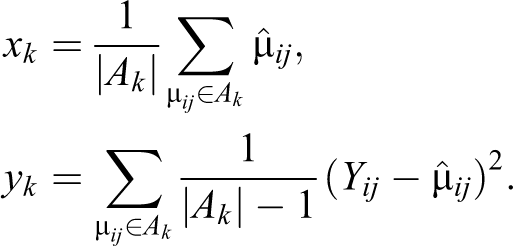
In Poisson regression, the expected number of fouls committed by player i in game j is

μ_{i j} = \exp {α_{i} + x_{i j}^{T} β},

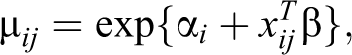
where α_i is the fixed effect (inherent level of aggression) for player i, x_ij are the covariates for player i in game j, and β is a vector of regression coefficients common to all players. The number of fouls Y_ij committed by player i in game j is assumed to follow a Pois(μ _ij ) distribution. This type of model is sometimes called a Poisson log-linear model because log(μ _ij ) is linear in the model parameters β (Agresti, 2002, pp. 125–126). Poisson regression is more appropriate than, say, ordinary least squares for modeling foul counts because the Poisson distribution has the nonnegative integers as its support, whereas the normal distribution covers the whole real line.

A special property of the Poisson distribution is that its mean and variance are equal. In practice, however, count data do not always exhibit this property. One solution that retains many of the advantages of Poisson regression is to introduce a dispersion parameter φ and require E(Y_ij) = μ_ij and $Var (Y_{i j}) = ϕ μ_{i j}$ (Agresti, 2002, pp. 149–151). This can be seen as a relaxation of the usual assumption that $Y_{i j} \sim Pois (μ_{i j})$ , and the technique is known as quasi-Poisson regression. In their analyses of classic and tactical foul counts, Stride et al. (2011) also used quasi-Poisson regression. In the “Results” section, we use a graphical method to demonstrate that the quasi-Poisson model fits our data quite well.

We now turn our attention to the selection of covariates to be included in our model. We created three new variables and combined these in various ways in order to tease out effects of the Premier League’s cumulative yellow suspension rules. The new variables are Yellows.To.Give, Suspension.Duration, and Weeks.Until.Cutoff.

Yellows.To.Give refers to the number of yellow cards a player may incur (at the start of the game in question) before a suspension is warranted. Thus, if the date is on or before December 31, 2011, and a player has received four yellow cards, then Yellows.To.Give = 1, because once he receives one more yellow card, he has earned a suspension. If the date is on or before April 8, 2012, and the player has received seven yellow cards, then Yellows.To.Give = 3. When Yellows.To.Give is low, we believe a player will be more careful not to foul. If, in the course of a match, a player receives a number of yellow cards exceeding Yellows.To.Give, then he will be suspended for a number of games equal to Suspension.Duration, and Yellows.To.Give will be reset to the appropriate quantity at the start of the next game in which he participates. We expect that as the severity of the potential suspension increases, the propensity to foul should decrease.

We believe that Yellows.To.Give equaling 1 or 2 could constitute special situations (since one bad play results in suspension), the effects of which we would like to estimate separately for each suspension severity level. We constructed four additional variables to capture the effects of these special situations:² Y1S1, Y1S2, Y2S1, and Y2S2, where YiSj takes the value 1 if Yellows.To.Give equals i and Suspension.Duration equals j and the value 0 otherwise. When Yellows.To.Give exceeds 2, we require Yellows.To.Give and Suspension.Duration to affect the (log of) expected number of fouls linearly and independently by including Yellows.To.Give.Linear = Yellows.To.Give × I(Yellows.To.Give > 2) and Suspension.Duration.Linear = Suspension.Duration × I(Yellows.To.Give > 2) in the model.

Weeks.Until.Cutoff measures the number of weeks until the cutoff date for the next potential suspension. For example, suppose a player incurs his fifth cumulative yellow card on November 13, 2011, and is subsequently suspended for one game on November 20. For this player, Weeks.Until.Cutoff on November 13 is the number of weeks until December 31, but Weeks.Until.Cutoff on November 27 is the number of weeks until April 8. We expect players with more games to play before the suspension cutoff will tend to foul less, resulting in a negative coefficient.

There are, of course, other ways to incorporate these constructed variables into a model. For instance, one could assume that the (log of) expected number of fouls grows linearly in Yellows.To.Give, giving no special treatment to cases where a player is one card away from suspension. Or, instead of including a linear effect for Weeks.Until.Cutoff as we have done, one could use Yellows.To.Give/Weeks.Until.Cutoff to try to account for the fact that being three yellows away from a suspension means something different to someone one game away from the cutoff than to someone, say, eight games away. Having fit a number of similar models to this data set, we can say that the main conclusions we draw are robust to these choices. In short, we recognize that all models are approximations of reality and contend that ours is no less reasonable an approximation than any other.

Decisions to include specific control covariates were based on amateur knowledge of the game of soccer and the practical and statistical significance of the corresponding coefficients. We note that the estimates for the coefficients of interest were robust with regard to choices at the margins, due, we suspect, to the lack of multicollinearity among the covariates. Although previous literature suggested inclusion of player position, this was deemed unnecessary in light of the fact that an intercept was included for each player. The same holds true for amount of international experience as measured by number of “caps,” that is, appearances in an international game, which was found by Stride et al. (2011) to be a good predictor of number of fouls committed in the 2010 World Cup. Stride et al. suggest that fouls increase as stage increases, which they took as a proxy for the importance of the match increasing, but the Premier League season is a double round–robin tournament, not an elimination tournament, so it is not clear what the analogous variable to include would be. We tried including days since start of season with the thought that later games might be more important, but this turned out to be neither practically nor statistically significant, so it was excluded. We also tried but excluded the difference in the two teams’ end-of-season rankings for the same reason. (Weekly updated mid-season rankings would arguably have been more appropriate, but these were unavailable and would correlate quite strongly with end-of-season rankings anyhow.) Venue (Home/Away) was retained in the model despite its negligible effect because it was of secondary interest to determine whether this impacted the number of fouls called. Match.Differential, which is the score of the player’s team minus the score of the opposing team, was likewise retained in the model despite its negligible effect.

Model for Probability of Penalty Card (Logistic Regression)

We used the same set of covariates to model the probability of receiving a penalty card (yellow or red), except that the number of total fouls committed was also included as a predictor. We would like to discern whether referees treat players differently who are close to being suspended, but from these data alone we regrettably cannot disentangle changes in a player’s propensity to commit card-worthy offenses from changes in the referee’s propensity to book the player. However, under the assumption that players are no less aggressive at home than away (or that any such differences are captured by the control variables), a significant negative coefficient for Venue would confirm the home-field bias in refereeing that has been noted in the literature (see “Relation to the Literature” section herein).

Results

The results for Model 1 (fouls committed) can be seen in Table 2. Standard errors were computed using a dispersion parameter equal to .724 (see below for some discussion of this quantity). The most important finding is that when Yellows.To.Give decreases, propensity to foul decreases. For instance, when a player is one yellow card away from a one-game suspension, his expected number of fouls is $\exp (- .3446 + .2199) = 88 %$ of what it would be if he were two yellows away. Similarly if a player were one yellow card away from a two-game suspension, the expected number of fouls is just 77% of what it would be were he two yellows away from the limit. We also see that, regardless of the number of yellows a player is away from suspension, as the severity of suspension increases, the expected number of fouls decreases, as expected. Table 3 summarizes these effects by giving the expected number of fouls normalized by the expected number of fouls if Yellows.To.Give = 3 and Suspension.Duration = 1. The 88% and 77% can be recovered by taking .76/.86 and .57/.74, respectively. The last of our constructed variables, Weeks.Until.Cutoff, has a negative effect on propensity to foul, as expected: With each passing week, the number of expected fouls increases about 1%.

Table 2.

Results for the Quasi-Poisson Regression Model (Dependent Variable: Number of Fouls Committed).

Variable name	Estimate	SE	$\Pr (> \| t \|)$
Weeks.Until.Cutoff	−.0093	.0023	.0000
Y1S1	−.3446	.0876	.0001
Y2S1	−.2199	.0601	.0003
Y1S2	−.6225	.2131	.0035
Y2S2	−.3682	.2111	.0811
Yellows.To.Give.Linear	.0662	.0105	.0000
Suspension.Duration.Linear	−.2645	.0423	.0000
Match.Differential	−.0039	.0056	.4872
Total.Successful.Passes.All	.0033	.0008	.0001
Total.Fouls.Won	.0302	.0114	.0080
Interceptions	.0251	.0072	.0005
VenueHome	−.0092	.0196	.6398
Blocked.Shots	.0428	.0167	.0106
Unsuccessful.Dribbles	−.2218	.0118	.0000
Tackles.Won	.0250	.0102	.0140
Total.Clearances	.0124	.0047	.0083
Challenge.Lost	−.1745	.0120	.0000
Duels.lost	.2357	.0042	.0000
Duels.won	−.0139	.0061	.0222

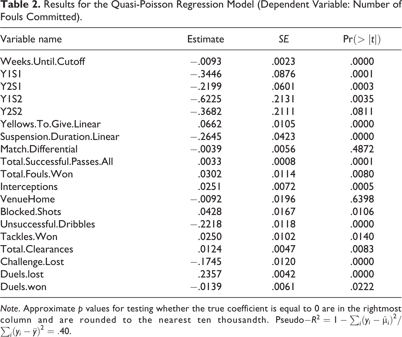
Note. Approximate p values for testing whether the true coefficient is equal to 0 are in the rightmost column and are rounded to the nearest ten thousandth. $Pseudo- R^{2} = 1 - \sum_{i} {(y_{i} - {\hat{μ}}_{i})}^{2} / \sum_{i} {(y_{i} - \bar{y})}^{2} = .40$ .

Table 3.

Expected Number of Fouls Divided by Expectation When Yellows.To.Give = 3 and Suspension.Duration = 1.

	Suspension.Duration
Yellows.To.Give	1	2	3
1	0.76	0.57	NA
2	0.86	0.74	NA
3	1.00	0.77	0.59
4	1.07	0.82	0.63
5	1.14	0.88	0.67

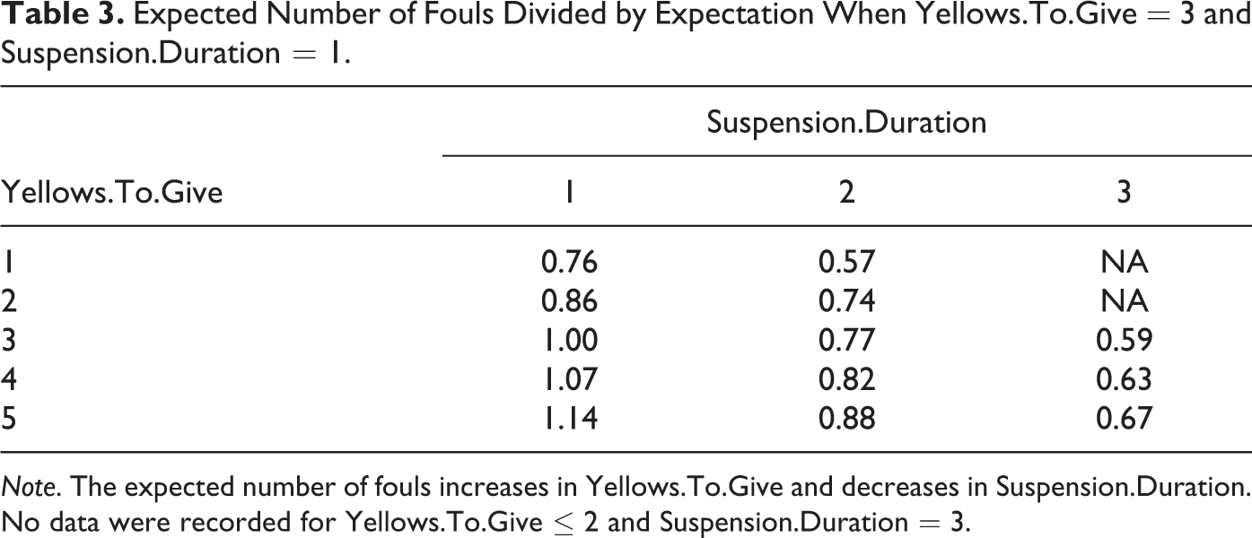
Note. The expected number of fouls increases in Yellows.To.Give and decreases in Suspension.Duration. No data were recorded for Yellows.To.Give ≤ 2 and Suspension.Duration = 3.

Several of the control variables’ effects are large enough to warrant mention. Losing an additional duel increases the number of expected fouls by 27% (for reference, strikers have the highest mean of 4.7 duels lost per game). Losing an additional challenge decreases expected fouls by 16% (midfielders average .65). Having an additional unsuccessful dribble decreases expected fouls by 20% (strikers average .85). The signs on the coefficients for Challenge.Lost and Unsuccessful. Dribbles are the opposite of what we expected. Our only explanation is that thinking of conditional instead of marginal effects can be quite difficult. (It turns out that the marginal effects of unsuccessful dribbles and challenges lost on total fouls committed are both positive.) Home-field advantage, which was of secondary importance to our analysis, has very little effect on the number of fouls called.

That the data are well modeled by a Poisson distribution can be established by plotting the estimated means by the empirical variation about the means (Ver Hoef & Boveng, 2007). Because each μ_ij has only one observation associated with it, we follow the recommendation of Ver Hoef and Boveng (2007) to bin the ${\hat{μ}}_{i j}$ and average the empirical variation within categories. We took the bin width to be 0.25, staring at 0 and running until 3, with a final bin covering the most extreme means: (0, .25], (.25, .50], …, (2.50, 2.75], (2.75, 3.00], (3.00, 13.00]. Letting A_k denote bin k, the x and y values of bin k were calculated as:

\begin{matrix} x_{k} = \frac{1}{| A_{k} |} \sum_{μ_{i j} \in A_{k}} {\hat{μ}}_{i j}, \\ y_{k} = \sum_{μ_{i j} \in A_{k}} \frac{1}{| A_{k} | - 1} {(Y_{i j} - {\hat{μ}}_{i j})}^{2} . \end{matrix}

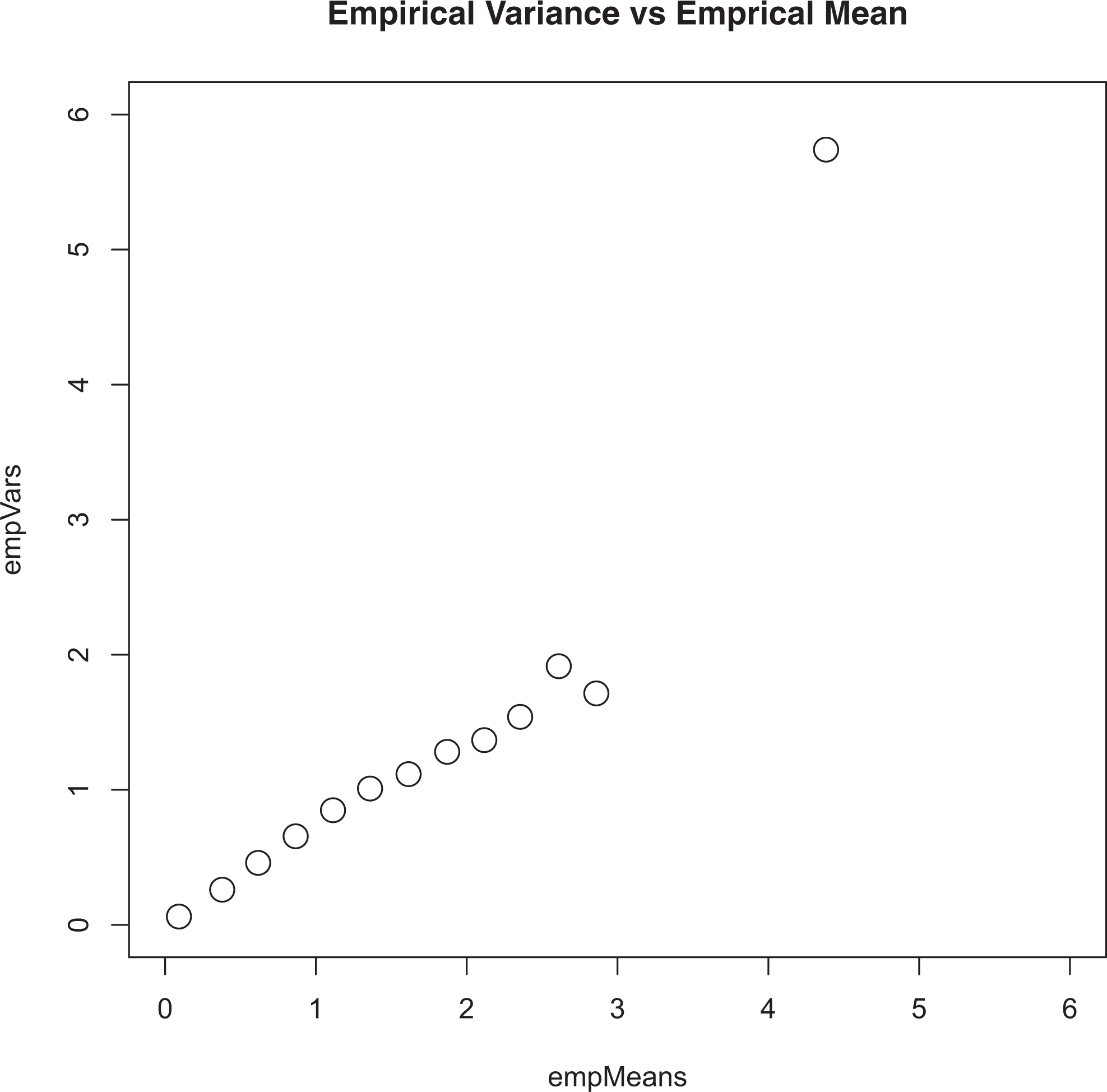
The results can be seen in Figure 1, wherein the linear trend (excepting the rightmost point, which constituted less than 2% of all total ${\hat{μ}}_{i j}$ ) signifies that the quasi-Poisson model fits relatively well. Recall that the parameter of the quasi-Poisson model was .724, which corresponds roughly to the slope of the best-fit line of the points below (except the last). This means that the variance of the actual observations is about 72% of what we would expect it to be under Poisson regression. Taking this into account impacts the standard errors of the quasi-Poisson regression coefficients but not their point estimates.

Figure 1.

Plot of the estimated means by the empirical variability about the means.

The results for the logistic model can be found in Table 4. Some important things to note about the logistic regression are that the probability of a penalty card decreases as Yellows.To.Give decreases or Suspension.Duration increases, as expected. For example, suppose a player who is two yellow cards away from a two-game suspension has a 10% probability (and hence 1/9 odds) of getting a penalty card in a given game. Were this player to have instead just one yellow card to give, this would multiply his odds of receiving card by $\exp (- 4.0109 + 2.8234) = .305$ , resulting in a 3% probability of getting a penalty card. Were this same player to have two yellows to give but face a potential one-game suspension, this would multiply his odds by $\exp (- 1.7461 + 2.8234) = 2.937$ , for a final probability of 25%. In addition, committing one more foul per game multiplies the odds of getting a penalty card by approximately exp(.8640) = 2.373. For a player with an underlying 10% probability of receiving a card, a 2.373-fold increase in his odds corresponds to a probability of 21%. The effect for playing at home is small but discernible. In our running scenario, playing at home versus away reduces a player’s probability of receiving a card from 10% to 8%. Having corrected for the point differential and many other possible lurking variables, it seems reasonable to attribute most of this modest reduction to referee rather than player behavior. Especially when considered in light of the existing literature on the topic, we feel that this finding provides evidence of a slight referee bias in favor of the home team.

Table 4.

Results for the Logistic Regression Model (Dependent Variable: Indicator of Whether Any Penalty Card Was Received).

Variable name	Estimate	SE	$\Pr (> \| z \|)$
Weeks.Until.Cutoff	−0.0713	.0089	.0000
Y1S1	−2.4330	.3321	.0000
Y2S1	−1.7461	.2281	.0000
Y1S2	−4.0109	.8291	.0000
Y2S2	−2.8234	.7418	.0001
Yellows.To.Give.Linear	0.6460	.0422	.0000
Suspension.Duration.Linear	−2.5246	.1661	.0000
Match.Differential	−0.0619	.0209	.0031
Total.Successful.Passes.All	−0.0077	.0030	.0108
Total.Fouls.Won	0.0405	.0457	.3750
Interceptions	0.0707	.0262	.0071
VenueHome	−0.2335	.0740	.0016
Blocked.Shots	0.1787	.0655	.0063
Unsuccessful.Dribbles	0.0630	.0498	.2061
Tackles.Won	−0.0260	.0395	.5116
Total.Clearances	0.0119	.0166	.4726
Challenge.Lost	0.0125	.0488	.7974
Duels.lost	0.0168	.0234	.4741
Duels.won	0.0013	.0242	.9556
Total.Fouls.Committed	0.8640	.0438	.0000

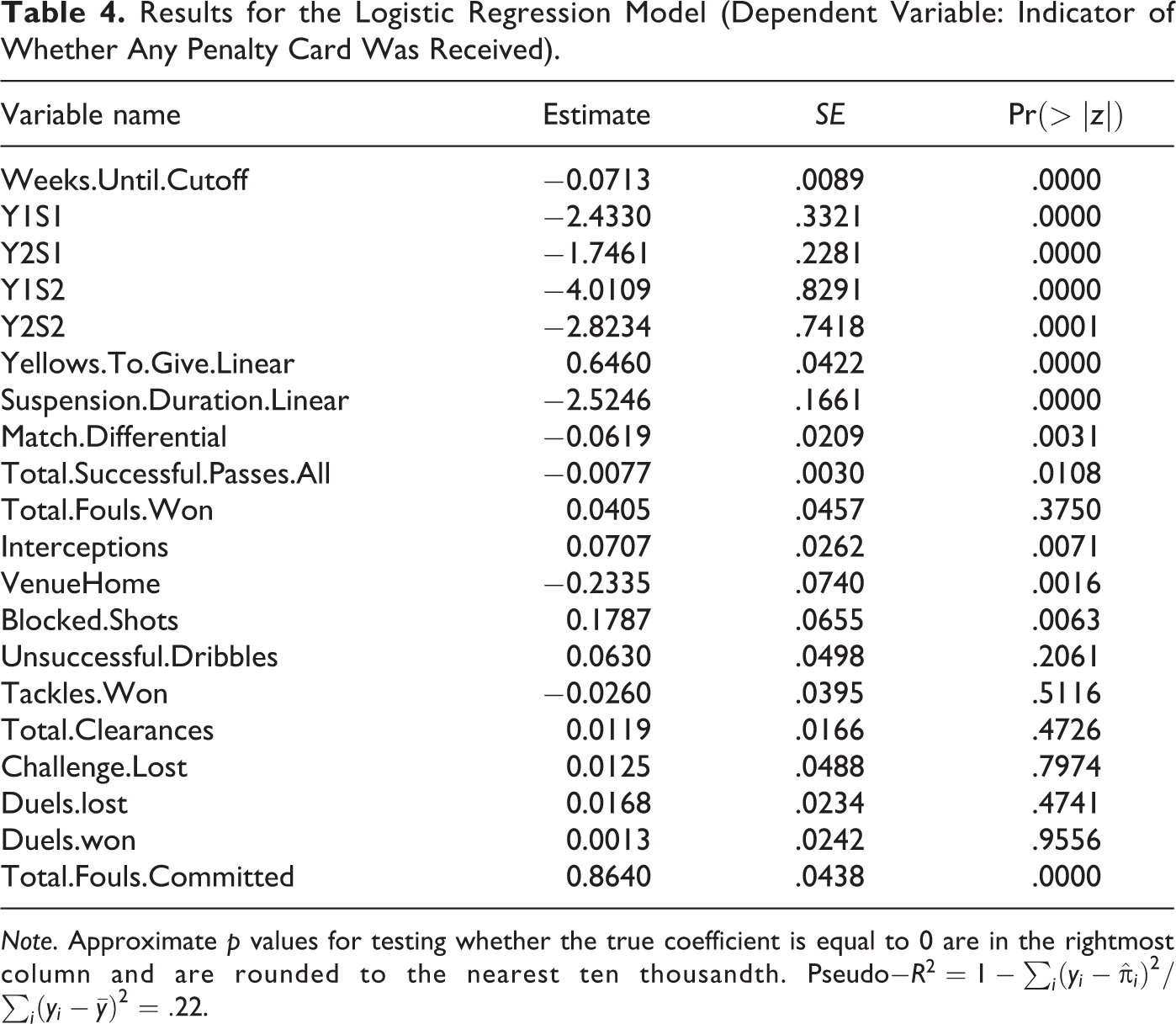
Note. Approximate p values for testing whether the true coefficient is equal to 0 are in the rightmost column and are rounded to the nearest ten thousandth. $Pseudo- R^{2} = 1 - \sum_{i} {(y_{i} - {\hat{π}}_{i})}^{2} / \sum_{i} {(y_{i} - \bar{y})}^{2} = .22$ .

Theoretical Model

The rule that suspends a player who has accumulated a certain number of yellow cards over the course of more than one game creates a dynamic problem for a player since a yellow card received early in the season affects the probability of being suspended later on. We analyze this dynamic problem using a quantitative theoretical model. We discuss what economic theory predicts about the evolution of the optimal level of aggressiveness over time and how it depends on some factors the player has control over and some he does not. We use standard dynamic programming techniques.

The state variable for the player is the number of yellow cards away from suspension. We denote it with y, and it can take values of $0, 1, 2, \dots, \bar{y}$ (in Premier League $\bar{y} = 5$ ). When y = 0, the player sits out that game. When y > 0, the player chooses his effort for the game. We denote the effort with x ≥ 0.

The effort has two effects. First, it affects the probability the player’s team wins, potentially increases the player’s market value, his happiness from playing well, and so on. All these factors are captured by a strictly increasing, strictly concave, current period payoff function w. Second, the more effort the player puts in, the higher his perceived aggressiveness tends to be. The perceived aggressiveness of the player is denoted with z, and we assume that z is the sum of the player’s actual effort x, and a random variable ε:

z \equiv x + ε, ε \sim N (0, σ^{2}) .

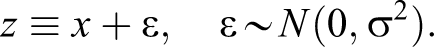
A player will get a yellow card if $z > \bar{z}$ . Such a specification captures a few interesting aspects. Ultimately, for a player to get a yellow card, a referee must call a foul and decide to give a yellow card. Whether this happens depends partially on the player’s behavior x and partially on a random component ε. The random component captures the referee’s personality, bias, ability to spot dangerous play, or being susceptible to diving—intentional falls by other players who pretend to be fouled.³ It can also capture the fact that sometimes a penalty card may be given even if a player was not trying to be particularly aggressive and that play may look/be more aggressive than intended.

Suppose a player starts a game at y yellow cards away from suspension. He chooses effort level x which yields current payoff w(x). If the realization of ε is such that $z > \bar{z}$ , then in the next game he will start at y − 1 cards away from suspension. When y = 0, the player is suspended, and his current period payoff is −κ, where κ is the utility cost of not being able to play. The first time a player is suspended, he sits out one game. For every suspension after that, the player sits out two games.

The dynamic programming problem of the player can be written as follows:

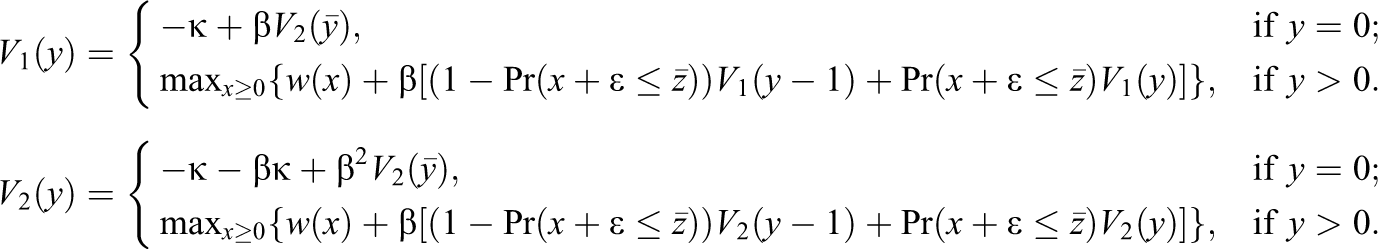
\begin{matrix} V_{1} (y) = {\begin{cases} - κ + β V_{2} (\bar{y}), & if y = 0; \\ \max_{x \geq 0} {w (x) + β [(1 - \Pr (x + ε \leq \bar{z})) V_{1} (y - 1) + \Pr (x + ε \leq \bar{z}) V_{1} (y)]}, & if y > 0. \end{cases} \\ V_{2} (y) = {\begin{cases} - κ - β κ + β^{2} V_{2} (\bar{y}), & if y = 0; \\ \max_{x \geq 0} {w (x) + β [(1 - \Pr (x + ε \leq \bar{z})) V_{2} (y - 1) + \Pr (x + ε \leq \bar{z}) V_{2} (y)]}, & if y > 0. \end{cases} \end{matrix}

where β is the discount factor, $ε \sim N (0, σ^{2})$ , $\bar{y} \in ℕ$ . We assume w(0) = 0, w′(0) > 0, w″ < 0, and there exists a unique x > 0 such that w′(x) = 0. These assumptions on w ensure that there is always a unique optimal level of effort in a single game, even if there are no suspension rules. The value function V_i, i = 1, 2, corresponds to the state when a player would potentially face a i-game suspension.

In order to simplify the analysis, we abstracted from the fact that the season ends and considered an infinite horizon problem. We also simplified the situation by assuming there is no three-game suspension, which dampens the estimated effect of suspension rules. Finally, we assume all players who have not received a one-game suspension remain eligible for it throughout the season; that is, we ignore the fact that for such players, on January 1, the suspension duration switches to 2 and there is an automatic increase in y. This simplification inflates the estimated effect of suspension rules. Relaxing these assumptions is an avenue for future research.

Characterization

At the beginning of the game, before realization of ε, the player chooses his effort level x. Let $x_{i}^{*} (y)$ denote the optimal level of effort x for a player who is y yellow cards away from being suspended for i game(s). For a given level of $y = 1, \dots, \bar{y}$ , the optimal levels of effort $x_{1}^{*}$ and $x_{2}^{*}$ must satisfy the following first-order conditions:

w' (x_{1}^{*}) = \frac{β}{σ} ϕ (\frac{\bar{z} - x_{1}^{*}}{σ}) \cdot [V_{1} (y) - V_{1} (y - 1)],

and

w' (x_{2}^{*}) = \frac{β}{σ} ϕ (\frac{\bar{z} - x_{2}^{*}}{σ}) \cdot [V_{2} (y) - V_{2} (y - 1)],

where φ denotes the probability distribution function of a standard normal distribution. Since both V₁ and V₂ are endogenous objects, we do not provide analytical results. Instead, we characterize the model numerically. We solve the model by iterating on the value function.

Numerical Analysis

In this section, we analyze how the expected number of fouls committed depends on various model parameters. We also analyze how it evolves as the state variable y changes (which we analyze in the data).

Functional forms, parameter values, and calibration

Since our model serves illustrative purposes only, we provide an ad hoc parameterization with parameters that we are able (with a few exceptions) to calibrate to match Premier League statistics. The period payoff function w(x) is assumed to be quadratic: $w (x) = a x^{2} + b x$ . We set a = −1, and we calibrate b = 6, so the optimal level of effort without suspension rules is x* = 3. We chose this target, because it is a little above the average number of fouls committed per game and thus represents how aggressive players might be in the absence of suspension rules. While not perfect, the number of fouls called on a player is a reasonable measure of his effort. The number of yellow cards the player needs to accumulate to be suspended is set to $\bar{y} = 5$ (the Premier League threshold). The variance of the random shock is σ² = 1, and the threshold value for z ≡ x + ε that yields a yellow card is set to $\bar{z} = 2$ . While $\bar{z}$ is arbitrary (we have no way to learn it from our data), we want to point out the scale we choose is not important. Specifically, if we set the standard deviation of the random shock to be σ_new and set ${\bar{z}}_{new} = 2 σ_{new}$ , then taking $a_{new} = a / σ_{new}^{2}$ and $b_{new} = b / σ_{new}$ (so that $x_{new}^{*} = 3 σ_{new}$ ) would yield identical results.

The utility cost κ and the discount factor β are jointly calibrated to match the effort profile of a player before a one-game suspension. Specifically, we target two numbers from Table 3—expected numbers of fouls for players at one and at five yellow cards away from a one-game suspension, relative to the player at three cards away from a one-game suspension: 0.76 and 1.14, respectively. Our calibrated values are β = .86 and κ = 13.79. The model fit is presented in Table 5. Overall, our very stylized model matches the empirical estimates remarkably well, with exception of the cases of four and five yellow cards away from a two-game suspension, where we overshoot the expected number of fouls.

Table 5.

Model Fit.

	Suspension.Duration
	One Game		Two Games
Yellows.To.Give	Theoretical Model	Regression Model	Theoretical Model	Regression Model
1	0.76^a	0.76	0.54	.57
2	0.89	0.86	0.71	.74
3	1.00^a	1.00	0.85	.77
4	1.08	1.07	0.96	.82
5	1.14^a	1.14	1.06	.88

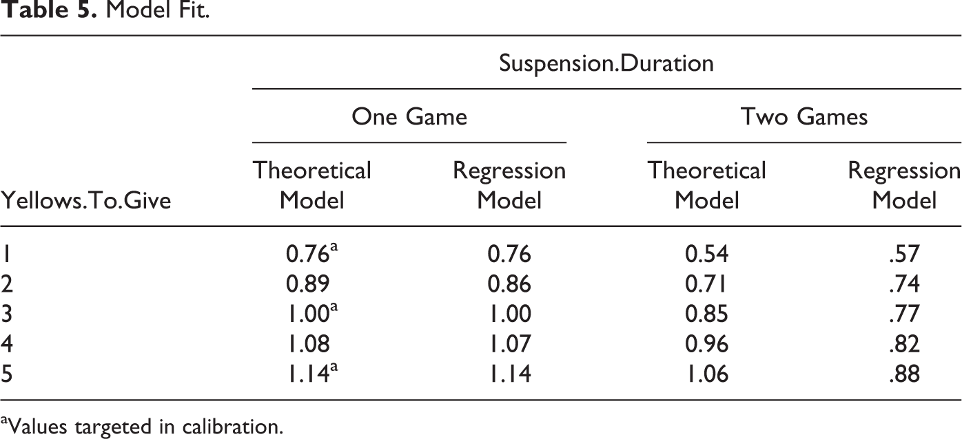
^aValues targeted in calibration.

Fouling as a function of number of yellow cards

We first show that our model’s predictions are consistent with the empirical estimates presented in the “Regression Models” section. Figure 2 shows how expected number of fouls evolves as the player accumulates more yellow cards. In that figure, we normalized the expected number of fouls in the very first game of the season to be one. The blue line shows how this number evolves as the player gets closer to a one-game suspension. The dashed red line shows the expected number of fouls for a player facing a possible two-game suspension. While the model was parameterized to match the end point and the midpoint of the blue line, the red dashed line is an endogenous outcome of the model. 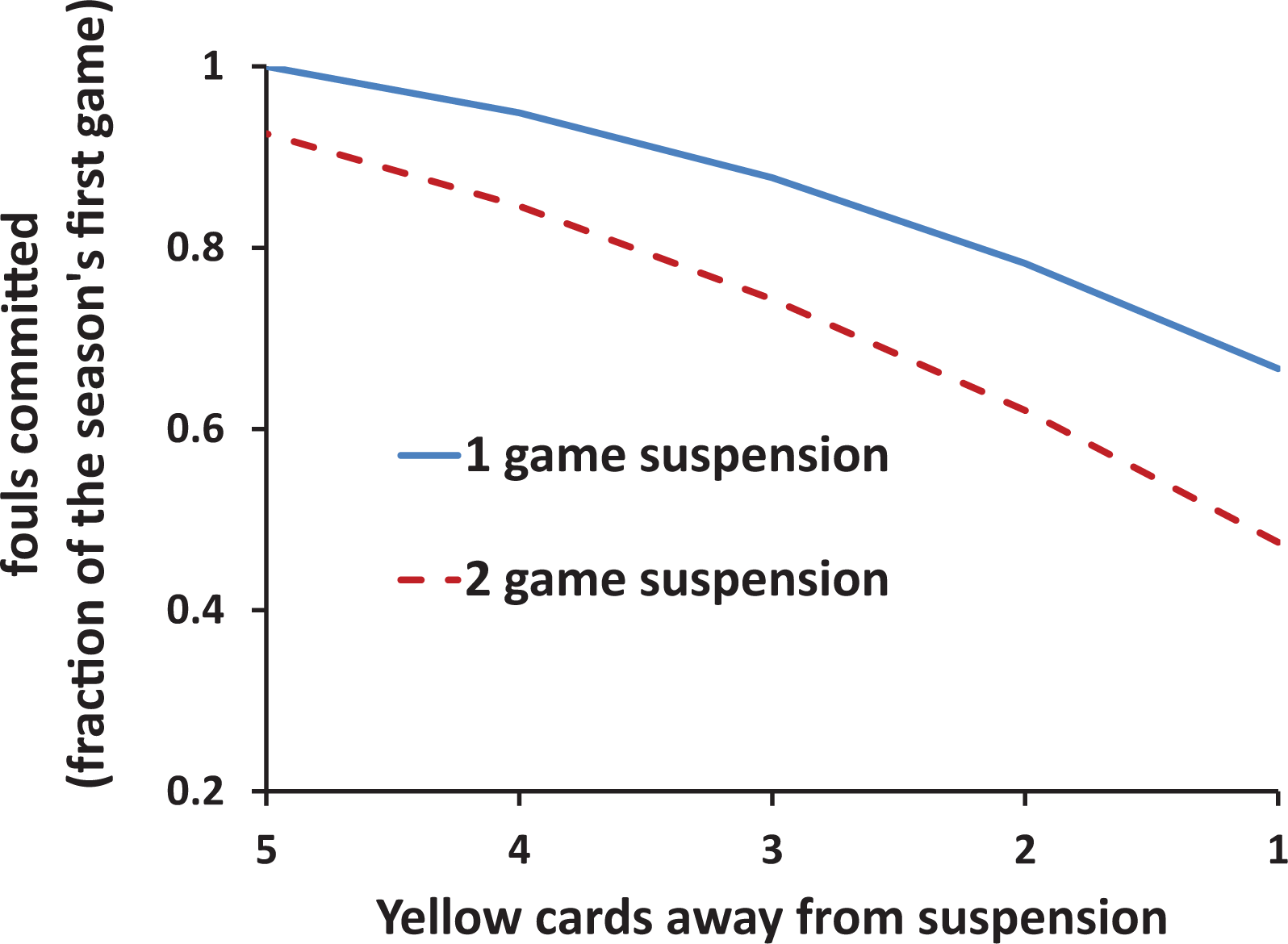If the player is only one card away from a two-game suspension, he fouls less by 53% relative to his very first game of the season $(.53 = 1 - (.54 / 1.14))$ . If he is two cards away, he fouls less by 38%. The empirical estimates were 50% and 35%, respectively (these can be computed using estimates in Table 3).

Figure 2.

Fouls drop as we get closer to suspension.

Fouling as a function of parameters of interest

Some important model parameters were chosen arbitrarily, because we did not have data to properly calibrate them. We now analyze how the model’s predictions depend on some parameters of interest, namely, $\bar{z}$ , σ², β, and $\bar{y}$ . For each parameter, we present a figure with three curves that describe the parameter’s effect on the number of fouls committed. The dashed blue curve gives the number of fouls committed when a player is one yellow card away from suspension (when y = 1) divided by x*, the number of fouls committed under no suspension rules. The dot-dashed red curve gives the number of fouls committed on the first game of the season (when $y = \bar{y}$ ) divided by x*. (In the plots, we refer to this division by x* as “fraction of the optimal.”) The solid black curve gives the ratio of these, the number of fouls committed when a player is one yellow card away from suspension divided by the number of fouls committed on the first game of the season. The calibration mentioned earlier forces the black curve to pass through the point 0.67 (0.76/1.14 from Table 3) at the benchmark value of each parameter.

We start with $\bar{z}$ , the level of perceived aggressiveness that results in a yellow card. Figure 3 shows how $\bar{z}$ affects the player’s aggressiveness. The effect is nonmonotone. In order to see why this is the case, note that the decrease in $\bar{z}$ is essentially an exogenous (to the player) increase in the probability of getting a yellow card. A slight decrease in $\bar{z}$ means that, for a given level of effort x, a player is more likely to get a yellow card and sit out the next game. The player then can affect the outcome by playing less aggressively. However, a sufficiently low value of $\bar{z}$ means a very high probability of getting a yellow card regardless of the player’s behavior: He will be punished even if he does not play aggressively. In this case, the player has incentive to play essentially as aggressively as w permits. When $\bar{z}$ is large, the player also has incentive to play aggressively, since there is little worry that he will be booked.

Figure 3.

Effect of $\bar{z}$ on fouls committed.

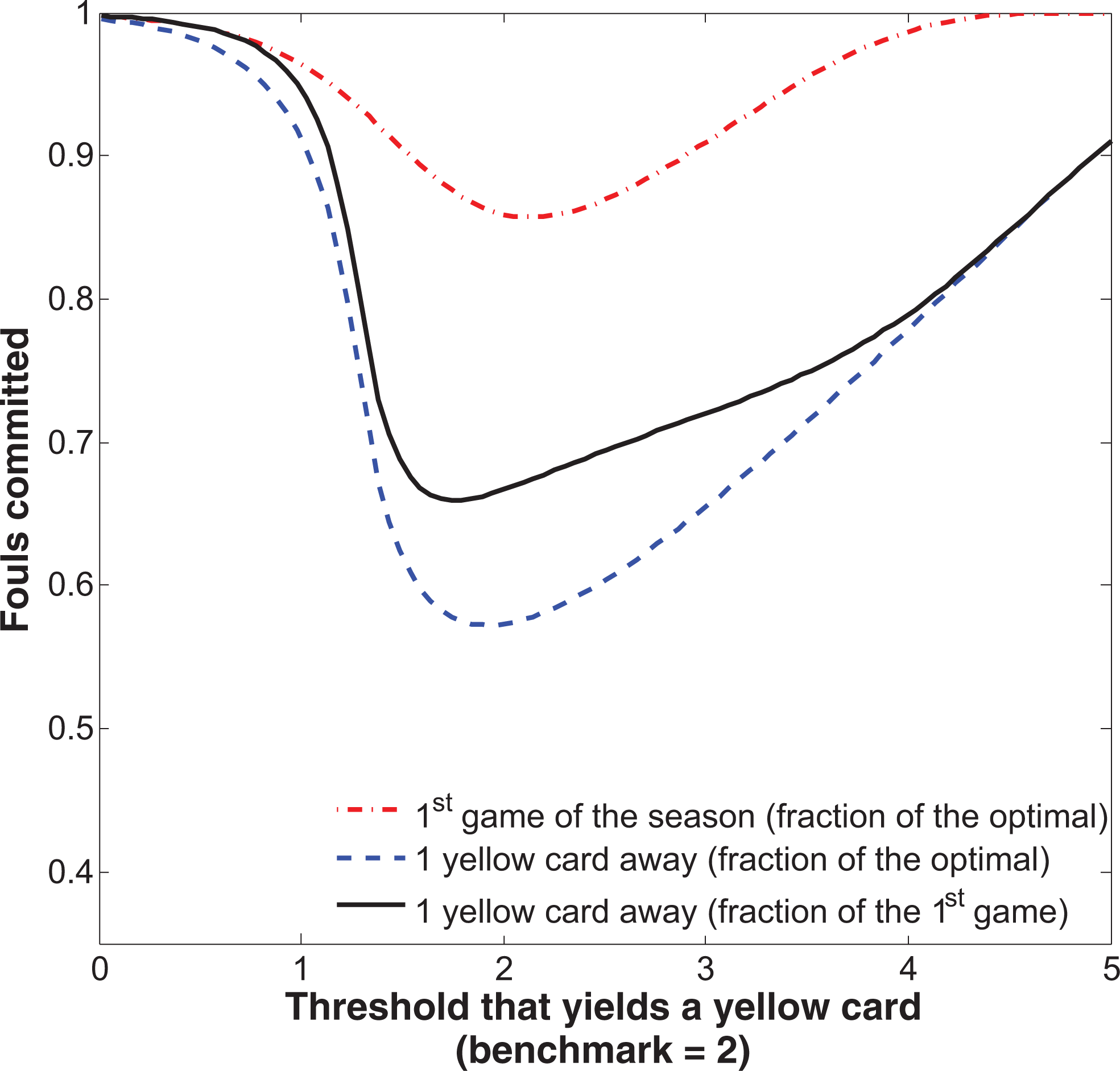
Figure 4 shows the effect of σ²—the variance of the random element of “booking,” ε. As the variance increases, player aggressiveness eventually increases. In the limit, as the variance tends to infinity, the probability of getting booked depends less and less on the player’s behavior. Accordingly, he will foul as much as w permits. The effect of a decrease in σ² is more complex. As σ² declines, the number of fouls first drops, and then starts to increase. The initial drop is intuitive: Smaller variance of the random component means that more aggressive play is more likely to be detected, while play that is not aggressive is less likely to be mistakenly punished with a yellow card.

Figure 4.

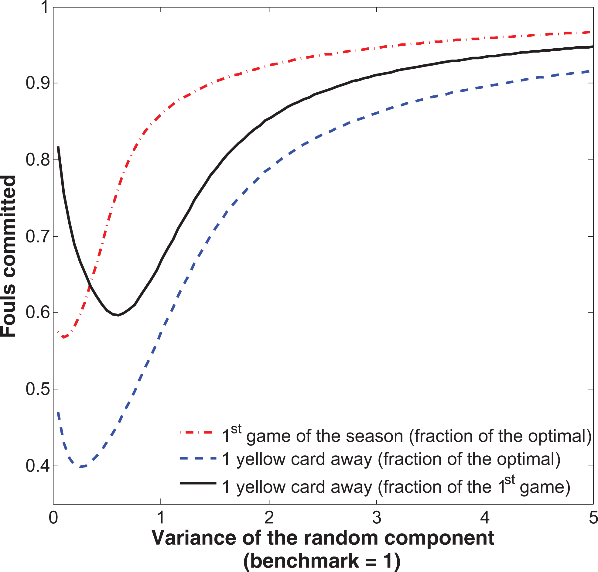
Effect of σ² on fouls committed.

The subsequent rise is more subtle. For a given level of σ, the player faces a certain probability of not getting a yellow card. As σ declines, that probability gets smaller, inducing him to play less aggressively (i.e., lowering x closer to $\bar{z}$ ). The marginal effect of x on the probability of getting a yellow card is $(1 / σ) \cdot ϕ (\bar{z} - x^{*} (y) / σ)$ (see the first-order conditions [Equations 1 and 2]). That effect is going to 0 as σ → 0, because (1/σ) → ∞ at a slower rate than $ϕ ((\bar{z} - x^{*} (y)) / σ) \to 0$ . The marginal cost of playing less aggressively is w′(x). At some level of σ, the marginal benefit of fouling less (proportional to the reduction in the probability of getting a yellow card) is not sufficient to outweigh the marginal cost, and thus as σ → 0 we observe an increase in the number of fouls committed.

Figure 5 shows the impact of the discount factor β on fouls committed. Of course, when the discount factor β = 0, players do not care about future games, and the effort is chosen so as to maximize w. Next, let’s consider the effect of an increase in β. For a player in the first game of the season, quite understandably, he tends to foul less as he values his future more (dot-dashed red curve). What is much more interesting is how increasing β impacts a player who is one card away from suspension (dashed blue curve). At first, the slope is negative, for the same reason that the dot-dashed red curve has negative slope. But then, around β = .6, the player starts to foul more. 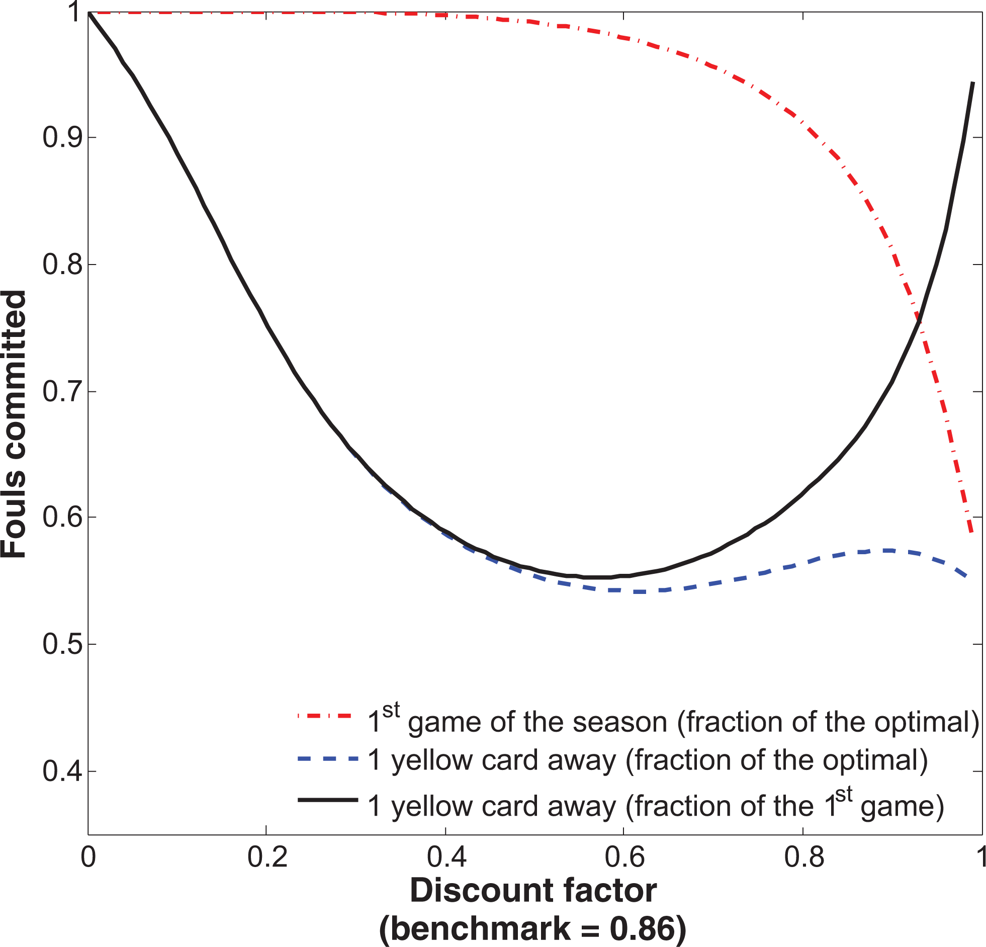We believe this is because the player values his future enough that the benefit of getting y reset to $\bar{y}$ is beginning to outweigh the cost of a one-game suspension. It is not that he is trying to get a penalty card,⁴ he just is content to play with an effort closer to x*.

Figure 5.

Effect of β on fouls committed.

The careful reader will notice that the dashed blue curve goes down again once β > .9. We attribute this to the fact that for players who are particularly forward thinking, not only does the benefit of being able to play more aggressively in future games matter, but the cost of sitting out future games matters as well. This type of behavior was suggested at in the discussion of incentives faced by players in this environment (see “Incentives Caused by Suspension Rules” subsection). It is exciting to see it borne out in the dynamic model.

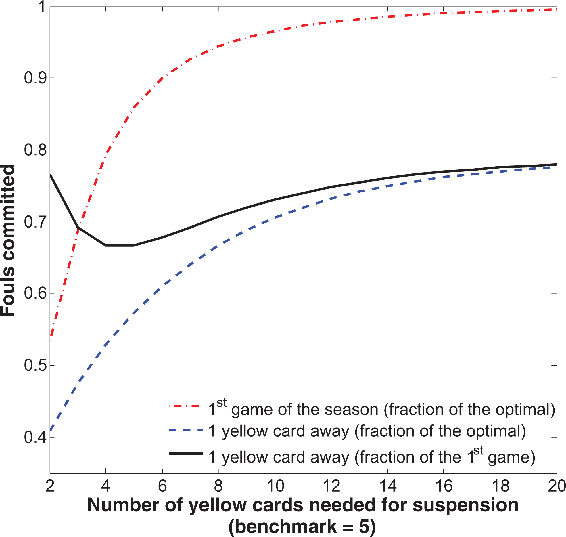
Figure 6 shows the effect of $\bar{y}$ on the number of fouls committed. Not surprisingly, for a player with $y = \bar{y}$ , increasing $\bar{y}$ increases the number of fouls committed (dot-dashed red curve). When y = 1, the dashed blue curve is also monotone increasing, but it is bounded above by the dot-dashed red curve. When $y = \bar{y} = 1$ (not shown), the two curves intersect because their definitions coincide. These constraints force the solid black line to be U shaped.

Figure 6.

Effect of $\bar{y}$ on fouls committed.

Impact of Suspension Rules on Fouling

Finally, we can use the model to evaluate the impact of suspension rules on fouling. The advantage of using a structural model is that we can run a counterfactual experiment by removing the suspension rule and simulating the average number of fouls players commit during the whole season. To do so, we run the following simulation. We draw 11 × 20 × 38 values of ε (11 players that start a game in 20 different teams, multiplied by 38 games played by each team). Then, for each player we can track the evolution of his yellow cards, and compute his effort using the solution to the dynamic programming problem. When the player sits out, we assume his replacement only cares about the current game, so x* = −b/2a. The rationale is that the replacement player plays so infrequently, he will never accumulate five yellow cards. We run the simulation 100 times and calculate the average number of fouls per player per game, and compare it to x* = −b/2a, which would be the number of fouls per game had the suspension rule not been in place.

Notice, that by using the structural model (rather than econometric estimates) in our counterfactual analysis, we take into account one very important factor: Players foul less even in the very early stages, because they fear getting closer to the situation when y = 1. This effect is a known feature of the three-strikes laws intended to curb criminal behavior (Shepherd, 2002) and soccer players should also fear getting even the first strike. In other words, our econometric estimates were obtained in the environment with suspension rules in place: We cannot use our data to estimate how aggressively players would play in the beginning of the season, had there not been the suspension rule. In macroeconomic literature, this is often referred to as the Lucas’ (1976) critique: In general, the econometric estimates of relationships between different variables change when a policy changes.

Since our parameterization in this article was somewhat arbitrary, we perform this counterfactual experiment for a variety of different parameter values. That way we evaluate what factors (in theory) make the suspension rules more effective in reducing player aggressiveness. The results are presented in Table 6.

Table 6.

Quantitative Impact of Suspension Rules on Average Number of Fouls—Model Simulations.

	Sensitivity Analysis
Benchmark	β		$\bar{y}$		$\bar{z}$		σ²
	0.95	0.65	10	3	3	1	2	0.25	0.001
0.66	0.62	0.72	0.83	0.54	0.77	0.93	0.84	0.48	1.00
(0.002)	(0.001)	(0.003)	(0.002)	(0.003)	(0.003)	(0.000)	(0.001)	(0.002)	(0.000)

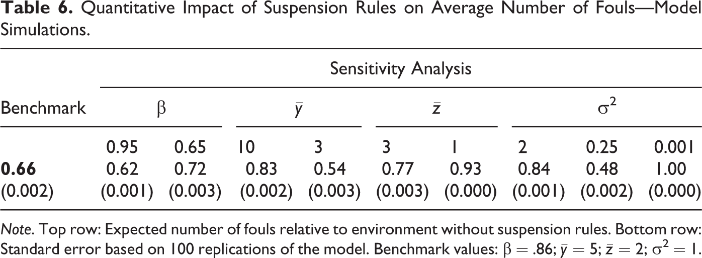
Note. Top row: Expected number of fouls relative to environment without suspension rules. Bottom row: Standard error based on 100 replications of the model. Benchmark values: β = .86; $\bar{y} = 5$ ; $\bar{z} = 2$ ; σ² = 1.

Our results suggest the existence of suspension rules can have a large impact on the level of aggressiveness. The average number of fouls, relative to an environment where no suspensions ever take place, is lower by 34%. That drop would have been 46%, should suspension take place after three yellow cards were accumulated.

It is also interesting to see how the random component affects the effectiveness of suspension rules. First, consider the effect of $\bar{z}$ , which measures how lenient the referees are during the game. Both very low levels of $\bar{z}$ (harsh referees) and very high levels of $\bar{z}$ (lenient referees) reduce the effectiveness of suspension rules. The intuition behind this result is identical to the intuition behind Figure 3: In both cases, the punishment becomes less dependent on player’s behavior. When referees are lenient, players know they can get away with aggressive play, so they play more aggressively. When referees are harsh, players believe even a minimal amount of effort will be considered too aggressive, so they might as well put forth a very high effort since the punishment will likely be the same.

Finally, we can also see that a small amount of randomness in booking is necessary for the suspension rules to impact player behavior. Increasing σ² from 1 to 2 reduces the effectiveness of suspension rules. Similarly, reducing it from 1 to 0.25 makes the suspension rules more effective. However, when σ² becomes very small, the impact of suspension rules on number of fouls becomes smaller and disappears in the limit as σ² → 0. We find this to be potentially a very interesting result, posing questions about the effectiveness of the certainty of punishment (Nagin, 2013).

The estimates in Table 6 represent a first pass at evaluating the impact of suspension rules on aggressive behavior. Many features of the real world are not accounted for in our simple model. First, we are not able (with our data set) to pin down the value of $\bar{z}$ , the parameter that determines when a player would get a yellow card. Second, we do not account for players’ observable and unobservable heterogeneity (e.g., defenders typically foul more, some play more aggressively than others, etc.). In addition, some players are more important for their teams, and they may be especially cautious when they get closer to the suspension. Despite these limitations, we believe our analysis demonstrates that suspension rules do have substantial impact on player aggressiveness.

Conclusion

The main goals of punishment rules in soccer are to protect the health of players and maintain the integrity of the game. Yellow cards were introduced in the 1960s and tested during the 1970 World Cup. In late 1980s and early 1990s, different leagues and tournaments introduced additional punishment: suspension for one or more games of players who had accumulated too many yellow cards. Using Premier League data from the 2011-2012 season, we found that additional punishment matters: Players foul less.

In the theoretical section, we provided some guidance for showing what factors may have the biggest impact on player aggressiveness. We think this is a good first step toward the design of optimal punishment rules. An optimal punishment rule is different from the rule that completely removes potentially dangerous play, however.⁵ Things such as slide tackles or accidental collisions between players are intrinsic parts of soccer: They provide enjoyment for fans that turns into income for players and sponsors. When thinking about optimal punishment rules, one must weigh the benefits of such enjoyment, and the costs resulting from possible injuries. This requires a very careful and thorough analysis that we think is a fascinating avenue for further research.

Our analysis can be fine-tuned by using a more refined data set which would allow for the estimation of the threshold level of aggressiveness that results in a yellow card. Such a data set would have to include measures of the actual level of aggressiveness (possibly based on postgame evaluation by experts) combined with data on which behaviors resulted in a penalty card. It would also need to distinguish between penalty cards awarded for aggressive play and those awarded for other types of unwanted behavior.

Footnotes

Appendix

Declaration of Conflicting Interests

The author(s) declared no potential conflicts of interest with respect to the research, authorship, and/or publication of this article.

Funding

The author(s) received no financial support for the research, authorship, and/or publication of this article.

Notes

References

Agresti

(2002). Categorical data analysis. New York, NY: Wiley.

Bar-Eli

Tenenbaum

Geister

(2006). Consequence of players’ dismissal in professional soccer: A crisis-related analysis of group-size effects. Journal of Sport Sciences, 24, 1083–1094.

Becker

(1968). Crime and punishment: An economic approach. Journal of Political Economy, 76, 169–217.

Bime. (2012). Bime and the MCFC Analytics Project with Opta. Retrieved January 13, 2016, from http://blog.bimeanalytics.com/english/bime-and-the-mcfc-analytics-project-with-opta

Brown

(2012). Testing Michel Owen: The alleged diving culture of “Players Coming From South America, Italy and Spain. Retrieved January 13, 2016, from https://harvardsportsanalysis.wordpress.com/2012/11/13/the-alleged-diving-culture-of-players-coming-from-south-america-italy-and-spain-testing-michael-owen/

Dawson

Dobson

Goddard

Wilson

(2007). Are football referees really biased and inconsistent?: Evidence on the incidence of disciplinary sanction in the English Premier League. Journal of the Royal Statistical Society—Series A, 170, 231–250.

del Corral

Prieto-Rodriguez

Simmons

(2010). The effect of incentives on sabotage: The case of Spanish football. Journal of the American Statistical Association, 11, 243–260.

Dobson

Goddard

Staehler

(2014). Tullock on the football pitch. Applied Economics and Finance, 1, 71–76.

Garicano

Palacios-Huerta

(2005). Sabotage in tournaments: Making the beautiful game a bit less beautiful (CEPR discussion papers 5231, C.E.P.R. discussion papers). London: Centre for Economic Policy Research Location.

10.

Garicano

Palcios-Huerta

Predergast

(2005). Favoritism under social pressure. The Review of Economics and Statistics, 87, 208–216.

11.

Greenwood

Rydell

Abrahamse

Caulkins

Chiesa

Model

Klein

(1994). Three strikes and you’re out: Estimated benefits and costs of California’s new mandatory-sentencing law (Technical Report MR-509-RC). Santa Monica, CA: RAND Corporation.

12.

Helland

Tabarrok

(2007). Does three strikes deter? A nonparametric estimation. The Journal of Human Resources, 42, 309–330.

13.

Kessler

Levitt

S. D.

(1999). Using sentence enhancements to distinguish between deterrence and incapacitation. The Journal of Law and Economics, 42, 343–364.

14.

Lucas

(1976). Econometric policy evaluation: A critique. Carnegie-Rochester Conference Series on Public Policy, 1, 19–46.

15.

McCormick

R. E.

Tollison

R. D.

(1984). Crime on the court. Journal of Political Economy, 92, 223–235.

16.

Morgulev

Azar

O. H.

Lidor

Sabag

Bar-Eli

(2014). Deception and decision making in professional basketball: Is it beneficial to flop? Journal of Economic Behavior & Organization, 102, 108–118.

17.

Nagin

(2013). Deterrence: A review of the evidence by a criminologist for economists. Annual Review of Economics, 5, 83–105.

18.

Nevill

Balmer

Williams

(2002). The influence of crowd noise and experience upon refereeing decisions in football. Psychology of Sport and Exercise, 3, 261–272.

19.

Opta. (2012). Opta’s event definitions. Retrieved January 13, 2016, from http://optasports.com/news-area/blog-optas-event-definitions.aspx

20.

Ramineni

(2012). MCFC Analytics data—The story so far. Retrieved January 13, 2016, from http://analysefootball.com/2012/09/03/mcfc-analytics-data-the-story-so-far/

21.

Ridder

Cramer

J. S.

Hopstaken

(1994). Down to ten: Estimating the effect of a red card in soccer. Journal of the American Statistical Association, 89, 1124–1127.

22.

Shepherd

(2002). Fear of the first strike: The full deterrent effect of California’s two and three-strikes legislation. Journal of Legal Studies, 31, 159–201.

23.

Snyder

J. A. L.

(2013). What actually wins soccer matches: Prediction of the 2011–2012 premier league for fun and profit (Master’s thesis). University of Washington, DC. Advised by Robert Schapire.

24.

Stride

Patterson

Thomas

(2011, 9 24). Cheating in soccer: Team culture, player behaviour or just a question of circumstance? New England Symposium on Statistics in Sports, Harvard University, Cambridge, MA. Retrieved from http://www.nessis.org/nessis11.html

25.

Sutter

Kocher

(2004). Favoritism of agents—The case of referees’ home bias. Journal of Economic Psychology, 25, 461–469.

26.

Tella

R. D.

Schargrodsky

(2004). Do police reduce crime? Estimates using the allocation of police forces after a terrorist attack. American Economic Review, 94, 115–133.

27.

Vecer

Kopriva

Ichiba

(2009). Estimating the effect of the red card in soccer—When to commit an offense in exchange for preventing a goal opportunity. Journal of Quantitative Analysis in Sports, 5, 1–20.

28.

Ver Hoef

Boveng

(2007). Quasi-Poisson vs. negative binomial regression: How should we model overdispersed count data. Ecology, 88, 2766–2772.

29.

Zimring

Kamin

Hawkins

(1999). Crime and punishment in California: The impact of three strikes and you’re out. Berkeley, CA: Institute of Government Studies Press, University of California.