
Abstract
This article examines the effects of team composition on the performance of European football (soccer) teams. The scorelines of 1,822 matches involving 98 first-tier teams were analyzed in terms of the overall ability of the teams and the spread of player abilities (heterogeneity) within them. As expected, total team ability has a beneficial effect on performance; the number of goals a team scores is positively related to its own ability and negatively related to the ability of its opponents. Team heterogeneity on the other hand has both beneficial and detrimental effects on performance. Heterogeneous teams score more goals than homogeneous teams, but they also concede more goals. As the effect of heterogeneity on goals conceded is greater than its effect on goals scored, the net effect of heterogeneity is to depress overall performance. The results are discussed in terms of Steiner’s framework of group dynamics.
Team working is a widespread method of organizing labor. Many companies rely on teams to accomplish a variety of productive tasks, and the problem of optimizing team productivity has attracted the attention of both labor force economists and organizational psychologists. Team productivity is obviously dependent on the average ability or productivity of its members and teams formed from high performing individuals outperform teams of low performers. However, it has long been known that because of intrateam processes, the relationship between team productivity and the productivity or ability of its members is not necessarily a strictly additive one. For example, social loafing, the tendency for individuals to expend less effort when working collectively than when working individually (Karau & Williams, 1993; Ringelmann, 1913), can cause a loss of efficiency. Conversely, the Kohler (1926) effect, where performance gains are seen in weaker individuals who are striving to keep up, can enhance team efficiency.
The question addressed in this article concerns the optimum mix of abilities for a football team. Let us suppose for a moment that the cost of a football player reflects his ability. Now given a fixed budget for recruiting players and paying their wages, how should a football club deploy its available funds to construct the most effective team? One strategy is to create a heterogeneous team; here the club spends a large amount of money to recruit a small number of (expensive) high ability players and spends the rest on a mediocre supporting cast. An alternative strategy maximizes homogeneity; instead of recruiting any outstanding individuals, the available funds are spread as evenly as possible among the players so as to avoid any areas of weakness.
Some guidance as to the relative merits of these strategies can be found in the psychological and economic literature. Theoreticians in both domains have argued that the effects of heterogeneity on team performance are not the same in all situations but depend strongly on task characteristics. In Steiner’s (1972) theory of group dynamics, performance on an additive task depends on the sum total of the team member’s abilities. Examples of additive tasks include collaborating to lift a heavy weight or running a relay race. Steiner also distinguishes between conjunctive and disjunctive tasks. In conjunctive tasks, successful team performance is dependent on the completion of a joint action. Here, heterogeneity is detrimental to team performance, because if overall ability is held constant, a heterogeneous team must contain a weakest member who limits the overall performance of the team. In disjunctive tasks, team performance is determined by the output of the best performing member (an example is maximizing a nation’s tally of Olympic gold medals). In this case, heterogeneity is beneficial because a heterogeneous team must contain one or more stronger performers than a homogeneous team of the same overall ability. In economics (e.g., Prat, 2002), the actions that constitute a conjunctive task are said to be mutually reinforcing and positive complements of each other; disjunctive tasks on the other hand consist of actions that are substitutes for, or negative complements of, each other. Prat used lattice theory to demonstrate theoretically that with positive complementarities, performance is optimized when the team is homogeneous and with negative complementarities, performance is optimized when the team is heterogeneous.
Since Lazear (1995), economists in the subfield of personnel economics have long sought to understand the relationships between team heterogeneity and productivity in organizations. Much of this research has focused on the effects of pay disparity within teams.
The football industry is well-known for its wide wage disparities. For example, in the 2015-2016 season, the average weekly wage of the first-team squad at Chelsea Football Club (a team in the English Premier League) was £89,391. The five lowest earners averaged £26,000 and the five highest £162,000. This order of discrepancy is typical of many clubs. Cohesion theory (e.g., Levine, 1991) predicts that such disparities would prove detrimental to performance because they deflate group unity.
Several studies (e.g., Coates, Frick, & Jewell, 2016; Depken, 2000) have indeed found that wage disparities in professional sports teams are associated with reduced team performance. Frick, Prinz, and Winkelmann (2003) however presented a more nuanced view. These authors found that the effect of wage disparity was detrimental for football and baseball and positive for hockey and basketball and argued that the effects of wage disparity wage were moderated by team size.
A second source of heterogeneity in modern sports teams is culture. Kahane, Longley, and Simmons (2013) found a U-shaped relationship between team heterogeneity and performance in the National Hockey League. Teams with more foreign players performed better—provided they hailed from the same country. When the foreign players came from a variety of countries, the costs of cultural and linguistic integration began to offset the gains from diversity.
Turning to the research on ability, Hamilton, Nickerson, and Owan (2003, 2012) considered the effects of mixing ability levels in a team and measured the impact of member heterogeneity on productivity. They argued that where a task requires technical skill, heterogeneous teams should demonstrate productivity gains through a process of in-group learning, whereby less skilled or experienced employees gain expertise by working alongside more able colleagues. Furthermore, depending on the structure of incentivization, introducing heterogeneity by including highly productive workers in a team can produce elevated production norms in the team and thus higher overall output. As predicted, the authors found empirical evidence for increased productivity in heterogeneous teams among workers in a garment factory. When average worker productivity was controlled, teams formed from individuals with disparate individual productivities had higher outputs than their more homogeneous counterparts.
Hoogendoorn, Parker, and Praag (2012) examined the effects of team heterogeneity in a business simulation task. Teams of business school students constructed with either more or less diversity in cognitive ability. Controlling for overall team ability, an inverse-U relationship was found where increasing heterogeneity was associated with better performance up to a maximum, after which further increases in heterogeneity led to a drop-off.
Although various dimensions of diversity clearly influence the performance of teams, the focus of the present study is ability. In professional sports teams, ability and pay are closely related, but ability is more proximate to performance than pay. Despite this, only a few studies have directly investigated how the ability mix influences the performance of sports teams.
Anderson and Sally (2013) examined the effects of heterogeneity on the performance of soccer teams over one season of first-tier European domestic football. They regressed measures of player ability for the most able player (the “strongest link”) and 11th-ranked player (the “weakest link”) in each team against the average points earned per match. They concluded that performance levels were primarily dominated by the strength of the weakest link. However, the regression model omitted the ability of the remaining nine players and seems therefore underspecified.
In a more detailed study of European football, Franck and Nüesch (2010) examined the effects of different mixes of ability at two levels of analysis. The first level examined aggregate performance over a complete season. The heterogeneity of the squad was measured at the start of the season, and performance was measured by league position at the end of the season. Holding average ability, unobserved team heterogeneity, and other confounding variables constant, increasing heterogeneity was associated with improved performance. Franck and Nüesch attributed this finding partly to the effects of in-group learning and partly to the substitutive nature of the team selection process, whereby the more talented players in the squad get picked to play more often, so that for a given level of overall ability, a stronger team can be selected from a heterogeneous squad than from a homogeneous one.
In a conceptually similar study, Papps, Bryson, and Gomez (2011) examined the effects of team composition on the batting and pitching performance of baseball teams. The overall talent and heterogeneity of teams were assessed at the start of the season, and performance was measured by the total number of matches won. In contrast to Franck and Nüesch, however, these authors found that teams with a middling degree of heterogeneity among their members performed better than teams that were either more homogeneous or more diverse. Papps et al. attributed the positive element of the heterogeneity performance relationship partly to in-group skill transfers and partly to sports-specific factors such as an increased frequency of sacrifice plays. The negative element of the relationship was attributed entirely to sports-specific factors; for example, large differences in pitching ability would allow opposing teams to exploit weaker pitchers by matching opposing hitting line-ups more easily, while a batting line-up consisting of a few very talented hitters preceded and followed by poor hitters could be countered by throwing the least favorable pitches to the best hitters.
Franck and Nüesch’s (2010) second study examined how the heterogeneity of the team on the field influenced the results of individual matches. In this case, performance, which was measured by goal difference (goals scored by the target team minus goals scored by the opposition), showed a negative relationship with heterogeneity. The authors suggested that heterogeneous teams are disadvantaged because they contain weak players, which because of the complementarity between players and the collaborative requirements of the game depresses the performance of the whole team.
In this article, I explore the effects of heterogeneity at the match level in football, but in contrast to Franck and Nüesch, the statistical model I use permits the effects of heterogeneity on attack and defense to be estimated separately. This sheds further light on the effects of team composition on sporting performance.
Material and Method
Data Sources
Player abilities were taken from the Castrol Edge player ranking website (http://www.castrolfootball.com/rankings/rankings; Retrieved June 13, 2013). Team compositions were taken from an OptaSports data set of 1,822 matches which took place in the English Premiership, French Ligue 1, German Bundesliga, Spanish La Liga, and Italian Serie A in the 2012-2013 season and which involved 2,623 players in 98 teams. The OptaSports data set identified the players (including substitutes) in each match and the number of minutes they played. It also contained the number of successful and unsuccessful pitch actions of various types completed by each player during each match, and these data were used to estimate missing values of player ability as described below.
Measures
Individual player ability
Individual player ability was measured by Castrol Edge points. The Castrol Edge rating system is a proprietary system. Castrol points are based on individual player actions which are logged from video recordings of matches. Points are awarded (or deducted) for each action according to the impact the action has on a team’s likelihood of scoring or conceding a goal. The number of points depends on the type of action, whether or not it was successful, and the position on the pitch where the action occurred. Points are accumulated over a rolling 12-month period and divided by the number of minutes played to produce the published ratings.
Ratings for the year to June 13, 2013, were downloaded from the Castrol website. These ratings were based on player appearances in the English Premiership, French Ligue 1, Bundesliga, Spanish La Liga, Italian Serie A, and the Champions League. (Although Champions League matches are not analyzed further in this article, they were used in the determination of player abilities.) Two adjustments were made to the downloaded data. First, the published Castrol rankings penalize players who have played less than 2,000 min by dividing their points total by 2,000 instead of the actual minutes played. For these players, unpenalized rankings were computed by multiplying the observed ranking by 2000/min played. Second, Castrol rankings were missing for 390 of the match participants listed in the OptaSports data set. Most of these players appeared only briefly during the season (the median playing time for these players was 45 min), but some were omitted from the final Castrol rankings because they had transferred out of European football by the end of the season. Player pitch actions for the 2012-2013 season from the OptaSports data set were used to estimate Castrol ratings for the missing data. Best subset regression models, for forwards, defenders, midfielders, and goalkeepers separately, were constructed by regressing Castrol ratings on the OptaSports pitch actions. These models explained a substantial amounts of variance in the Castrol ratings (R2 = .76, .67, .52, .78 for forwards, defenders, midfielders, and goalkeepers, respectively) and were used to estimate the missing Castrol ratings. Next, to eliminate a small number of anomalous values, all unpenalized and estimated ratings were trimmed to within ±3 SDs from the mean. (This only affected 25 ratings.)
The next step was to standardize the ratings by position. Players on the Castrol database are categorized into one of the four positions, goalkeeper, defender, midfielder, and forward. Table 1 shows the descriptive statistics for each position.
Castrol Ratings by Position.
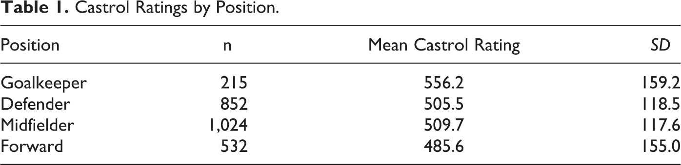
The differences between positions are significant on a one-way analysis of variance (F = 15.2, df = 3, p < .001) and create an unwanted complication. Consider two “average” teams, each consisting of an average goalkeeper, with average defenders, average midfielders, and average forwards, but with different numbers of outfield players in each position; because of the differences in mean ratings by position, the abilities of the two teams as measured by the sum of their Castrol ratings would differ from one another. To overcome this problem, the ratings were standardized within position. First, each player’s rating was converted to a z-score within position. For convenience, the ratings were then transformed back to their original scale; the z-scores were multiplied by the grand SD (over the entire data sample) and the result added to the grand mean (of the entire data sample). In this way, the mean ratings for each position and the SD of ratings within each position were made equal to each other (and to the mean and SD of the entire data sample). Using standardized ratings ensures that a team of average players has the same total rating irrespective of the distribution of players among positions, and standardized ratings are used throughout this article.
Total team ability (A)
A football match lasts for 90 min. Clearly, an individual who is on the field for less than 90 min has less impact on the team’s total ability than one who plays the full match. Total team ability for a match is therefore calculated as the sum of the participating player abilities weighted by the proportion of minutes played:
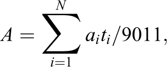
where A is the total ability of the team, N is the number of players in the team, and ai and ti are the ability and minutes played by player i, respectively. The divisor 11 is simply a scaling constant to bring A onto the same scale as a single player.
Heterogeneity (H)
Team heterogeneity is measured by the Gini coefficient, first described by Gini (1912, 1921). The Gini coefficient is an index of inequality frequently used in economics and ecology and summarizes the dispersion of some quantity of interest among the members of a population. In this case, the quantity of interest is Castrol rating points, and the population is the players in the team. The coefficient ranges between 0 and 1. A Gini coefficient of 0 expresses maximum homogeneity, where the quantity of interest is allocated equally throughout the population; a Gini coefficient of 1 expresses maximum heterogeneity, where all the quantity of interest is allocated to a single member of the population and none to the remaining members. For a modern treatment of the Gini coefficient, see, for example, Milanovic (1997) or Yitzhaki (1998).
Computing the heterogeneity of a football team is not however straightforward, because the composition of a team typically changes during a match. One type of change is the substitution of one player by another; substitutions are common and are made either because a player sustains an injury or, more usually, for tactical reasons. One or more substitutions were made in over 99% of the team performances in the data set. Furthermore, a player may be sent off the field by the match referee for a serious infringement of the rules, an event known as getting a red card or being red-carded. A player shown a red card is not replaced, leaving his team to complete the match with fewer than the Regulation 11 players. This is a moderately common occurrence, and one or more red cards were issued to a team on about 12% of occasions.
To account for the changes in personnel and therefore in team heterogeneity during the match, the players on the field were identified at the start of the match and at 10-min intervals thereafter. The Gini coefficient of the players’ Castrol ratings was calculated at each time point, and the average coefficient for the 10 time points was taken as the heterogeneity of the team for that match.
Red cards (R)
This is a binary variable, scored as 1 if a team was shown one or more red cards during the match and 0 otherwise.
Goals scored (G)
Goals scored during the match is the measure of team performance and the dependent variable in the analysis.
Modeling Strategy
The dependent variable for the analysis is goals scored. In this data set, goals scored is distributed as a slightly under dispersed Poisson distribution (mean = 1.38, SD = 1.24), with the difference from a Poisson distribution being nonsignificant on a one-sample Kolmogorov–Smirnov test (KS statistic = 1.24, p = .093). The distribution of goals scored suggests the use of the generalized linear model, which allows dependent variables that are not normally distributed to be modeled by choosing an appropriate link function. In the present case, we use a logarithmic link function which is appropriate for Poisson data.
A further consideration is the structured composition of the data set which is a potential source of nonindependence between observations. Violations of the assumption of independence may potentially bias standard errors and result in incorrect statistical inferences, so from a data modeling perspective it is important to assess the degree of nonindependence and incorporate it in the data model if necessary.
There are two sources of nonindependence in the data. First, each team provides multiple observations, which could potentially be more similar than observations selected at random. Second, a football match involves two teams, and the teams that make up the match dyad interact and mutually influence one another, so that the individual outcomes for each depend on the attributes and actions of both. In the language of dyadic analysis (Kenny, Kashy, & Cook, 2006, p. 145), an actor effect occurs when a dyad member’s outcome is influenced by its own attributes or actions, and a partner effect occurs when a dyad member’s outcome is influenced by the attributes or actions of the other member. In a football match, for example, the number of goals scored by a team depends not only on its own strength (an actor attribute) but on the opposition’s strength (a partner attribute) as well. In our data set, three matches were played at a neutral venue, so in the vast majority of cases, one member of the match dyad was the home team and the other was the away team. The ability to differentiate between dyad members in this way means the dyads are distinguishable. This is important because the analytical treatment of distinguishable dyads differs somewhat from the treatment of and nondistinguishable dyads. To preserve the characteristic of distinguishability, the matches played at a neutral venue were eliminated from the analysis.
To account for potential nonindependence in the data, a mixed effects model was adopted.
Analysis and Results
Univariate Statistics and Correlations
Table 2 shows the univariate statistics for the study variables and their intercorrelations. Note that each match is represented by two records in the data set, one for the home team and one for the away team; in one record team, i is the home team and team j is the away team, with the roles being reversed in the second record. Because of this double-entry or pairwise structure (Kenny et al., 2006, p. 18), pairs of corresponding actor partner variables (i.e., actor total ability ↔ partner total ability; actor heterogeneity ↔ partner heterogeneity; actor red cards ↔ partner red cards; goals for ↔ goals against) appear twice in the data set, once in the order i, j and once in the order j, i. Significance levels for the correlations between these variables are therefore based on the number of matches (1,822) rather than the number of observations, otherwise the same data would be counted twice. The affected correlations are superscripted in Table 2.
Univariate Statistics and Intercorrelations for Study Variables.
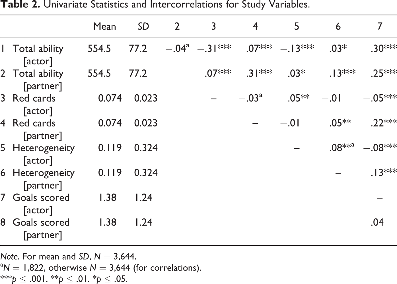
Note. For mean and SD, N = 3,644.
aN = 1,822, otherwise N = 3,644 (for correlations).
***p ≤ .001. **p ≤ .01. *p ≤ .05.
A Dyadic Model for Team Composition and Performance
The team composition model described next examines the influence of actor and partner composition variables on team performance. The dependent variable is the number of goals scored (G), which is assumed to follow a Poisson distribution, and log expected values are modeled as a linear combination of independent variables using a logarithmic link function.
Before discussing the model, it is important to note an unfortunate issue of terminology. The terms “random” and “fixed” effects as used in the mixed model literature overlap confusingly with the terms as commonly understood by economists (and others). Indeed, Gelman (2005) has pointed out that the distinction between fixed and random effects has been defined in at least five different ways, some of which are contradictory.
In the economic literature, the distinction between fixed and random effects is that “…‘fixed’ effects variables are correlated with the other included regressors while ‘random’ effects are not.” (D. C. Coates, personal communication, January 6, 2016). In the mixed model literature, fixed effects are constant across individuals, but random effects vary. For example, the mixed model yij = aj + βxij (e.g., for pupil i in school j) has a constant (fixed) slope for pupils and different (random) intercepts for schools, while the model yij = aj + β j xij has different (random) slopes and intercepts. To avoid confusion, Gelman suggests classifying the coefficients in a mixed model as constant if they are the same for all groups and varying if they differ across groups. That recommendation is followed here.
The first step of the modeling procedure examined the varying effects. Two baseline models were estimated; the first model (R1) contained an intercept term and a varying intercept for team nested within league, and the second model (R2) additionally contained a varying intercept for match. The results are shown in the first two columns of Table 3.
Team Composition Models for Performance.
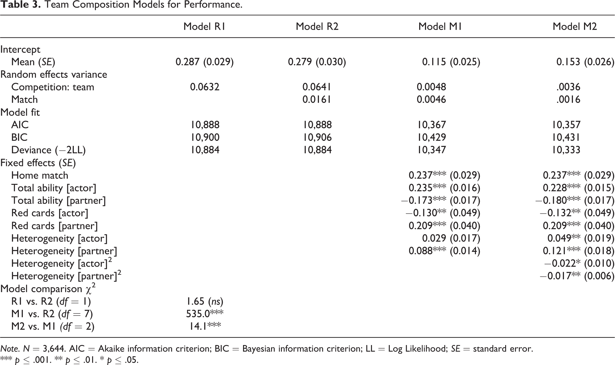
Note. N = 3,644. AIC = Akaike information criterion; BIC = Bayesian information criterion; LL = Log Likelihood; SE = standard error.
*** p ≤ .001. ** p ≤ .01. * p ≤ .05.
The Akaike information criterion (AIC) and deviance measures for R1 and R2 are almost the same, and the model comparison χ2 is nonsignificant, indicating that allowing the intercept for match to vary does not improve the model significantly; indeed, the lower Bayesian information criterion (BIC) for model R1 suggests the simpler model might be the preferable formulation. However, because of the theoretical importance of the dyadic data structure to our arguments, it was decided to retain the varying match intercept in the subsequent analysis and treat R2 as the baseline model for subsequent model comparisons.
The next step in the modeling procedure was to add the constant effect regressors. The regressors were the dyad member indicator (venue, coded as 1 = home, 0 = away) and the total team ability, heterogeneity, and red card indicators of both teams in the match dyad. Red card indicators were included in the model because they affect the composition of the teams by eliminating players. The constant portion of the model is described in the following equation, where Gi is the number of goals scored by team i in match k, with match subscripts being omitted throughout for clarity:

where i and j are the two teams in the match dyad, and the independent variables denoted by A, H, R, and V are defined in the measures section above. The βs have the usual meaning, with the expanded subscripts a and p being used to denote the “actor” and “partner” members of the dyad (i.e., team i and the opposition), respectively.
The estimates for this model are reported under model M1 in Table 3. Two variations to M1 were also examined. Following the suggestion of Kenny, Kashy, and Cook (2006, p. 174), the first variant included interactions between the dyad member indicator and the other regressors. However, none of the interactions were significant, and this model is not reported. The second variant added quadratic terms for actor and partner heterogeneity and was examined because Papps et al. (2011) found significant quadratic effects. Estimates for this model are reported under model M2 in Table 3.
Note that to simplify interpretation of the model coefficients, all the independent variables were standardized to have a mean of 0 and SD of 1. For the purposes of interpreting the constant effects, note also that the goals scored by team i is the same as the goals conceded by team j. This means that the partner coefficients for goals scored can also be interpreted as actor coefficients for goals conceded. For example, the effect of team js ability on goals scored by team i is a partner effect which is gauged by β 1p , but this term can also be viewed the actor effect of team js ability on goals conceded by team j.
The three fit measures for model M1 are substantially lower than those for R2, demonstrating that adding the constant effects produces a substantial improvement in fit. This improvement is also reflected in the reductions in the variance of the varying effects for team and match. Furthermore, the model comparison test (χ2 = 535.0, df = 7, p < .001) confirms that the improvement in model fit is highly significant.
Turning to the evaluation of the quadratic model M2, the smaller values of AIC and deviance for this model indicate that adding quadratic heterogeneity terms results in a better fit, and the model comparison test (χ2 = 14.0, df = 2, p < .01) indicates the improvement is significant; however, the BIC measure of fit is similar for both models, indicating that neither model is clearly preferable to the other. At the expense of some additional complexity, the analysis in the following section is based on model M2; however, using M1 instead produces very similar conclusions.
The regression intercept of .153 implies that the average team competing away from home (against an average team) scores 1.2 goals. The significant positive coefficient for home match implies that teams score more goals playing at home than away; this is a well-established feature of football (and other sports) known as home advantage. The coefficient for home match implies the average team scores a further 27% (i.e., 0.40) goals at home, a result in line with other studies; for example, Boyko, Boyko, and Boyko (2007) found a home advantage of 0.4 goals per match in the English Premier League between 1992 and 2006.
The positive coefficient for actor team ability shows that teams with higher ability score more goals, while the corresponding negative partner coefficient shows that teams score fewer goals against high ability teams (i.e., higher ability teams concede fewer goals). These findings imply that the task of scoring goals and the task of defending against them both contain an additive component. If we define a good team as one with a total ability 1 SD (77 points) above the mean, the actor coefficient implies that a good team will score 26% more goals than an average team, while the partner coefficient implies that a good team will concede 16% fewer goals than an average team. Ability seems to have asymmetrical effects on goals scored and conceded, and a Wald test was conducted to determine the significance of the asymmetry. The null hypothesis that the actor and partner coefficients for ability were equal in magnitude and opposite in sign was rejected (χ2 = 4.5, df = 1, p < .05), implying that the asymmetry is significant and that total ability has a somewhat larger effect on goals scored than on goals conceded.
As expected, the actor coefficient for red cards is negative, and the partner coefficient is positive, indicating that red-carded teams score fewer goals and concede more. Although the effect on goals conceded (an increase of 23%) is almost twice as large as the effect on goals scored (a reduction of 12%), a Wald test does not reject the hypothesis of equal and opposite coefficients (χ2 = 1.6, df = 1, p > .05). This means we cannot conclude the asymmetry in red card effects is statistically significant.
The goals a team scores depends on both its own heterogeneity and the heterogeneity of the opposition. Examination of the first-order and quadratic coefficients for actor heterogeneity shows that increasing heterogeneity is associated with increases in goals scored up to 1.1 SDs above the mean, after which further increases in heterogeneity begin to produce a decline in goals scored. For partner heterogeneity, the linear term is larger and the quadratic term is smaller, increases in partner heterogeneity are associated with increases in goals scored over most of the range, and the direction of the association only reverses when heterogeneity is more than 3.5 SDs above the mean. A Wald test showed that the first-order coefficients for actor and partner heterogeneity are significantly different (χ2 = 7.7, df = 1, p < .01); in addition, a test for the total effects of the first-order and quadratic coefficients was significant (χ2 = 11.0, df = 1, p < .001), confirming that actor and partner heterogeneity effects are significantly different. To summarize, increasing actor heterogeneity increases goals scored, while increasing partner heterogeneity increases goals scored even more. The overall effects of heterogeneity on performance can best be understood from Figure 1. Here, we imagine two teams of average total ability with Team 1 playing at home and Team 2 playing away. Team 2 has constant average heterogeneity and we examine the impact on the match score as the heterogeneity of Team 1 increase from 2 SDs below the mean to 2 SDs above the mean.
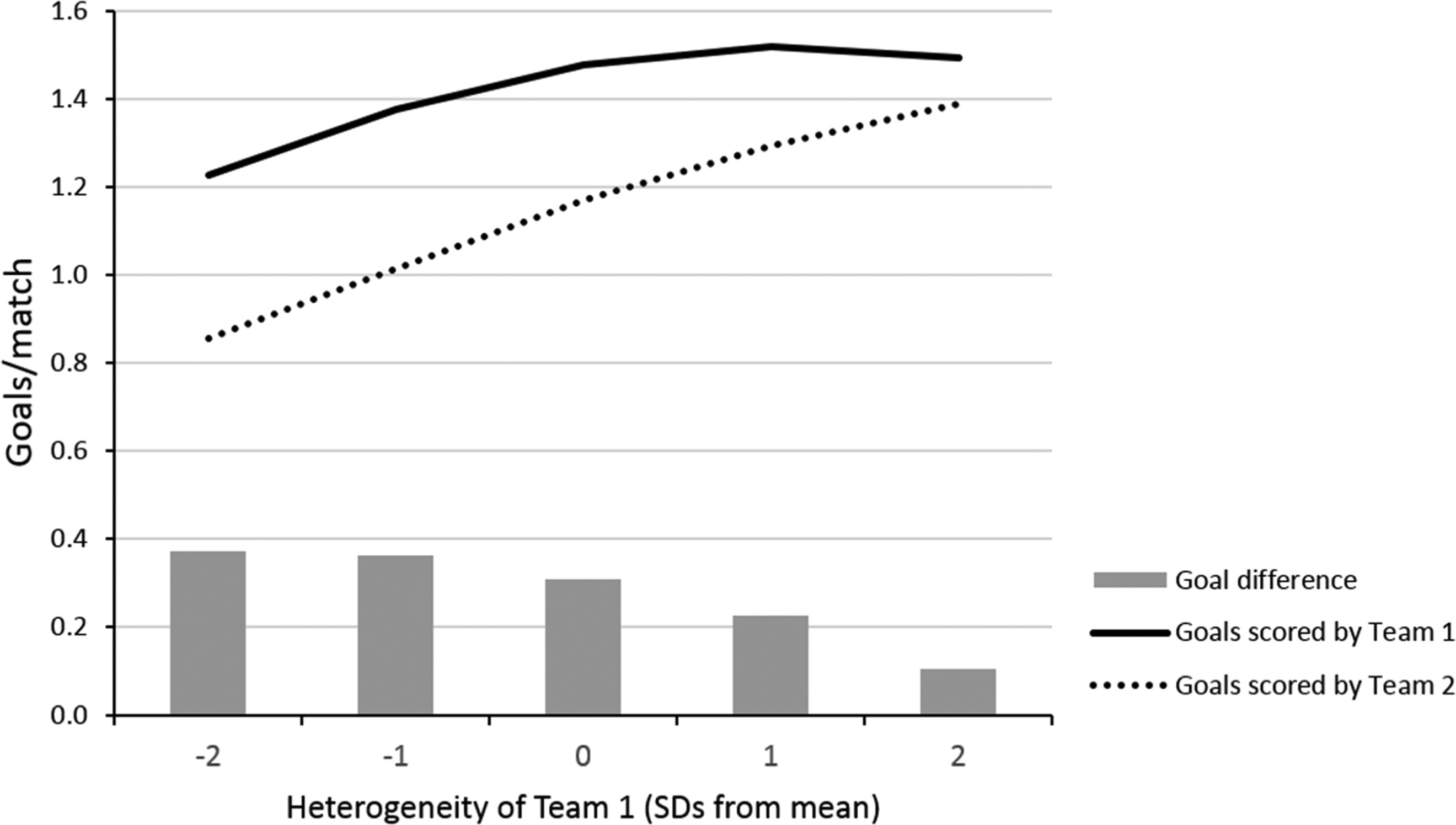
Effects of heterogeneity on goals per match scored and conceded by Team 1.
Inspection of Figure 1 shows that as its heterogeneity increases, Team 1 scores more goals; but Team 2 scores even more, as from its point of view, the heterogeneity of its partner is increasing. Put another way, as the heterogeneity of Team 1 increases, it scores more goals but concedes even more. The net effect on Team 1 is that as its heterogeneity increases, its goal difference, which represents superiority over the opposition, is reduced. Overall therefore, Team 1’s performance decreases as its heterogeneity increases.
Discussion
The unique contribution of this article is that the effects of team composition on attack and defense are estimated separately, giving further insights into the relationship between team composition and football performance.
The findings indicate a strong element of task additivity in both attacking and defending, and as would be expected, high ability teams outscore low ability teams and concede fewer goals. There is weakly significant evidence that partner ability has a stronger relationship to scoring than to conceding. This could simply be a property of the ability measure used; however, if that were the only reason for the difference, we would expect that partner heterogeneity would also be more strongly related to scoring than conceding (to see this imagine a zero correlation between ability and conceding); but in fact the reverse holds true.
Overall, heterogeneous football teams are found to perform less effectively than their more homogeneous counterparts, confirming findings previously reported by Franck and Nüesch (2010). There are substantial differences between the two studies. For example, Franck and Nüesch’s data set covered multiple seasons for a single league, the dependent variable was goal difference, the model equation was nondyadic, heterogeneity was operationalized by the coefficient of variation, and talent was operationalized using both objective and subjective measures. Despite these differences, the conclusions of the two studies are broadly comparable. Franck and Nüesch found that a 1 SD increase in heterogeneity is associated with a reduction of 0.14 in goal difference per match; in this study, the relationship is nonlinear, but the average is approximately 0.07 goals per SD. We can conclude that the reduced performance of heterogeneous teams in elite football is robust across data sets and measurement methods.
Because pay and performance in sports teams are positively related (e.g., Nüesch, 2009; Frick, 2011), this aspect of the findings is aligned with previous studies on pay structures in sports teams which have also found increased heterogeneity to be associated with reduced team performance (Coates et al., 2016; Depken, 2000; Frick, Prinz, & Winkelmann, 2003). Such performance decrements have been attributed to a loss of group cohesion caused by perceived pay inequities. However, this mechanism cannot explain why attacking performance should be elevated in heterogeneous teams, a finding that suggests cohesion theory cannot be the sole explanatory mechanism underlying performance.
The results of this study suggest that attack and defense respond differentially to team composition because they are different tasks having distinct dynamics. The effect of heterogeneity on scoring goals is beneficial, indicating that this task is on balance disjunctive. This would be a plausible conclusion. Attacking benefits from heterogeneity because attacks on goal are substitutable or at least contain a substitutable component. Of course, players usually need to collaborate to mount an effective attack, but where one strategy or one attacker fails to breach the opposition defense, another may succeed. As Prat (2002) demonstrated, such dynamics favor heterogeneous groups.
Conversely, heterogeneity has a detrimental effect on defending and heterogeneous teams tend to leak goals. This is evidence that defending is a conjunctive task. Although defenders can cover for one another to some extent, a weak link in the defense is a constant vulnerability which can be exploited by the opposition, leading to depressed defensive performance. An interesting question is whether the task dynamics found in this study are unique to football or whether they are also characteristic of other invasion sports such as American football, rugby, and basketball. Is attacking inevitably disjunctive and is defending inevitably conjunctive? A common conceptual model for understanding the dynamics of attack and defense in multiple sports would be of substantial theoretical interest in sports science.
Finally, as pay disparities and differences in ability generally go together, further research is warranted on the joint role of both types of diversity on team performance. Is the effect of pay disparity mediated through its connection to ability or do both team cohesion and task-related processes influence team performance?
Footnotes
Declaration of Conflicting Interests
The author(s) declared no potential conflicts of interest with respect to the research, authorship, and/or publication of this article.
Funding
The author(s) received no financial support for the research, authorship, and/or publication of this article.