
Abstract
The disparity between athlete compensation and major sports revenues has produced criticisms of The National Collegiate Athletic Association (NCAA)’s Collegiate Model of athletic competition. In defense, the NCAA argues that it promotes competitive balance. One implication is that moving toward a professional model would reduce balance. The present article tests this hypothesis by comparing competitive balance in Power-5 conference football to that for the professional National Football League (NFL) using a variety of balance metrics. The results provide no support for the NCAA’s implicit hypothesis of less balance in the NFL, undermining competitive balance as a legitimate defense of the NCAA’s Collegiate Model.
Introduction
The National Collegiate Athletic Association (NCAA), the primary governing body of American college sports, follows what it describes as the Collegiate Model of athletic competition. The model’s two key components are the athlete-as-student and amateurism, the latter referring to compensation limited to the traditional athletic scholarship. The athlete-as-student component is not controversial. But the NCAA has been under attack in recent years because of the amateurism component and the associated restrictions on athlete compensation. The focus of critics is the big money sports of football and men’s basketball, where many schools earn revenues exceeding US$100 million and therefore could significantly increase compensation. A major defense of its Collegiate Model proffered by the NCAA is that it promotes competitive balance. The implication is that a movement toward a professional model of some kind (e.g., higher pay) would reduce balance. Given the absence of a counterfactual, a direct test of this hypothesis is impossible.
The purpose of this article is to conduct an alternative test of the NCAA’s implied hypothesis by comparing competitive balance among top tier college football schools with that of a professional model as manifest by the National Football League (NFL), America’s premier professional league. The statistical analysis covers the 20-year period 1998-2017. It is based on the final regular season records of the current 32 NFL teams and 62 of the current members of the so-called Power-5 collegiate football conferences (leagues), the top echelon of college football. 1 We treat the Power-5 schools as a “closed” league, like the NFL, by excluding from their records all games against non-Power-5 opponents. Standard competitive balance metrics are used, drawn from the sports economics literature. The results refute the NCAA’s implicit hypothesis of less balance in the NFL, undermining the competitive balance defense of the Collegiate Model.
Related Work
A few prior studies report balance comparisons between collegiate football and the NFL with mixed results, although the comparisons are an incidental part of their analyses. Each of these includes the Power-5 conferences, like the present article. However, unlike the present article, they generally include most or all schools in non-Power-5 Football Bowl Subdivision (FBS) conferences and all games against non-Power-5 opponents.
Berri (2004) computes competitive balance metrics for the NFL for 1987-2000 and 11 NCAA Division I-A (FBS) football conferences for 1995-2001, including the Power-5. His single metric is the same normalized annual league standard deviation of team winning percentages used below (ratio of standard deviations [RSD], see Equation 6). He reports an RSD value of 1.46 for the NFL and a mean of 1.55 for the 11 college conferences, indicating better annual balance in the NFL (Berri, 2004; Tables 1 and 2).
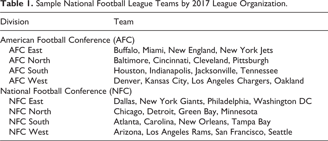
Sample National Football League Teams by 2017 League Organization.
Sample Power-5 Schools by 2017 Conference Membership.
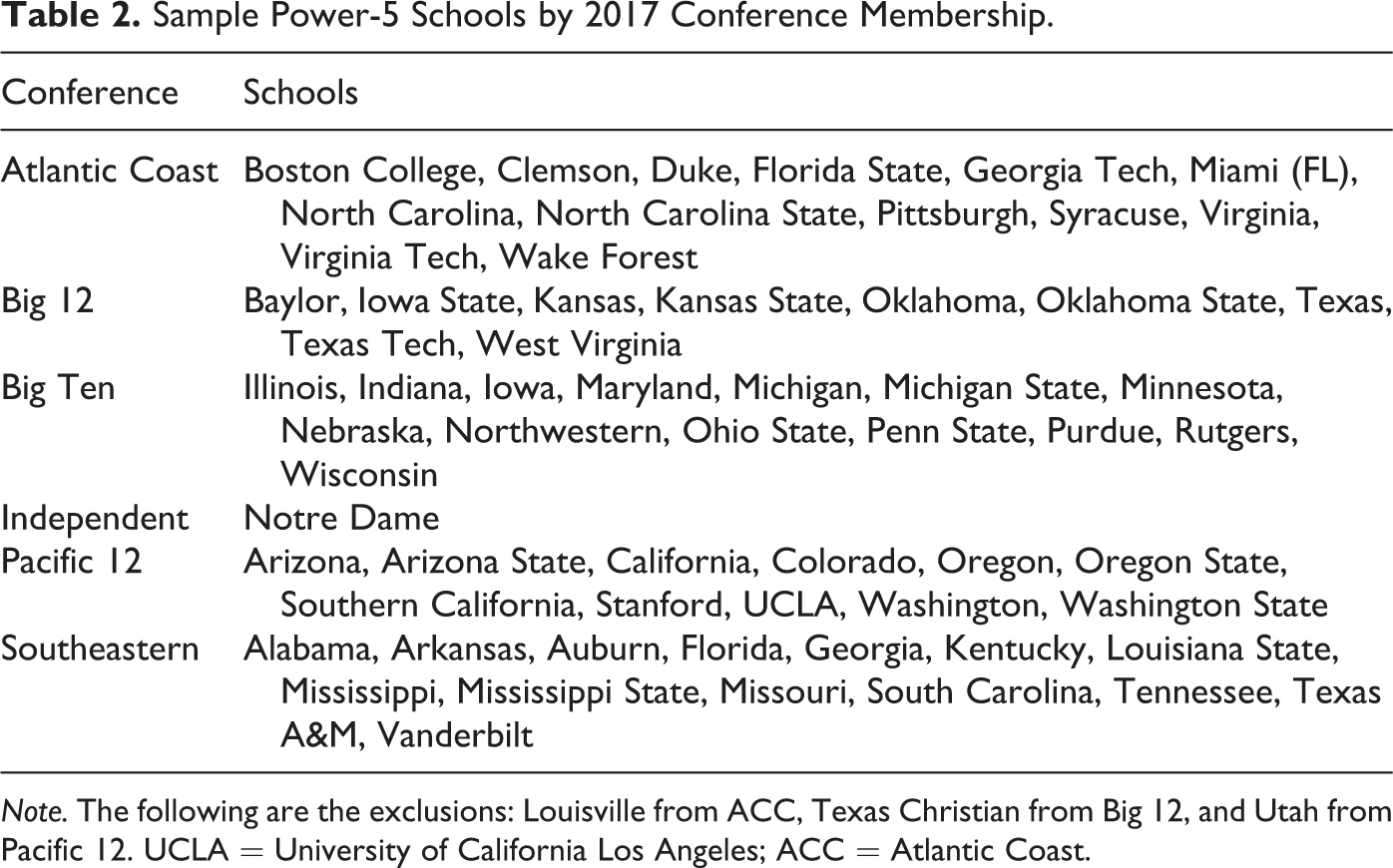
Note. The following are the exclusions: Louisville from ACC, Texas Christian from Big 12, and Utah from Pacific 12. UCLA = University of California Los Angeles; ACC = Atlantic Coast.
Baird (2004) examines the distribution of cumulative football team winning percentages for schools in 10 Division I-A (FBS) conferences for 1985-2001, also using a single metric. She finds that 22% of these schools are within 1 standard deviation of .500. She compares this to professional football data reported in Quirk and Fort (1992) where “only 13.3% of teams are this close to .500” (Baird, 2004, p. 230), indicating less balance in professional football.
More recently, Mills and Winfree (2017) compare competitive balance between all FBS schools and the NFL for the period 1990-2016. One of their two metrics corresponds to our normalized standard deviation RSD (see Equation 6). The second metric is the correlation between successive season winning percentages computed annually, a measure of year-to-year churning in league standings. The analysis consists of visual observations of time series graphs, without summary statistics. The authors’ RSD analysis suggests that “there tends to be equal or less concentrated distribution of wins across NCAA football,” that is, equal or more balance among FBS schools. However, their correlation measure indicates “substantially more turnover” (better balance) in the NFL.
Salaga and Fort (2017) report mean competitive balance measures by decade since league formation for the Power-5 conferences and the NFL. They use the same two metrics as Mills and Winfree (2017) and obtain similar qualitative results. Salaga and Fort (2017) report decade averages but do not conduct statistical tests. They observe that “from the 1960s onward the college conference [RSD] values are comparable to those…of the National Football League” (p. 31). For their successive season winning percentage correlation metric, they find that “the professional version of football shows much less correlation [more balance] than the college version” (p. 33).
Competitive Balance and the NCAA’s Collegiate Model
As noted above, the NCAA’s Collegiate Model of athletic competition has two key components: the athlete-as-student and amateurism. The objective is “maintaining a line of demarcation between student–athletes who participate in the Collegiate Model and athletes competing in the professional model,” that is, between college sports and professional sports. 2 Certainly in the case of football, the NFL qualifies as an appropriate counterpoint.
Although asserting that its model promotes competitive balance (see below), the NCAA provides no general explanation for the linkage. The NCAA Division I Manual (2016), a 395-page compendium of its rules and regulations, neither asserts nor explains a connection between competitive balance and the Collegiate Model or either of its components. Surprisingly, the Manual mentions the term “competitive balance” only once, stating that athletic department staff should be managed “in a manner consistent with the need for competitive balance” (NCAA, 2016, p. 27).
The Manual also uses the term “competitive equity,” but its meaning is unclear. The Manual begins with a statement of 16 Principles for Conduct of Intercollegiate Athletics. The 10th is The Principle of Competitive Equity (NCAA, 2016, p. 4): The structure and programs of the Association and the activities of its members shall promote opportunity for equity in competition to assure that individual student-athletes and institutions will not be prevented unfairly from achieving the benefits inherent in participation in intercollegiate athletics.
As with the Manual, neither of the NCAA’s two websites, NCAA.org and NCAA.com, contain a general discussion of the causal connection between the Collegiate Model and competitive balance. However, in discussing its defense against a recent antitrust lawsuit, the NCAA makes the claim on NCAA.org that the Model promotes competitive balance, linking it to the amateurism component.
As noted above, the main criticisms of the Collegiate Model focus on the lucrative sports of football and men’s basketball. The on-field performance of the athletes is, of course, the main attraction for fans and the source of the associated money, but athlete compensation is restricted to the traditional scholarship. This is comprised mainly of free tuition, room and board, books, and the recently adopted “cost of attendance” stipends limited to a few thousand dollars annually. There is general agreement that the value of these scholarships is much less than the revenue generated by top athletes in major football and basketball programs. 3 The resulting rents are captured by the universities that sponsor these programs and by the NCAA. The critics argue that a significant portion of these rents should be shared with the athletes. This, of course, is at odds with the amateurism component of the Collegiate Model.
The recent O’Bannon v. NCAA antitrust case was an attempt at achieving one form of athlete pay increase. Plaintiffs argued that athletes should be able to receive monetary payments for the use of their “name, image, and likeness” (NIL), contrary to NCAA rules promoting amateurism. 4 As one main element of its defense, the NCAA stated: “The Collegiate Model maintains a competitive balance among schools and across conferences.” 5 A key defense witness in the case argued that NIL payments “…would ultimately result in a destruction of competitive balance among the paying schools.” 6 Also, in an O’Bannon Post-Trial Brief, the NCAA stated that “The challenged rules [against NIL payments] promote competitive balance” (Defendant NCAA’s Post-Trial Brief, p. 25). To our knowledge, the NCAA has never presented statistical evidence in support of these claims.
By contrast, economists have long viewed the NCAA as a monopsony cartel of sports-sponsoring colleges and universities, that is, a monopsony buyer of athletic talent. Several studies have analyzed the effect of its regulations, including pay restrictions, on competitive balance. The weight of the evidence suggests that the NCAA’s economic regulations most likely reduce balance. 7 Except for the papers summarized above, this research does not involve collegiate–professional balance comparisons.
Sample Description
The sample period is arbitrarily selected as 20 years from 1998 to 2017, a period long enough to measure intertemporal competitive balance, that is, changes in the relative performance of teams over time. All current 32 NFL teams are included, listed in Table 1, with 30 having operated continuously over the 20-year period. The exceptions are the Cleveland Browns with 19 years of NFL competition (1999-2017) and the Houston Texans with 16 years (2002-2017). 8 The NFL is a closed league, that is, members play games only with other members. Its regular season (excluding playoffs) consisted of 16 games for every team in each year throughout 1998-2017.
In contrast, the NCAA includes over 1,000 colleges and universities, organized by various levels of competition. The highest level is the FBS, with 10 conferences plus a few independent schools. Within this group, five conferences, known as the Power-5, have dominated. These are the Atlantic Coast (ACC), Big 12, Big Ten, Pacific 12, and the Southeastern, all of which have operated continuously since 1998 (and earlier). For example, current Power-5 schools including major football independent Notre Dame have occupied 190 of the 200 Associated Press poll final top 10 slots (95%) during 1998-2017. And in 2017, current Power-5 schools including Notre Dame had a record of 87 wins and only 15 losses against non-Power-5 FBS schools, a .853 winning percentage. The record against non-FBS schools was 39-1, a .975 winning percentage. In 2014, the special status of Power-5 conferences was recognized with a grant of significant autonomy in terms of governance and rule-making within the NCAA’s overarching regulatory structure.
Accordingly, the collegiate sample of 62 teams includes 61 of the 64 current members of the Power-5 conferences, plus Notre Dame (see Table 2). Three current Power-5 conference members are excluded because they were major conference members for 12 or fewer years during 1998-2017. 9 We do not conduct separate conference-by-conference comparisons because significant changes in conference alignments occurred during the study period. Several schools moved from one Power-5 conference to another, and others moved into or out of the Power-5 group. A sixth major conference, the Big East, ceased operation after the 2012 season. It had operated since 1998 (and earlier) and was considered equivalent to the Power-5 conferences. Most of its members switched to the ACC, Big Ten, or Big 12 between 2004 and 2013 and are included in the sample. 10
The Power-5 schools, unlike the NFL, do not operate as a closed league. During 1998-2017, they typically played a regular season schedule of 11 or 12 games, with 7–9 of these against opponents in their own conference. Of the remaining nonconference games, roughly half were against other Power-5 schools and the remainder against non-Power-5 schools. In the present analysis, however, we treat the Power-5 schools as a closed league. We ignore conference affiliations, combining for each school all games against other Power-5 opponents, including Big East members from 1998 to 2012, into a single win–loss record and associated winning percentage. 11 Games against opponents other than members of Power-5 conferences and the Big East are excluded from each school’s win–loss record. This avoids an artificial reduction of winning percentage standard deviations because of the Power-5 dominance over other schools (see above). Thus, as defined, the sample of 61 Power-5 schools plus Notre Dame constitutes a closed “league” comparable to the 32 NFL teams. 12
Only regular season games are included in the win–loss records for both the Power-5 and NFL samples. 13 Postseason games in both leagues are between teams in the upper end of their respective win distributions. Since the overall winning percentage for all teams in the postseason must be .500, combining the postseason and regular season records would on average reduce the winning percentage of leading teams. Thus, competitive balance metrics would be artificially reduced. This is likely to affect the Power-5 more than the NFL, as a larger percentage of Power-5 teams are involved in postseason games, and these games generally are a larger proportion of the fewer regular season games played by college teams.
Measuring Competitive Balance
Competitive balance or parity among teams in a sports league means that member teams are evenly matched. Thus, individual game outcomes and season-long championship competitions are more uncertain, and thus more exciting for both athletes and fans. The resulting increase in interest among fans, of course, promotes the league’s long-run financial viability. This presumably is why the NCAA regards competitive balance as “good.” For example, in defending the O’Bannon case, the NCAA (2014) stated that “Upsetting the current level of competitive balance would negatively affect the popularity of college sports” (p. 26).
Balance implies less dispersion among teams in seasonal league standings. It also means that over a period of several years, many different teams will contend for league and national championships. Competitive balance metrics seek to quantify these concepts using data on team win–loss records and positions in league standings. Evans (2014) presents an exhaustive and detailed survey of the statistical measures of competitive balance in sports, including all metrics used below.
Multiple metrics are used in the present analysis because the theory does not suggest a “best” one, and the various metrics capture different aspects of balance (Fort & Maxcy, 2003). Also, a consistent pattern across several metrics indicates robust results.
Variance and standard deviation metrics
One group of competitive balance metrics focuses on the variability of team winning percentages, within seasons and over time. In each league, a distribution of winning percentages exists that includes all teams in every year of the 20-year study period, with an overall variance VAR that can be partitioned as follows: 14

VARcum, the “cumulative variance,” is the variance of cumulative winning percentages across league members. VARtime, the “time variance,” is the mean of individual teams’ annual winning percentage variances about their own means over the study period:

where VART is the variance of each team’s winning percentage variance over the period and T is the number of teams.
For a given total variance VAR, a lower (higher) cumulative variance and higher (lower) time variance indicate that competitive balance is higher (lower). If VAR changes, the interpretation is more complex. However, it remains true that the greater the proportion of VAR accounted for by the time variance, the greater the competitive balance. This metric can be defined as the percentage of the total variance accounted for by the time variance:

As %Time increases, the time variance is a larger proportion of the total, and the cumulative variance is a smaller proportion, indicating greater competitive balance over the period. 15
In addition to the %Time statistic, we use three other related variability metrics. The first is the annual within-season standard deviation of winning percentages of league members. Greater competitive balance implies less variation in wins among teams, winning percentages closer to .500, and a lower standard deviation in any given season. While this probably is the most commonly used balance measure, it excludes the important time series dimension. This is captured by the second metric: the mean of the time series standard deviations for league teams, where each team’s standard deviation is the square root of VART in Equation 2. More year-to-year variability in winning percentage for each team indicates more churning in league standings and greater competitive balance over time. The third metric is the standard deviation of cumulative winning percentages among teams for the sample period, the square root of VARcum in Equation 1. Greater balance means that high winning percentages in one year are offset by low ones in another year, causing cumulative winning percentages to be close to .500. The result would be less variation among teams in their cumulative winning percentages, that is, a lower standard deviation.
Concentration metrics
A second group of competitive balance metrics examines the extent to which strong performance is concentrated among a few league teams over the 20-year study period. Strong performance is indicated by a leading position in the final regular season league standings. Greater balance implies less concentration, with strong performances more widely dispersed among teams. We examine the concentration of league champions and the concentration of teams in the top N positions in the rank-ordered standings.
A standard concentration measure is the Herfindahl–Hirschman Index (HHI), calculated as follows:

where Si is the ith team’s share of championships or appearances in the top N positions; and the summation is over all teams in the league. Shares are measured as percentages; thus, HHI can vary from (near) 0 to 10,000.
The second concentration metric is the percentage of all league teams that won championships or made at least one appearance in the top N positions during the 20-year study period. A lower percentage indicates greater concentration and less balance.
Normalization for league size and games played
Comparisons between the Power-5 and the NFL can be affected by differences in the number of teams and the number of games played per team that can create statistical biases in the balance measures (Evans, 2014). The Power-5 has 62 teams and the NFL has 32. Other things being equal, leagues with more teams tend to produce balance measures that indicate greater annual balance, for example, lower standard deviations or less concentration. This produces a bias against the NFL with its fewer teams. The second obscuring difference is the number of games constituting a season, 16 for the NFL and an average of about 9.3 for the Power-5. Other things being equal, leagues that play more games tend to produce balance measures that indicate greater balance. This produces a bias against the Power-5 with its fewer games.
The standard deviation competitive balance metrics can be normalized for the number of games played by comparing them to an “ideal” standard deviation associated with “perfect” competitive balance. 16 The usual definition in the literature is that in every game, both teams have an equal chance of winning. The result is a binomial distribution of team wins with a probability of “success” (winning) equal to .5 in all games, yielding a nonzero standard deviation for the winning percentage. This is referred to as the idealized standard deviation (ISD), calculated as follows (Quirk & Fort, 1992, p. 245):

where G is the number of games played by each team. The normalized standard deviation is commonly called the ratio of standard deviations (RSD), defined as:

where ASD is the actual standard deviation of winning percentages. This normalization allows comparisons between standard deviation balance measures of leagues that play differing numbers of games.
The number of games played by each team in the NFL is constant at 16 throughout our study period, yielding a constant annual ISD of .125. For the Power-5 schools, however, the number is not constant. For individual teams, the number of games played against other Power-5 schools annually varies from 7 to 12. Accordingly, we compute annual RSDs from annual ISDs based on the mean number games played by sample schools in each year, which varies from 8.98 to 9.66. Thus, the annual Power-5 ISD varies from .161 to .167.
The HHI also can be impacted by differences in the number of league members and/or games played, which influence the maximum and/or minimum possible values and therefore the range of possible values. Normalized HHIs (N-HHIs) account for these differences (Evans, 2014; Owen, Ryan, & Weatherspoon, 2007). Let HHI represent the actual value, and HHIMAX and HHIMIN represent the maximum and minimum possible values. For the top N league positions, HHIMAX occurs if the same N teams occupy those positions every year. HHIMIN occurs if the 20 × N total top positions during our study period are evenly distributed among all league teams. The normalized value N-HHI is then calculated as follows:

This is the amount by which HHI exceeds its minimum possible value, expressed as a percentage of its possible range. The N-HHI can vary between 0% and 100%, with greater values indicating more concentration and less competitive balance.
The concentration measures related to the top N positions must be normalized to account for the different number of teams in the two leagues. This avoids bias against the Power-5 with its larger number of teams. In particular, the top N positions should include the same proportion of total members for each league. In other words, the top Nth position in each league should correspond to approximately the same percentile of rank-ordered teams. We arbitrarily select the top 10 (N = 10) and top 20 (N = 20) for the Power-5. Since the NFL has 32 teams, about half the Power-5’s 62, this implies a comparison with the top 5 (N = 5) and top 10 (N = 10) for the NFL. The Power-5’s Top 10 and the NFL’s Top 5 are each at about the 16th percentile. Similarly, the Power-5’s Top 20 and the NFL’s Top 10 are at about the 32nd and 31st percentiles, respectively. The same issue arises when examining the concentration of league champions, that is, the “top 1” position. To adjust for the differing number of teams, we compare the top 2 Power-5 teams and the single champion (top 1) of the NFL. The NFL champion is the Super Bowl winner, and the top 2 Power-5 teams are the participants in the collegiate national championship game. 17 The top 5 and 10 NFL teams are those with the top 5 and 10 winning percentages at the end of the regular season, excluding playoff games. 18 The top 10 and 20 Power-5 positions are determined by the AP poll at the end of the regular season, before any postseason bowl or championship games.
Empirical Results
The empirical results below are organized into two groups. The first includes measures of winning percentage variability, and in effect are alternative ways of representing the full league distribution of winning percentages. This includes %Time and the annual, cumulative, and time series RSDs. The second group focuses on the concentration of teams in the top N positions of the final regular season rank-ordered league standings. These metrics include the N-HHI and the percentage of league teams that finished in the top N positions. All metrics account for differences in the number of teams in each league and in the number of games played.
Winning percentage variability metrics
The results for the four variance and standard deviation competitive balance metrics are presented in Table 3. The first two columns show the values for the Power-5 and the NFL. The third column shows the league with the greater balance as implied by each comparison.
Standard Deviation and Variance Measures of Competitive Balance: NFL Versus Power-5.
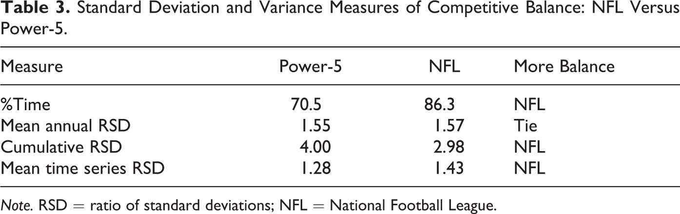
Note. RSD = ratio of standard deviations; NFL = National Football League.
The first metric, %Time, is the proportion of the overall league winning percentage variance (all teams, all years) that is accounted for by the variance of individual team winning percentages over the study period (Equation 3). A higher value of %Time indicates greater balance, that is, a higher proportion of the overall variance arising from year-to-year churning in league standings and/or a smaller proportion from within-season variation. The Power-5 value is 70.5% and NFL value is 86.3%, indicating less balance in the Power-5.
Next, in Table 3, are the competitive balance measures based on the normalized standard deviation of winning percentages (RSD). The second line of the table shows the 20-year mean annual RSD, the normalized mean of the annual standard deviations of winning percentages across league members. Lower annual RSD values indicate more balance within seasons. The mean annual RSDs for the Power-5 and the NFL are 1.55 and 1.57, respectively. The Power-5 RSD is only slightly less than the NFL, and the difference is not statistically significant. A standard difference-between-means test yields a t statistic of .60.
The third line of Table 3 reports the cumulative RSD, the normalized standard deviation of cumulative win percentages of league teams for the full study period. As with the annual RSD, a lower cumulative RSD value indicates more balance. The NFL’s cumulative RSD of 2.98 is lower than the Power-5’s value of 4.00, indicating less balance in the Power-5.
The last line of Table 3 shows the mean time series RSD for each league, that is, the mean of normalized individual team winning percentage standard deviations over the study period. A higher time series RSD value indicates greater variability in team winning percentages over time, more churning in league standings, and greater balance. The NFL’s time series RSD is higher than that for the Power-5, 1.43 versus 1.28, respectively, again implying less balance for the Power-5. The difference between the two means has a high degree of statistical significance, with a standard difference-between-means test yielding a t statistic of 3.23 (p = .0017).
Thus, three of the four winning percentage standard deviation or variance measures indicate better balance in the NFL compared to the Power-5, and the fourth indicates no difference between the two. Of particular note is the greater year-to-year churning in league standings among NFL teams. This of course is the opposite of the NCAA’s implied claim that moving toward a professional model would reduce competitive balance by increasing the dominance of leading programs.
Concentration metrics
We examine two competitive balance measures that focus on the concentration of team appearances over the 20-year study period in the top positions in league standings. The first is the N-HHI where larger values indicate greater concentration and less balance. The N-HHI, per Equation 7, is the amount by which HHI exceeds its minimum possible value, expressed as a percentage of its possible range.
The second concentration metric is the percentage of all league teams that are included in the top positions. A larger percentage indicates a greater variety of championship contenders, which in turn indicates better competitive balance. As noted above, to avoid statistical bias, we compare the top 5 and top 10 NFL positions to the top 10 and top 20 Power-5 positions, respectively. For the same reason, our “championship” comparison involves the NFL champion (the top 1 position) and the top 2 Power-5 positions.
Table 4 presents the results for the top position concentration competitive balance metrics. The “championship” top 2/1 concentration metrics are in the first two lines. The top 2/1 N-HHI is higher for the Power-5 at 12.9% versus 9.2% for the NFL, indicating greater concentration and lower competitive balance in the Power-5. Similarly, 37.5% of NFL teams won championships, as compared to 27.4% of Power-5 teams in the top 2 positions, also indicating lower balance in the Power-5.
CR Measures of Competitive Balance: NFL Versus Power-5.
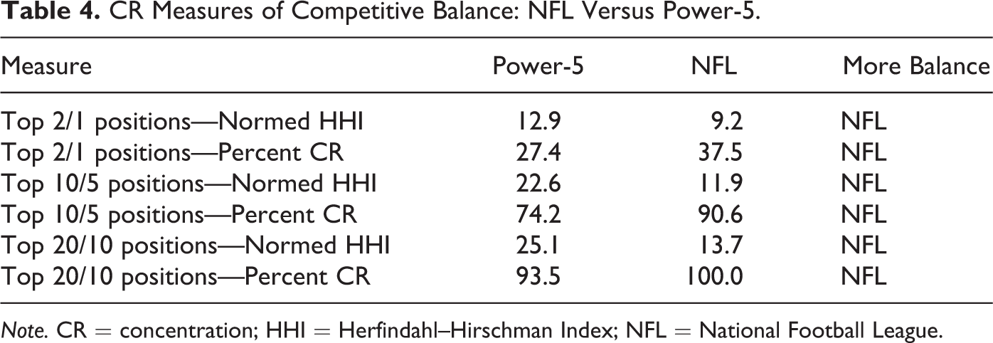
Note. CR = concentration; HHI = Herfindahl–Hirschman Index; NFL = National Football League.
The second two lines of Table 4 show the concentration metrics for the top 10 Power-5 positions and the top 5 NFL positions. For the Power-5, the top 10 N-HHI is 22.6%, almost twice the NFL’s top 5 value of 11.9%, indicating greater concentration and lower balance for the Power-5. Next, the Power-5 top 10 includes 74.2% of league teams compared to 90.6% for the NFL top 5, also indicating lower balance in the Power-5.
The third two lines of Table 4 show the concentration metrics for the top 20 Power-5 positions and the top 10 NFL positions. For the Power-5, the top 20 N-HHI is 25.1%, almost twice the NFL’s top 10 value of 13.7%, indicating greater concentration and lower balance for the Power-5. Next, the Power-5 top 20 includes 93.5% of league teams compared to 100.0% for the NFL top 10, also indicating lower balance in the Power-5.
Thus, all six position-related concentration metrics indicate that the Power-5 schools exhibit less balance than the NFL. Specifically, over the study period a smaller proportion of league teams dominated the championship competition. This is consistent with the lower level of churning in league standings reported above for the Power-5. As with the standard deviation and variance metrics, this is the opposite of the NCAA’s implied claim that a professional model yields lower competitive balance.
Summary and Conclusions
Over the last few decades, the NCAA’s Collegiate Model of athletic competition has become controversial as the revenues accruing to colleges and universities from top tier football and men’s basketball have increased dramatically. At the same time, athlete compensation has been stagnant, being limited to little more than the traditional athletic scholarship comprised mainly of tuition, room and board, and books. This increasingly conspicuous disparity has produced criticisms of the NCAA’s Collegiate Model. For example, many members of academia, the sports media and the public have called for significant increases in monetary compensation, arguing that athletes in the big money sports should receive a larger share of the revenue that they generate.
A key defense of its Collegiate Model proffered by the NCAA is that it promotes competitive balance. The implication is that a movement toward a professional model would tend to reduce balance. Of course, this hypothesis cannot be directly tested because the required counterfactual situations do not exist. The present article conducts an alternative test by comparing competitive balance in the top echelon of college football, essentially the so-called Power-5 conferences, to that for the professional NFL. We treat the college teams as a closed league, like the NFL, by excluding from their records all games against non-Power-5 opponents. Eight different albeit related competitive balance metrics are calculated for the NFL and Power-5 teams over the 1998-2017 study period.
The empirical analysis clearly indicates that the NFL’s competitive balance is not less than that of the Power-5 teams, contrary to the NCAA’s implied claims justifying its Collegiate Model. None of the eight metrics support this hypothesis. In fact, seven show better competitive balance in the NFL. Particularly notable is the relative dominance of leading teams in the Power-5 group, where there is less year-to-year churning in the standings and fewer teams occupying the top positions. Exploring the causal factors that underlie these results would be an interesting subject for future research. Be that as it may, the findings undermine competitive balance as a legitimate defense of the NCAA’s Collegiate Model, at a minimum imposing a substantial burden of proof.
Footnotes
Declaration of Conflicting Interests
The author(s) declared no potential conflicts of interest with respect to the research, authorship, and/or publication of this article.
Funding
The author(s) received no financial support for the research, authorship, and/or publication of this article.