kpsstest: A command that implements the Kwiatkowski,Phillips,Schmidt,and Shin test with sample-specific critical values and reports p-values

Abstract

Commonly used unit-root tests in time-series analysis—such as the Dickey–Fuller and Phillips–Perron tests—use a null hypothesis that the series contains a unit root. Such tests have low power against the alternative—when a time series is near integrated or highly autoregressive—implying that they do poorly in distinguishing such a series from having a unit root. Kwiatkowski et al. (1992, Journal of Econometrics 54: 159–178) introduced the Kwiatkowski, Phillips, Schmidt, and Shin test, in which the null hypothesis is that the series is stationary, to deal with this problem. One shortcoming of the presently available Kwiatkowski, Phillips, Schmidt, and Shin test in Stata is that it uses asymptotic critical values regardless of the sample size. This poses a problem in that researchers—especially social scientists—are often presented with short time series. I introduce kpsstest, a command that extends the previous implementation by including an option for a zero-mean-stationary null hypothesis, generating sample and test-specific critical values, and reporting appropriate p-values.

Keywords

st0671 kpsstest KPSS GKPSS unit-root tests stationary null hypothesis time series

1 Introduction

Commonly used unit-root tests in time-series analysis—such as the Dickey–Fuller and Phillips–Perron tests—are problematic because they perform poorly in distinguishing near-integrated or highly autoregressive series from unit roots. This implies that researchers, when presented with such series, would fail to conclude that these series are stationary when using the Dickey–Fuller and Phillips–Perron tests. That is, they would fail to reject the null hypothesis that the series contains a unit root. Failing to reject the null hypothesis does not necessarily imply that the null is true. It simply indicates that there exists an absence of strong evidence against the null hypothesis (Kwiatkowski et al. 1992).

To increase the information available to researchers about the time-series properties of their data, Kwiatkowski et al. (1992) introduced the Kwiatkowski, Phillips, Schmidt, and Shin (KPSS) test. The null hypothesis of the KPSS test is either that the series is trend stationary or that the series is level stationary. Kwiatkowski et al. (1992) recommended that the test be used in conjunction with unit-root tests whose null hypotheses are that the series contains a unit root. In their application, using economic time-series variables, Kwiatkowski et al. (1992) demonstrated that their test fails to reject the null hypothesis of stationarity and the Dickey–Fuller test fails to detect that the series are stationary. Thus, while researchers may use unit-root tests such as the Dickey–Fuller test, they should confirm their results with the KPSS test. This is especially important with highly autoregressive series, for which the Dickey–Fuller test has low power.

The KPSS test and its current implementation in Stata are wanting. Specifically, the implementation of the KPSS procedure uses asymptotic critical values—presented by Kwiatkowski et al. (1992, 166, table 1)—to test for significance of the KPSS test statistic. However, researchers are frequently presented with short time series or, at best, those that are unlikely to be considered infinite. Consequently, if the finite-sample distribution of the KPSS test statistic differs from its asymptotic distribution, then using asymptotic critical values with a finite sample poses threats to inference. A second shortcoming of the KPSS test and the current implementation of the test in Stata is the absence of a no-constant or zero-mean-stationary null hypothesis (Hobijn, Franses, and Ooms 2004). Third, while the current version of the KPSS test in Stata allows for the generalized Kwiatkowski, Phillips, Schmidt, and Shin (GKPSS) test, it does not provide GKPSS-specific critical values (Baum 2000). Finally, Baum’s (2000) kpss command does not provide users with p-values.

I introduce kpsstest to deal with these shortcomings. kpsstest provides users with finite-sample critical values from response surface regressions for any sample size between 10 and 400 observations for the KPSS and GKPSS tests and for all three null hypotheses options. For sample sizes larger than 400, kpsstest uses asymptotic critical values. Additionally, kpsstest uses the distribution of the KPSS test statistic for a given sample size to calculate p-values. Similar to kpss, kpsstest provides users with the option to implement either the original KPSS test or the GKPSS test (Hobijn, Franses, and Ooms 2004). kpsstest extends the capabilities of kpss by allowing users to implement the test against a null hypothesis of no constant or zero mean stationarity. Hobijn, Franses, and Ooms (2004) demonstrate that the distribution of this test statistic differs from the distribution of the test statistic when the null hypothesis is level stationary.

2 An overview of the KPSS test

2.1 The original KPSS test

In this section, I provide a brief overview of the original KPSS test developed by Kwiatkowski et al. (1992). A more technical description of the test can be found in the appendix. Consider a time series, y_t , with trend (t) and random-walk (r_t ) components, such that

\begin{array}{l} y_{t} = α + ξ t + d r_{t} + ε_{t}, where ε_{t} ~ N (0, σ_{ε}^{2}) \\ r_{t} = r_{t - 1} + u_{t}, where u_{t} ~ N (0, σ_{u}^{2}) \end{array}

where ξ_t are stationary errors. The kpss test is essentially a Lagrange multiplier test with a null hypothesis, $H_{o} : σ_{u}^{2} = 0$ , which means the series is stationary. Specifically, 1) when ξ is restricted to 0, the null hypothesis is that the series is level stationary; 2) when α, ξ, and d are all restricted to 0, the null hypothesis is that the series is zero mean stationary; and 3) when α, ξ, and d are not restricted to 0, the null hypothesis is that the series is trend stationary. Rejecting the null hypothesis means that the series is nonstationary and, if deemed necessary by the researcher, appropriate corrections (for example, differencing, or removing the trend) need to be made to account for the nonstationarity of the series.

2.2 The GKPSS test

Before I describe the GKPSS test, note that one step in calculating the KPSS test statistic requires estimating $σ_{\in}^{2}$ . And a component of the estimator of $σ_{\in}^{2}$ is the temporal dependence in the residuals—which needs to be weighted—from a regression of the series on a constant or on the trend term. For a zero-mean-stationary null hypothesis, the temporal dependence in the series itself needs to be weighted. To weight this temporal dependence, one needs to specify a kernel, w(). Using a kernel in this test also requires that one must specify the maximum number of lags of the residuals or series to be accounted for in the temporal dependence of residuals or series. This quantity is known as the lag truncation parameter. The original KPSS test uses a Bartlett kernel and a long or short Schwert criterion calculation to determine the appropriate lag truncation parameter. Readers interested in the technical description of these quantities may refer to the appendix. However, a technical understanding beyond the description in this paragraph is not necessary to understand the differences between the KPSS and GKPSS tests and which test to implement when testing for stationarity.

The GKPSS test builds on the KPSS test by using a different kernel and algorithm for calculating the lag truncation parameter (Hobijn, Franses, and Ooms 2004). The GKPSS test uses a quadric spectral kernel with an automatic bandwidth selection algorithm in determining the lag truncation parameter. The most important difference between the KPSS and GKPSS tests is realized in the statistical properties of the tests: although both tests are consistent, the GKPSS test has lower type 1 error rates than the KPSS test in finite samples.

2.3 Implementing the tests

The main differences between the KPSS and GKPSS tests are in the choice of kernel and the method in which the lag truncation parameter is determined. This leads to the question: which test should a researcher use?

As I mentioned, the KPSS test is found to have higher type 1 error rates for highly autoregressive series, whereas the GKPSS test, by using a quadratic spectral kernel and an automatic bandwidth selection algorithm for the lag truncation parameter, has a lower incidence of type 1 errors in finite samples (Hobijn, Franses, and Ooms 2004). Despite the superiority of the GKPSS test over the KPSS test, kpsstest allows users to implement the original KPSS test with a Bartlett kernel in combination with a userdefined lag truncation parameter, a short or long Schwert criterion, or an automatic bandwidth selection for selecting the lag truncation parameter.¹ Kwiatkowski et al. (1992, 170) used the Schwert criterion to select the lag truncation parameter because these were the choices being commonly made at the time. As Hobijn, Franses, and Ooms (2004) note about Kwiatkowski et al.’s (1992, 494) choice of the lag truncation parameter, “the automatic data dependent bandwidth selection procedure yields better small sample results than when the bandwidth is chosen arbitrarily, as by KPSS.” The user-defined lag truncation parameter option in kpsstest is for advanced practitioners who wish to implement the KPSS test with lags set manually. However, the literature demonstrates that the GKPSS test—that is, the KPSS test implemented with a quadratic spectral kernel and an automatic bandwidth selection algorithm for the lag truncation parameter—has the best statistical properties and should thus be preferred over other common implementations of the KPSS test.

With regard to the choice of the null hypothesis, kpsstest has three options: 1) zero mean stationary, 2) level stationary, and 3) trend stationary. A zero-mean-stationary null hypothesis [α = ξ = d = 0 in (1)] means that, under the null hypothesis, the series is stationary around a mean value of 0. A level-stationary null hypothesis implies that, under this null hypothesis, the series is stationary around a constant or drift term. Last, a trend-stationary null hypothesis means that a stationary series contains both a drift and a trend term. The Stata manual for dfuller (see [TS] dfuller) (Dickey– Fuller test) provides an excellent explanation for selecting which null hypothesis option to use. It suggests that the choice of null hypothesis must be theoretically or visually guided. If the user has a theory about the stationarity of a series, then the user may select the null hypothesis most suitable to that theory. However, more often than not a visual inspection of the series is preferred. If the user then finds a series to be trending upward or centered around zero, the user may select the trend-stationary or zero-meanstationary null hypothesis, respectively.

To summarize the above discussion, the GKPSS is the preferred test, and the choice of null hypothesis should largely focus on the visual inspection of the series.

3 Calculating sample-specific critical values and p-values

3.1 Response surface regressions and sample-specific critical values

Because response surface regressions easily provide accurate sample-specific critical values, I used this method to calculate critical values.² This involved the following steps:

For a given sample size, I simulated the distribution of the test statistic using 50,000 replications and calculated the 1, 2.5, 5, 7.5, 10, 12.5,…, 90, 95, 97.5, 99, 99.9, and 99.99 percentiles. Doing so provides the critical values of the test statistic at various levels of significance. For example, the critical value at the 0.01 significance level is the critical value at the 99 percentile.³

For the same sample size, I repeated this procedure 100 times and calculated the averages and standard deviations of the test statistics over the 100 experiments for each percentile.

I repeated the above two steps for the following 14 sample sizes: 10, 25, 50, 60, 75, 100, 125, 150, 200, 250, 300, 400, 500, and 2,000.

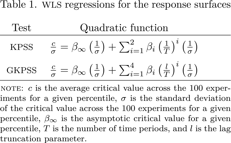
To account for heteroskedasticity, I fit a weighted least-squares (WLS) regression model for each percentile in which the average test statistic for each percentile is a quadratic function of time and the standard deviations for each percentile are used as weights (Davidson and MacKinnon 1993; MacKinnon 1994). The quadratic functions depend on the test used and are shown in table 1.

Table 1.

WLS regressions for the response surfaces

Test	Quadratic function
KPSS	$\frac{c}{σ} = β_{\infty} (\frac{1}{σ}) + \sum_{i = 1}^{2} β_{i} {(\frac{1}{T})}^{i} (\frac{1}{σ})$
GKPSS	$\frac{c}{σ} = β_{\infty} (\frac{1}{σ}) + \sum_{i = 1}^{4} β_{i} {(\frac{l}{T})}^{i} (\frac{1}{σ})$

note: c is the average critical value across the 100 experiments for a given percentile, σ is the standard deviation of the critical value across the 100 experiments for a given percentile, β_∞ is the asymptotic critical value for a given percentile, T is the number of time periods, and l is the lag truncation parameter.

Although the quadratic functions for these WLS models are determined through experimentation based on the best fit (R ² and sum of squared residuals), I use functional forms similar to those of Sephton (1995, 2017), who has demonstrated that such functional forms provide the most accurate estimates of the finite and asymptotic critical values for the KPSS and GKPSS tests. My results confirm that these functional forms provide the best-fitting regression models. The benefits of using response surface regressions are that—if the response surface is correctly specified—parameter estimates of the regressions can be used to calculate accurate sample-specific critical values with ease. The critical value $(\hat{c})$ for a particular sample size (T) can be approximated by substituting for T and the parameter estimates ( ${\hat{β}}_{_{\infty}}$ and $\sum_{i = 1}^{4} {\hat{β}}_{i}$ ) from the response surface regressions in the quadratic functions in table 1. Additionally, the fact that each data-generating process is subject to 50,000 replications and that this process is repeated 100 times reduces the experimental uncertainty involved in Monte Carlo experiments and increases the accuracy and precision of the estimates of quantities of interest (Davidson and MacKinnon 1993).⁴

3.2 Assessing the calculated critical values

The asymptotic critical values from my response surface regressions and those generated by Sephton (2017)—who also calculates KPSS and GKPSS critical values using response surface regressions—are compared in table 2. These results demonstrate that the asymptotic critical values, generated from response surface regressions for kpsstest, are similar to those generated by Sephton (2017). Similarly, the finite-sample critical values for the KPSS test with null hypotheses of level stationary and trend stationary are also similar to those generated by Sephton (2017).⁵ However, note that the finitesample critical values for the KPSS test with a null hypothesis of zero mean stationary and those for the GKPSS tests differ from Sephton (2017).

Table 2.

Comparison of asymptotic critical values

	KPSS			GKPSS
	10%	5%	1%	10%	5%	1%
	Zero mean stationary
kpsstest	1.197	1.655	2.788	1.198	1.658	2.797
Sephton (2017)	1.195	1.656	2.788	1.195	1.652	2.794
	Level stationary
kpsstest	0.347	0.461	0.744	0.347	0.461	0.742
Sephton (2017)	0.347	0.461	0.743	0.347	0.461	0.741
	Trend stationary
kpsstest	0.119	0.148	0.218	0.119	0.148	0.218
Sephton (2017)	0.119	0.148	0.218	0.118	0.146	0.218

While the finite-sample critical values generated by Sephton (2017) in smaller samples are sometimes four times as large as the asymptotic critical values, those used in kpsstest, for increases in sample size, demonstrate more gradual increments or decrements toward the asymptotic critical values. For example, while the asymptotic 1% critical value for the gkpss test with a zero-mean-stationary null hypothesis is between 2.79 and 2.80 (table 2), Sephton’s (2017) critical value is 9.477 for a sample size of 50. For the same sample size, the critical value I calculated from the response surface is 2.410. To confirm that the algorithm used in kpsstest generates the right critical values, I compared the test statistics, for a given time series, with those generated by Baum’s (2000) kpss command. I found the test statistics to be similar (as seen in section 4 of this article).⁶ Further, I conducted Monte Carlo experiments to analyze the type 1 error rates and power for tests in which our finite-sample critical values differed. I report results for the 5% significance level, at which a type 1 error rate of 0.05 and a power of 1 are expected.

Table 3 shows the type 1 error and power for the finite-sample critical values in kpsstest and for those in Sephton (2017). The type 1 error rates for kpsstest are either the same as or slightly above the type 1 errors for Sephton (2017), and they are almost always under the 0.05 expected value. The largest difference in type 1 error rates is for the GKPSS test with a trend-stationary null hypothesis for a time series of length 50. However, such a large difference is unusual for any other null hypothesis and sample size. When we compare power, the power gains in kpsstest are significantly higher, especially for the gkpss test with a zero-mean-stationary null hypothesis. Thus, overall with kpsstest, small losses in type 1 error rates are offset by large gains in power. However, with Sephton’s (2017) critical values, large losses in power are not offset by small gains in type 1 error rates.

Table 3.

Comparison of type 1 error rates and power between kpsstest and Sephton (2017)

		KPSS		GKPSS
		Zero mean	Zero mean	Level	Trend
		Type 1 error
T = 50	kpsstest	0.008	0.008	0.088	0.088
	Sephton (2017)	0.008	0.008	0.072	0.008
T = 75	kpsstest	0.024	0.024	0.048	0.048
	Sephton (2017)	0.016	0.000	0.040	0.024
T = 100	kpsstest	0.008	0.008	0.040	0.080
	Sephton (2017)	0.008	0.008	0.040	0.056
T = 200	kpsstest	0.032	0.032	0.072	0.016
	Sephton (2017)	0.024	0.024	0.072	0.016
		Power
T = 50	kpsstest	0.552	0.728	1	1
	Sephton (2017)	0.528	0.432	1	1
T = 75	kpsstest	0.632	0.640	1	1
	Sephton (2017)	0.624	0.512	1	1
T = 100	kpsstest	0.768	0.800	1	1
	Sephton (2017)	0.744	0.744	1	1
T = 200	kpsstest	0.872	0.896	1	1
	Sephton (2017)	0.856	0.896	1	1

3.3 Reported p-values

The 1, 2.5, 5, 7.5,…, 97.5, 99, 99.9, and 99.99 percentiles of the distributions of the test statistics correspond to p-values of 0.99, 0.975, 0.95, 0.925,…, 0.025, 0.01, 0.001, and 0.0001, respectively. When the test statistic is equal to the critical value (up to four decimal places) for the calculated percentiles, kpsstest reports the corresponding p-value. When the test statistic is less than the 1 percentile value of the distribution, kpsstest reports a p-value of 1. When the test statistic lies between the 1 percentile and 99.99 percentile values of the distribution and is not equal to a critical value for the calculated percentiles, kpsstest linearly interpolates the p-value.⁷ Finally, when the test statistic is greater than the 99.99 percentile value of the distributions, kpsstest reports a p-value of 0.00001.⁸

4 Syntax

kpsstest varname [if] [in] , [[kpss| gkpss]

[ trunclag(string)| lag(#)| auto] [noconstant| level| trend ]]

varname is the variable to be tested for stationarity using the kpss or gkpss test. If no options are specified, the gkpss test with a zero-mean-stationary null hypothesis is conducted by default.

5 Options

kpss indicates that a Bartlett kernel will be used to weight the serial dependence in the residuals when calculating the estimate of the long-run variance and will be used in conjunction with a Schwert criterion, a user-specified value, or an automatic bandwidth selection for the lag truncation parameter. trunclag(), lag(), or auto must be specified with the kpss option.

gkpss indicates that a quadratic spectral kernel will be used to weight the serial dependence in the residuals when calculating the estimate of the long-run variance in conjunction with automatic bandwidth selection to determine the lag truncation parameter. Except for the choice of the null hypothesis, no other option is allowed when specifying gkpss. If the user specifies neither kpss nor gkpss, gkpss is used by default.

trunclag(string) indicates that the Schwert criterion will be used to calculate the lag truncation parameter for the kernel. Users will specify either short or long. This option can be used only with the kpss option.

lag(#) allows the user to specify the lag truncation parameter to be used in the Bartlett kernel. This option can be used only with the kpss option.

auto indicates automatic bandwidth selection for the lag truncation parameter is to be used in the Bartlett kernel. This option can be used only with the kpss option.

noconstant indicates that a zero-mean-stationary null hypothesis will be used. This is the default option if a null hypothesis is not specified. This option may not be used with level or trend.

level indicates that a level-stationary null hypothesis will be used. This option may not be used with noconstant or trend.

trend indicates that a trend-stationary null hypothesis will be used. This option may not be used with noconstant or level .

The two types of tests (kpss and gkpss) that kpsstest can implement, combined with the various lag truncation parameter options and the three null hypotheses options, can make implementing kpsstest confusing. To aid with implementing the command, figure 1 demonstrates how a practitioner can use kpsstest . First, the user must specify kpsstest varname, followed by the choice of whether the user wants to use the kpss or gkpss test. If the user chooses kpss, then the user must choose between trunclag() , lag() , or auto for determining the lag truncation parameter. The user must then select the null hypothesis (for example, kpsstest varname, kpss auto level ). If the user chooses gkpss, then the user needs to only select the null hypothesis (for example, kpsstest varname, gkpsstrend ). If the user chooses no option at all, a gkpss test with a zero-mean-stationary null hypothesis is conducted by default (for example, kpsstest varname).

Figure 1.

Using kpsstest with its various options

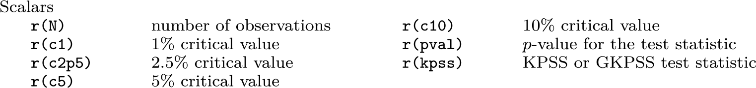
5.1 Stored results

kpsstest stores the following in r():

6 Examples

In this section, I demonstrate the utility of kpsstest using examples. First, I demonstrate its similarities to Baum’s (2000) kpss command; second, how kpsstest extends the capabilities of kpss and provides more functionality to the user; and finally, how users can use a visual inspection of the series to appropriately select the null hypothesis and the implications of failing to do so.

6.1 Similarities between kpss and kpsstest for the gkpss test

The first example is a stationarity test for the log of consumption from the German macroeconomic data (Lütkepohl 1993) available in Stata. I implement the gkpss test (kpss test with a quadratic spectral and automatic bandwidth selection procedure) using both kpss and kpsstest for a trend-stationary null hypothesis.

As seen above, Baum’s (2000) kpss command finds that the automatic bandwidth selection algorithm selects a lag truncation parameter of 3 and finds the test statistic to be 0.232.

Similar to kpss, kpsstest determines the lag truncation parameter to be 3 and displays a test statistic of 0.232. However, kpsstest displays sample-specific gkpss test critical values, while kpss displays asymptotic kpss test critical values. The output of kpsstest is also more user friendly. This output should be familiar to Stata users because it mimics that of the Dickey–Fuller test (dfuller). It neatly displays the number of observations, the test statistic, and the critical values. In contrast to kpss, kpsstest displays the p-value for the given test statistic, saving users time from having to identify the significance of the test statistic by comparing the test statistic with the critical values.

6.2 Similarities between kpss and kpsstest for the kpss test

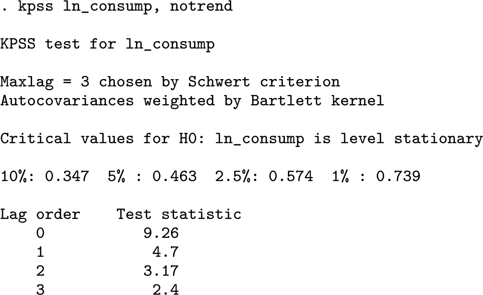
In this example, using the same macroeconomic data as the previous example, I compare the functionality of kpss and kpsstest for the original kpss test—with a Bartlett kernel and Schwert criterion for a short lag truncation parameter—with a level-stationary null hypothesis.

As seen above, Baum’s (2000) kpss command determines the short lag truncation parameter to be 3 and finds the test statistic at the third lag to be 2.4.

kpsstest concludes similarly to kpss with two differences. First, kpss returns the test statistic for every lag up to the third lag. While there is no ex ante reason to do so, users of kpsstest may recover similar output using the lag() option. Second, the test statistic from kpss at the third lag is 2.4, while that from kpsstest is 2.404. This is because the test statistic from kpss is rounded to one decimal place and that from kpsstest is rounded to three decimal places. The test statistics without rounding for kpss and kpsstest are similar up to six decimal places.

6.3 Similarities between kpss and kpsstest for a user-defined lag truncation parameter

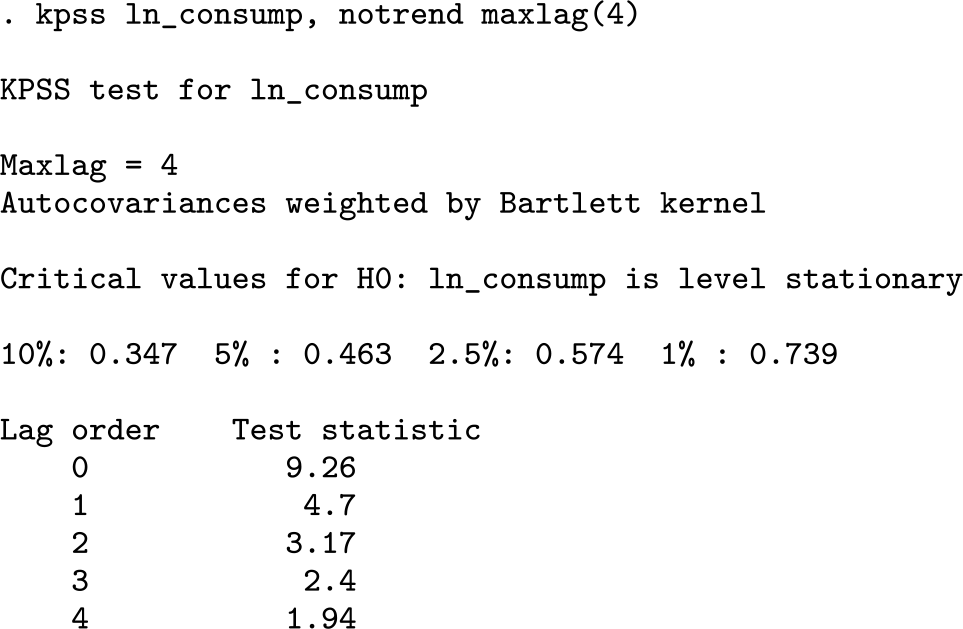
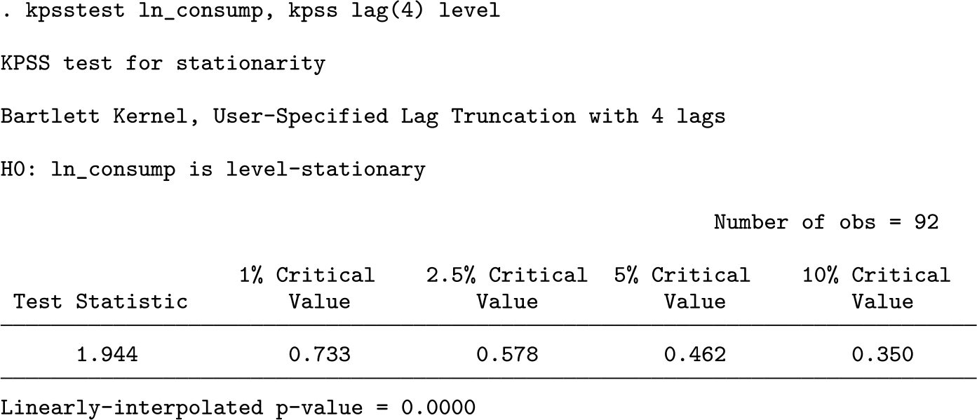
Continuing with the same German macroeconomic data as in the previous examples, I now compare the results from kpss and kpsstest for the original kpss test with a user-defined lag truncation parameter (4 for this example).

As shown in the above output, Baum’s (2000) kpss command returns a test statistic of 1.94 at the fourth lag.

kpsstest also returns a similar test statistic (1.944) but rounded to the three decimal places instead of two as in kpss. The test statistics are identical up to six decimal places.

6.4 Similarities between kpss and kpsstest for automatic bandwidthselected lag truncation parameter

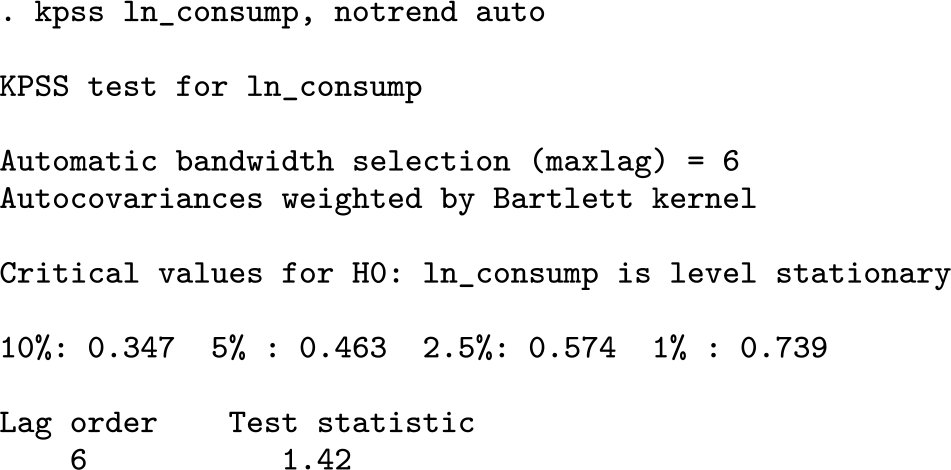
Using the same time series as above, the examples below compare the results from kpss and kpsstest for the original kpss test with a Bartlett kernel used in conjunction with the automatic bandwidth selection criterion in determining the lag truncation parameter.

As seen above, Baum’s (2000) kpss command calculates the lag truncation parameter to be equal to 6, which results in a test statistic of 1.42.

kpsstest recovers a similar test statistic equal to 1.419 after determining the lag truncation parameter is 6.⁹ The test statistics from both kpsstest and kpss are identical up to 6 decimal places.

So far, while we have looked at the similarities between the two commands in terms of test statistics and functionality, we have also noted differences: 1) kpsstest‘s output is user friendly, resembling that of dfuller; and 2) kpsstest displays the number of observations, the sample-specific critical values, and the p-value for the test statistic. The next few examples will demonstrate other ways in which kpsstest differs from kpss.

6.5 kpsstest with a zero-mean-stationary null hypothesis

kpss lacks the feature that allows for a zero-mean-stationary null hypothesis for the original kpss and gkpss tests. Using the same German macroeconomic data as in the above examples, I demonstrate how users can implement the gkpss test with a zero-mean-stationary null hypothesis using kpsstest.

The above output demonstrates that the gkpss test for log of consumption rejects the null hypothesis that the series is zero mean stationary. This means that the test rejects that the series is stationary when we do not account for constant and trend terms.

6.6 kpsstest with a Schwert criterion and long lag truncation parameter

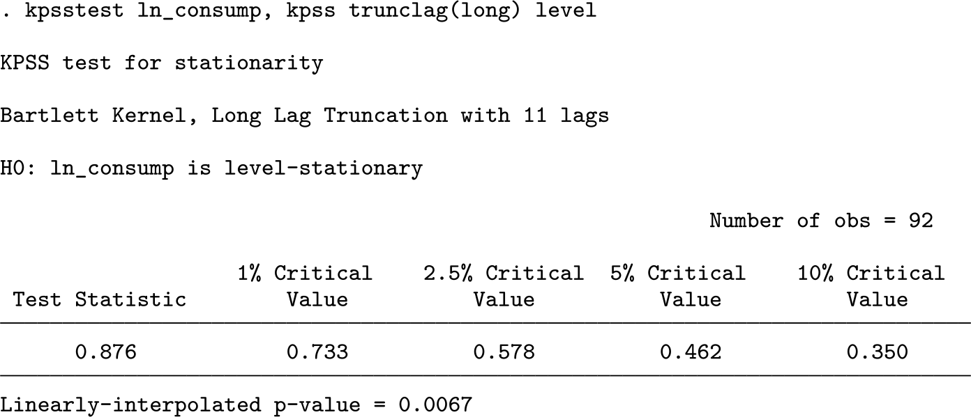
In calculating the lag truncation parameter using a Schwert criterion for the Bartlett kernel in the original kpss test in addition to the trunclag(short) and lag() options, users may specify the trunclag(long) option when using kpsstest. This was one of the options used by Kwiatkowski et al. (1992). kpss does not allow for this option. I demonstrate how users may do so using the log of consumption from the German macroeconomic dataset used above for a level-stationary null hypothesis.

The results demonstrate that the lag truncation parameter is determined to be 11 using a long Schwert criterion. The test rejects the null hypothesis that the series is level stationary.

6.7 Choosing a null hypothesis for kpsstest

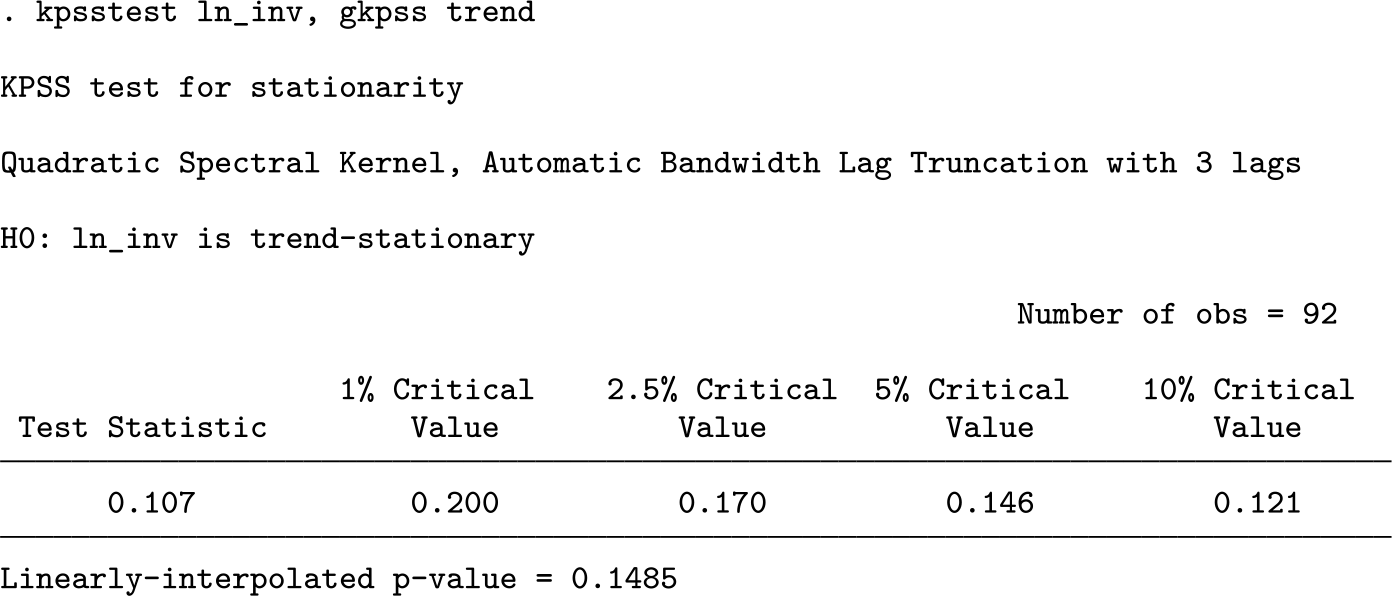
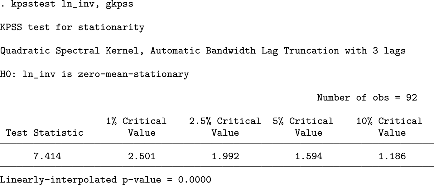
As mentioned earlier in the article, kpsstest provides users with the choice of a zero-mean-stationary, level-stationary, or trend-stationary null hypothesis. This choice should be guided by theory, if possible, but should largely be a consequence of visual inspection of the time series. Consider the log of investment, plotted in figure 2, using the same German macroeconomic data as in the previous examples.

Figure 2.

Time-series line plot for the log of investment

The above figure clearly demonstrates that the log of investment is trending upward over time. This suggests that a trend-stationary null hypothesis is appropriate. Failing to use a trend-stationary hypothesis could lead to the conclusion that the series is nonstationary and may contain a unit root when the series is actually trend stationary.

As seen in the output above, the choice of a gkpss test with a trend-stationary null hypothesis finds that the series is indeed trend stationary. While the gkpss tests with the other null hypotheses, as seen in the two examples below, may correctly provide insight that the series is nonstationary, they can lead to the false inference that this nonstationarity is due to a unit root.

This example demonstrates that a visual inspection of a series is insightful and necessary to determine the choice of null hypothesis. It also demonstrates that using the incorrect null hypothesis can lead to incorrect inferences about the stationarity of the series.

7 Conclusion

In this article, I briefly described the kpss test and later extensions to the test. I introduced a command—kpsstest—that can implement the original kpss and the gkpss tests. kpsstest also provides users with sample and test-specific critical values and p-values for the test statistic. Thus, kpsstest offers users more appropriate inferences and the ability to easily interpret the test’s result through a p-value. Users would otherwise have to check for the test statistic’s statistical significance by determining whether the test statistic lies above, between, or below the asymptotic critical values provided by Kwiatkowski et al. (1992). As Sephton (2017) demonstrates, using asymptotic critical values for finite samples is inappropriate and can lead to incorrect inferences. Additionally, kpsstest allows for a null hypothesis that the series has no constant or is zero mean stationary.

Supplemental Material

Supplemental Material, sj-zip-1-stj-10.1177_1536867X221106371 - kpsstest: A command that implements the Kwiatkowski, Phillips, Schmidt, and Shin test with sample-specific critical values and reports p-values

Supplemental Material, sj-zip-1-stj-10.1177_1536867X221106371 for kpsstest: A command that implements the Kwiatkowski, Phillips, Schmidt, and Shin test with sample-specific critical values and reports p-values by Ali Kagalwala in The Stata Journal

Footnotes

Notes

8 Acknowledgments

Portions of this research were conducted with the advanced computing resources and consultation provided by Texas A&M High Performance Research Computing. The author thanks the editor, the anonymous reviewer, Peter Sephton, and Guy D. Whitten for their useful comments and suggestions.

9 Programs and supplemental materials

To install a snapshot of the corresponding software files as they existed at the time of publication of this article, type

A Appendix

References

Andrews

D. W. K.

1991. Heteroskedasticity and autocorrelation consistent covariance matrix estimation. Econometrica 59: 817–858. https://doi.org/10.2307/2938229.

Baum

C. F.

2000. kpss: Stata module to compute Kwiatkowski–Phillips–Schmidt–Shin test for stationarity. Statistical Software Components S410401, Department of Economics, Boston College. https://ideas.repec.org/c/boc/bocode/s410401.html.

Davidson

MacKinnon

J. G.

1993. Estimation and Inference in Econometrics. New York: Oxford University Press.

Engle

R. F.

Hendry

D. F.

Trumble

1985. Small-sample properties of ARCH estimators and tests. Canadian Journal of Economics 18: 66–93. https://doi.org/10.2307/135114.

Ericsson

N. R.

1991. Monte Carlo methodology and the finite sample properties of instrumental variables statistics for testing nested and non-nested hypotheses. Econometrica 59: 1249–1277. https://doi.org/10.2307/2938367.

Hendry

D. F.

1979. The behavior of inconsistent instrumental variables estimators in dynamic systems with autocorrelated errors. Journal of Econometrics 9: 295–314. https://doi.org/10.1016/0304-4076(79)90076-9.

Hobijn

Franses

P. H.

Ooms

2004. Generalizations of the kpss-test for stationarity. Statistica Neerlandica 58: 483–502. https://doi.org/10.1111/j.1467-9574.2004.00272.x.

Kwiatkowski

Phillips

P. C. B.

Schmidt

Shin

1992. Testing the null hypothesis of stationarity against the alternative of a unit root: How sure are we that economic time series have a unit root? Journal of Econometrics 54: 159–178. https://doi.org/10.1016/0304-4076(92)90104-Y.

Lütkepohl

1993. Introduction to Multiple Time Series Analysis. 2nd ed. New York: Springer.

10.

MacKinnon

J. G.

1994. Approximate asymptotic distribution functions for unit-root and cointegration tests. Journal of Business and Economic Statistics 12: 167–176. https://doi.org/10.2307/1391481.

11.

Newey

W. K.

West

K. D.

1994. Automatic lag selection in covariance matrix estimation. Review of Economic Studies 61: 631–653. https://doi.org/10.2307/2297912.

12.

Sephton

P. S.

1995. Response surface estimates of the kpss stationarity test. Economics Letters 47: 255–261. https://doi.org/10.1016/0165-1765(94)00561-F.

13.

Sephton

P. S.

. 2017. Finite sample critical values of the generalized kpss stationarity test. Computational Economics 50: 161–172. https://doi.org/10.1007/s10614-016-9586-z.

14.

Trapletti

Hornik

LeBaron

2019. tseries: Time series analysis and computational finance. R package version 0.10–49. http://cran.r-project.org/web/packages/tseries/.

15.

Vega Yon

G. G.

Quistorff

2019. parallel: A command for parallel computing. Stata Journal 19: 667–684. https://doi.org/10.1177/1536867X19874242.

Supplementary Material

Please find the following supplemental material available below.

For Open Access articles published under a Creative Commons License, all supplemental material carries the same license as the article it is associated with.

For non-Open Access articles published, all supplemental material carries a non-exclusive license, and permission requests for re-use of supplemental material or any part of supplemental material shall be sent directly to the copyright owner as specified in the copyright notice associated with the article.

0.62 MB

0.00 MB