Panel stochastic frontier models with endogeneity

Abstract

In this article, I introduce xtsfkk as a new command for fitting panel stochastic frontier models with endogeneity. The advantage of xtsfkk is that it can control for the endogenous variables in the frontier and the inefficiency term in a longitudinal setting. Hence, xtsfkk performs better than standard panel frontier estimators such as xtfrontier that overlook endogeneity by design. Moreover, xtsfkk uses Mata’s moptimize() functions for substantially faster execution and completion speeds. I also present a set of Monte Carlo simulations and examples demonstrating the performance and usage of xtsfkk.

Keywords

st0686 xtsfkk panel stochastic frontier models longitudinal data endogeneity production frontier cost frontier endogenous inefficiency

1 Introduction

It has been more than 40 years since Aigner, Lovell, and Schmidt (1977) and Meeusen and van den Broeck (1977) introduced stochastic frontier models. These models are composed of a deterministic part identifying the frontier goal, a stochastic part for the two-sided error term, and a one-sided inefficiency error term identifying the distance from the stochastic frontier. They can be used to study production, cost, revenue, profit, or other goals within various industries. Over the years, these models have become quite common in the literature as empirical researchers have applied them in their research articles and theoretical researchers have modified them to address further needs. Kumbhakar and Lovell (2000) review this literature and summarize numerous applications of these models in many different industries, such as accounting, advertising, banks, education, financial markets, environment, hospitals, hotels, labor markets, military, police, real estate, sports, transportation, and utilities.

Stata provides the frontier command to estimate the parameters of a stochastic frontier model. Petrin, Poi, and Levinsohn (2004) offer a new command called levpet to estimate production functions using the econometric methodology of Levinsohn and Petrin (2003). Yasar, Raciborski, and Poi (2008) offer another command called opreg to estimate production functions with selection bias or simultaneity by implementing the methodology of Olley and Pakes (1996). Amadou (2012) provides the frontierhtail command to fit stochastic frontier models with fat tails as outlined by Gupta and Nguyen (2010). Belotti et al. (2013) introduce a command called sfcross that mirrors Stata’s frontier command with additional functionality, options, and models. Fé and Hofler (2020) provide a new command called sfcount that fits cross-sectional stochastic frontier models with a dependent count variable in the style of Fé and Hofler (2013).

However, the literature on stochastic frontier models, various commands, and the estimator options in other general-purpose statistical software packages does not offer a way to control for endogeneity that can exist in these models. If the determinants of the frontier or the inefficiency term are correlated with the two-sided error term of the model, then the outcomes of the standard estimators would be contaminated by endogeneity. Intrigued by this shortage in the literature, Kutlu (2010) addresses the endogeneity issue in stochastic frontier models in his article. Karakaplan and Kutlu (2017a) develop a model to handle endogeneity due to the determinants of the frontier or the inefficiency term, or both. Furthermore, Karakaplan (2017) offers a new command called sfkk to make it easy for researchers to analyze empirical stochastic frontier models with endogeneity. As a result of these efforts, many research articles such as Xu and Chen (2018), Germeshausen, Panke, and Wetzel (2020), and Karakaplan and Kutlu (2019) applied these methodologies and published various empirical findings.

Karakaplan and Kutlu (2017a) and the sfkk command of Karakaplan (2017) are designed to be cross-sectional. Karakaplan and Kutlu (2017b), on the other hand, design a stochastic frontier estimator that would resolve endogeneity issues in a panel setting. The standard xtfrontier command of Stata and sfpanel command of Belotti et al. (2013) fit panel stochastic frontier models but ignore the endogeneity issues identified by Karakaplan and Kutlu (2017b). Therefore, in this article, I introduce a new command, xtsfkk, for fitting panel stochastic frontier models with endogeneity in Stata.

2 The model

Karakaplan and Kutlu (2017b) present the following panel stochastic frontier model with endogenous explanatory variables in the frontier and inefficiency terms (for full model, see Karakaplan and Kutlu [2017b]):

\begin{array}{l} \ln L_{i} = \ln L_{i, y ∣ x} + \ln L_{i, x} \\ \ln L_{i, y ∣ x} = - \frac{1}{2} {T_{i} \ln (2 π σ_{w}^{2}) + \frac{e_{i .}^{'} e_{i .}}{σ_{w}^{2}} + (\frac{μ^{2}}{σ_{u}^{2}} - \frac{μ_{i *}^{2}}{σ_{i *}^{2}})} + \ln {\frac{σ_{i *} Φ (\frac{μ_{i *}}{σ_{i *}})}{σ_{u} Φ (\frac{μ}{σ_{u}})}} \\ \ln L_{i, x} = - \frac{1}{2} \sum_{t = 1}^{T_{i}} {\ln (| 2 π Ω |) + ϵ_{i t}^{'} Ω^{- 1} ϵ_{i t}} \\ μ_{i *} = \frac{σ_{w}^{2} μ - s σ_{u}^{2} e_{i .}^{'} h_{i .}}{σ_{u}^{2} h_{i .}^{'} h_{i .} + σ_{w}^{2}} \\ σ_{i *}^{2} = \frac{σ_{u}^{2} σ_{w}^{2}}{σ_{u}^{2} h_{i .}^{'} h_{i .} + σ_{w}^{2}} \\ e_{i t} = y_{i t} - x_{1 i t}^{'} β - ϵ_{i t}^{'} η \\ ϵ_{i t} = x_{i t} - Z_{i t} δ \end{array}

where a vector of observations corresponding to the panel i is represented by a subscript i.; T_i is the number of time periods for panel i; s = 1 for cost functions or s = −1 for production functions; y_it is the logarithm of the production or cost of the ith productive unit at time t; x _yit is a vector of exogenous and endogenous variables; x _it is a vector of all endogenous explanatory variables; $Z_{i t} = I_{p} \otimes z_{i t}^{'}$ where z _it is a vector of all exogenous variables; v _it and $ϵ_{i t}$ are two-sided error terms; u_it ≥ 0 is a one-sided error term capturing inefficiency; $h_{i t} = h ({x^{'}}_{u i t} φ_{u}) > 0;$ x _uit is a vector of exogenous and endogenous variables excluding the constant; $u_{i}^{*}$ is a producer-specific random component independent from v _it and $ϵ_{i t}$ ; Ω is the variance–covariance matrix of $ϵ_{i t}$ ; $σ_{v}^{2}$ is the variance of v _it ; ρ is the vector representing correlation between ${\tilde{ϵ}}_{i t}$ and v _it ; $w_{i t} = σ_{v} \sqrt{1 - ρ^{'} ρ} {\tilde{W}}_{it} = σ_{ω} {\tilde{W}}_{it};$ $η = σ_{w} Ω^{- 1 / 2} ρ / \sqrt{1 - ρ^{'} ρ;}$ e_it is conditionally independent from the regressors given x _it and z _it ; Φ denote the standard normal cumulative distribution function; $u_{i}^{*} \sim N^{+} (μ, σ_{u}^{2})$ (N⁺ is standard notation for half-normal distribution); and $h_{i t}^{2} = \exp ({x^{'}}_{u i t} φ_{u}) .$ Karakaplan and Kutlu (2017b) provide all the details about assumptions and how they derived the estimator.

Furthermore, to predict efficiency, Eff _it = exp(−u _it ), Karakaplan and Kutlu (2017b) give the following formula:

\exp {- E (u_{i t} ∣ e_{i})} = \exp [- h_{i t} {μ_{i *} + \frac{σ_{i *} ϕ (\frac{μ_{i *}}{σ_{i *}})}{Φ (\frac{μ_{i *}}{σ_{i *}})}}]

where ϕ denotes the standard normal probability distribution function.

Finally, Karakaplan and Kutlu (2017b) offer a test for endogeneity based on a reasoning similar to that of the standard Durbin–Wu–Hausman test. The test here is conducted by looking at the joint significance of the components of the η term. If the components of the η term are jointly significant, then that would tell us there is endogeneity in the model and a correction through (1) would be needed. If, on the other hand, the joint significance of the components is rejected, then correction for endogeneity would not be needed and the model can be fit by traditional frontier models.

3 The xtsfkk command

Using Mata’s maximum-likelihood estimator tools (the moptimize() functions), and the exceptional guidance provided by Gould, Pitblado, and Poi (2010) and Kumbhakar, Wang, and Horncastle (2015), I programmed the xtsfkk command, which can calculate (1) and (2). There are two files that are included in the xtsfkk command package: xtsfkk.ado, containing the main estimation syntax and the evaluator subroutines that xtsfkk calls behind the scenes, and xtsfkk.sthlp, containing helpful information about the command, which users can access by typing help xtsfkk in Stata. All front-end interaction with xtsfkk and most postestimation routines, including the output style, efficiency prediction, and endogeneity tests, are carried by the xtsfkk.ado file. The main evaluator subroutine runs with method d0, which calculates the overall log likelihood. Finally, the unabridged versions of the subsequent sections on syntax, options, and stored results are available in the xtsfkk help file.

3.1 Estimation syntax and options

Below is an abridged list of the options provided by xtsfkk presenting the most important features of the command. Users can type help xtsfkk in Stata for the full-length documentation of the xtsfkk syntax, options, stored results, and other details.

3.1.1 Syntax

xtsfkk depvar [indepvars] [if] [in] [weight] [, options]

pweights, aweights, fweights, and iweights are allowed; see [U] 11.1.6 weight.

3.1.2 Options

See the help file for a full list of options.

production specifies that the model be fit as a production frontier model. This option is the default and thus may be omitted.

cost specifies that the model be fit as a cost frontier model.

endogenous(endovarlist) specifies that the variables in endovarlist be treated as endogenous. By default, xtsfkk assumes that the model is exogenous.

instruments(ivarlist) specifies that the variables in ivarlist be used as instrumental variables (IVs) to handle endogeneity. By default, xtsfkk assumes that the model is exogenous.

uhet(uvarlist [, noconstant ] ) specifies the inefficiency component is heteroskedastic, with the variance function depending on a linear combination of uvarlist. Specifying noconstant suppresses the constant term from the variance function.

whet(wvarlist) specifies that the idiosyncratic error component is heteroskedastic, with the variance function depending on a linear combination of wvarlist.

header displays a summary of the model constraints in the beginning of the regression. header provides a way to check the model specifications quickly while the estimation is running or a guide to distinguish different regression results that are kept in a single log file.

compare fits the specified model with the exogeneity assumption and displays the regression results after displaying the endogenous model regression results.

efficiency(effvar [, replace ] ) generates the production or cost efficiency variable effvar_EN once the estimation is completed and displays its summary statistics in detail. Notice that the option automatically extends any specified variable name effvar with _EN. If the compare option is specified, the efficiency() option also generates effvar_EX, the production or cost efficiency variable of the exogenous model, and displays its summary statistics. Specifying replace replaces the contents of the existing effvar_EN and effvar_EX with the new efficiency values from the current model.

test provides a method to test the endogeneity in the model. test tests the joint significance of the components of the eta term and reports the findings after displaying the regression results. For more information about test, see Karakaplan and Kutlu (2017b).

nicely displays the regression results nicely in a single table. nicely uses estout, a community-contributed command by Jann (2005), to format some parts of the table, and xtsfkk table style resembles that of Karakaplan and Kutlu (2017b). The nicely option checks whether the estout package is installed on Stata, and if not, then the nicely option installs the package. If the compare option is specified along with nicely, then the table displays the exogenous and endogenous models with their corresponding equations and statistics side by side in a single table for easy comparison. nicely estimates the production or cost efficiency and tests endogeneity, and reports them in the table even if the efficiency() or test option is not specified.

Two unique functionalities that come with xtsfkk are save() /load() and beep:

save(filename) saves the current status of the estimation to the hard drive in every iteration while the estimation is running. Saving is especially useful if the user thinks that intentional breaks may be needed or unintentional interruptions (such as a power outage) may happen while the estimation is running. The save() option allows stopping the estimation temporarily to release memory for other tasks, and then continuing from where the estimation was left by using the load() option. Even if the computer completely shuts down for some external reason, as long as the save() option is specified, the estimation can continue from where it was with use of the load() option.

load(filename) loads the estimation from a previously saved file to continue from where the estimation was. The model specification with the load() option needs to be the same as the specification in the saved file. The save() and load() options use matin4-matout4 by Baum and Gould (2004).

beep [ (#) ] is useful for multitasking. beep produces a single beep when xtsfkk reports all the findings. When beep(#) is specified with a positive number, it produces # beeps when the results are ready. If # is a negative number, then beep acts like an alarm and produces continuous beeps until the user stops them. With the beep option, the user would not need to constantly monitor the Stata Results window for the outcome. Instead, the user can do other things until the computer starts beeping. This functionality is especially useful if the model is complicated and the panel dataset is large so that the estimation may take hours to complete, and the user wants to know when the outcome is ready.

4 Monte Carlo simulations

I implement Monte Carlo simulations to examine the performance of xtsfkk. I analyze three simulation scenarios in three tables: table 1 is for the effects of different panel data sizes; table 2 is for the effects of different IV strengths; and table 3 is for the effects of different degrees of endogeneity. Without loss of generality, I set up the scenarios as cost models, and put one endogenous variable (z₁) in the frontier and one endogenous variable (z₂) in the cost inefficiency. The setting and the data-generation process are summarized below:

\begin{array}{l} y = β_{c 1} + β_{x 1} x_{1} + β_{z 1} z_{1} + u + v \\ σ_{u}^{2} = \exp (β_{c 2} + β_{x 2} x_{2} + β_{z 2} z_{2}) \\ u^{*} ~ N^{+} (0, 1) \\ u = σ_{u} u^{*} \end{array}

where x₁ and x₂ are exogenous variables, and z₁ and z₂ are endogenous variables. In the true model, all coefficients are set to 0.5, and all variables are generated randomly from the normal distribution with a mean of 0 and a standard deviation of 1. I use the gentrun command by Wang (1999) to create u^∗. The endogeneity of z₁ and z₂ are independently and randomly generated from the normal distribution with a mean of v × ϱ and a standard deviation of 1 − ϱ where the degree of endogeneity increases with the ϱ parameter. The IVs iv₁ and iv₂ are also independently and randomly generated from the normal distribution with a mean of z₁ × δ and z₂ × δ, respectively, and a standard deviation of 1 − δ, where the strength of IVs increases with the δ parameter.

I use the psimulate2 parallel simulation command in the simulate2 package by Ditzen (2019) to run the Monte Carlo simulations with 500 repetitions each. All tables present average estimated coefficients, mean squared errors (MSE) of the estimated coefficients, mean and median cost efficiency scores, MSEs of the cost efficiency scores, and Pearson and Spearman correlations between cost efficiency scores of the true model and the analyzed model. Model EX is the model that ignores endogeneity, and model EN is the model that handles endogeneity.

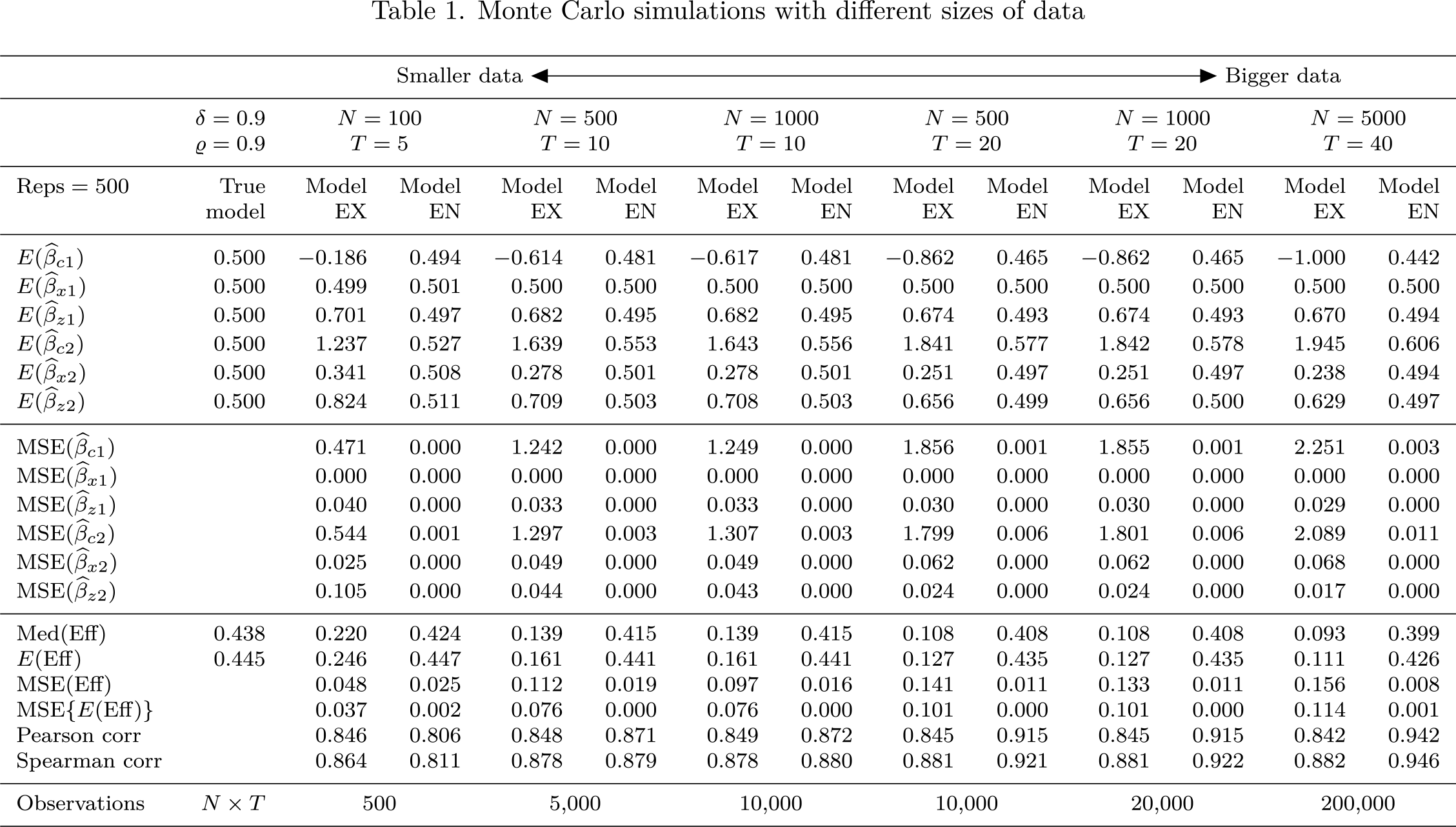
Table 1 presents the simulation results with different data sizes ranging from 500 to 200,000 observations. The number of individual productive units, N, ranges from 100 to 5,000, and the number of time periods, T, ranges from 5 to 40. Additionally, ϱ and δ are set to 0.9 (high endogeneity and strong IVs). Compared with model EX, model EN’s average coefficient estimates are more similar to the true model in all columns of table 1, and the coefficient MSEs of model EN are mostly smaller than that of model EX. In terms of cost efficiency scores, model EN seems to perform better as the size of the data increases. When T is too small (T < 8), Pearson and Spearman correlations of model EN start dropping below that of model EX. However, the MSEs of the efficiency scores are still smaller in model EN when T = 5. Table 1 provides an impression that, with different sizes of data, model EN generally performs better than model EX.

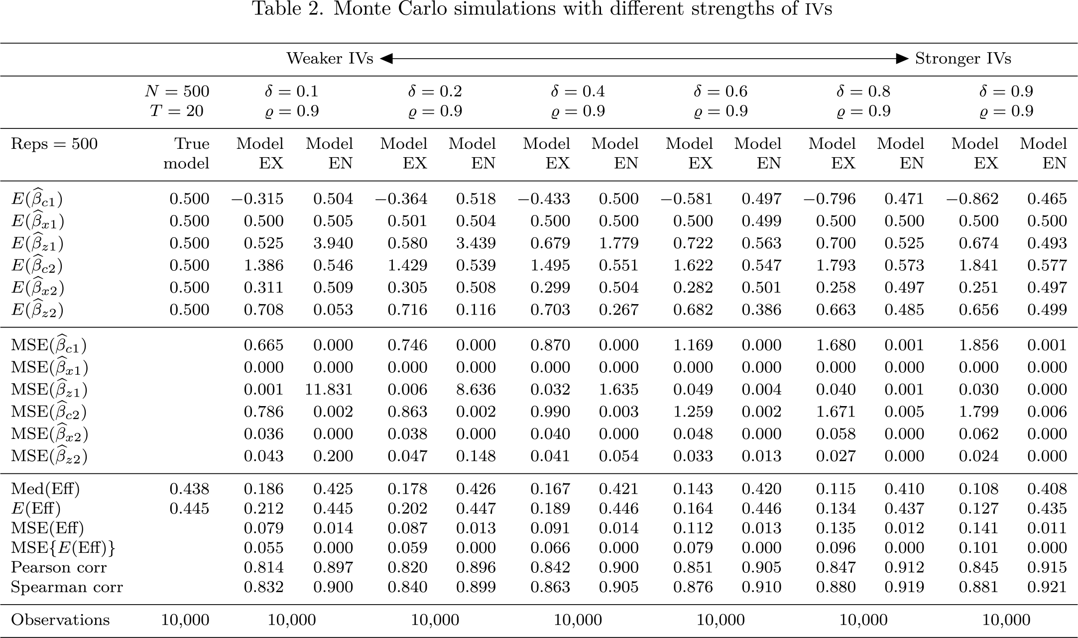
In table 2, the simulation results are presented with different strengths of IVs, with ϱ set to 0.9 (high endogeneity), N set to 500, and T set to 20. This table demonstrates that with stronger IVs (δ > 0.6), model EN performs better than model EX, but as the strength of IVs decreases, the performance of model EN deteriorates. This situation is clearly reflected in the misestimated coefficients of the endogenous variables, z₁ and z₂, and their high MSEs in model EN. Hence, as expected, model EN works better with stronger IVs.

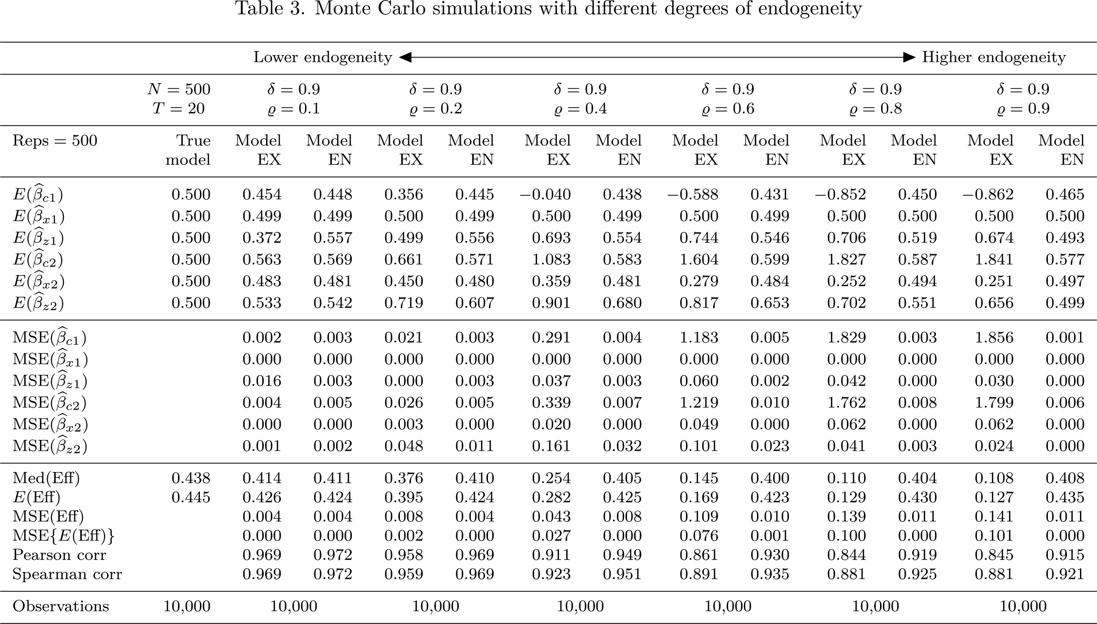
Finally, table 3 reports the simulation results with different degrees of endogeneity, with δ set to 0.9 (strong IVs). Again, N is set to 500, and T is set to 20. This table shows that with higher endogeneity (ϱ > 0.6), model EN performs better than model EX, but as the degree of endogeneity decreases, the performance of model EX becomes somewhat equivalent to that of model EN. Also, tables 2 and 3 jointly imply that if the degree of endogeneity is very low, then it may be better to use model EX, because model EN’s performance requires finding strong IVs.

Table 1.

Monte Carlo simulations with different sizes of data

Smaller data ↔Bigger data
	δ = 0.9ϱ = 0.9	N = 100T = 5		N = 500T = 10		N = 1000T = 10		N = 500T = 20		N = 1000T = 20		N = 5000T = 40
Reps = 500	TrueModel	Model EX	Model EN	Model EX	Model EN	Model EX	Model EN	Model EX	Model EN	Model EX	Model EN	Model EX	Model EN
$E (\hat{β_{c 1}})$	0.500	−0.186	0.494	−0.614	0.481	−0.617	0.481	−0.862	0.465	−0.862	0.465	−1.000	0.442
$E (\hat{β_{x 1}})$	0.500	0.499	0.501	0.500	0.500	0.500	0.500	0.500	0.500	0.500	0.500	0.500	0.500
$E (\hat{β_{z 1}})$	0.500	0.701	0.497	0.682	0.495	0.682	0.495	0.674	0.493	0.674	0.493	0.670	0.494
$E (\hat{β_{c 2}})$	0.500	1.237	0.527	1.639	0.553	1.643	0.556	1.841	0.577	1.842	0.578	1.945	0.606
$E (\hat{β_{x 2}})$	0.500	0.341	0.508	0.278	0.501	0.278	0.501	0.251	0.497	0.251	0.497	0.238	0.494
$E (\hat{β_{z 2}})$	0.500	0.824	0.511	0.709	0.503	0.708	0.503	0.656	0.499	0.656	0.500	0.629	0.497
$MSE (\hat{β_{c 1}})$		0.471	0.000	1.242	0.000	1.249	0.000	1.856	0.001	1.855	0.001	2.251	0.003
$MSE (\hat{β_{x 1}})$		0.000	0.000	0.000	0.000	0.000	0.000	0.000	0.000	0.000	0.000	0.000	0.000
$MSE (\hat{β_{z 1}})$		0.040	0.000	0.033	0.000	0.033	0.000	0.030	0.000	0.030	0.000	0.029	0.000
$MSE (\hat{β_{c 2}})$		0.544	0.001	1.297	0.003	1.307	0.003	1.799	0.006	1.801	0.006	2.089	0.011
$MSE (\hat{β_{x 2}})$		0.025	0.000	0.049	0.000	0.049	0.000	0.062	0.000	0.062	0.000	0.068	0.000
$MSE (\hat{β_{z 2}})$		0.105	0.000	0.044	0.000	0.043	0.000	0.024	0.000	0.024	0.000	0.017	0.000
Med(Eff)	0.438	0.220	0.424	0.139	0.415	0.139	0.415	0.108	0.408	0.108	0.408	0.093	0.399
E(Eff)	0.445	0.246	0.447	0.161	0.441	0.161	0.441	0.127	0.435	0.127	0.435	0.111	0.426
MSE(Eff)		0.048	0.025	0.112	0.019	0.097	0.016	0.141	0.011	0.133	0.011	0.156	0.008
MSE{E(Eff)}		0.037	0.002	0.076	0.000	0.076	0.000	0.101	0.000	0.101	0.000	0.114	0.001
Pearson corr		0.846	0.806	0.848	0.871	0.849	0.872	0.845	0.915	0.845	0.915	0.842	0.942
Spearman corr		0.864	0.811	0.878	0.879	0.878	0.880	0.881	0.921	0.881	0.922	0.882	0.946
Observations	N × T	500		5,000		10,000		10,000		20,000		200,000

Table 2.

Monte Carlo simulations with different strengths of IVs

Weaker IVs ↔Stronger IVs
	N = 500 T = 20	δ = 0.1 ϱ = 0.9		δ = 0.2 ϱ = 0.9		δ = 0.4 ϱ = 0.9		δ = 0.6 ϱ = 0.9		δ = 0.8 ϱ = 0.9		δ = 0.9 ϱ = 0.9
Reps = 500	True Model	Model EX	Model EN	Model EX	Model EN	Model EX	Model EN	Model EX	Model EN	Model EX	Model EN	Model EX	Model EN
$E (\hat{β_{c 1}})$	0.500	−0.315	0.504	−0.364	0.518	−0.433	0.500	−0.581	0.497	−0.796	0.471	−0.862	0.465
$E (\hat{β_{x 1}})$	0.500	0.500	0.505	0.501	0.504	0.500	0.500	0.500	0.499	0.500	0.500	0.500	0.500
$E (\hat{β_{z 1}})$	0.500	0.525	3.940	0.580	3.439	0.679	1.779	0.722	0.563	0.700	0.525	0.674	0.493
$E (\hat{β_{c 2}})$	0.500	1.386	0.546	1.429	0.539	1.495	0.551	1.622	0.547	1.793	0.573	1.841	0.577
$E (\hat{β_{x 2}})$	0.500	0.311	0.509	0.305	0.508	0.299	0.504	0.282	0.501	0.258	0.497	0.251	0.497
$E (\hat{β_{z 2}})$	0.500	0.708	0.053	0.716	0.116	0.703	0.267	0.682	0.386	0.663	0.485	0.656	0.499
$MSE (\hat{β_{c 1}})$		0.665	0.000	0.746	0.000	0.870	0.000	1.169	0.000	1.680	0.001	1.856	0.001
$MSE (\hat{β_{x 1}})$		0.000	0.000	0.000	0.000	0.000	0.000	0.000	0.000	0.000	0.000	0.000	0.000
$MSE (\hat{β_{z 1}})$		0.001	11.831	0.006	8.636	0.032	1.635	0.049	0.004	0.040	0.001	0.030	0.000
$MSE (\hat{β_{c 2}})$		0.786	0.002	0.863	0.002	0.990	0.003	1.259	0.002	1.671	0.005	1.799	0.006
$MSE (\hat{β_{x 2}})$		0.036	0.000	0.038	0.000	0.040	0.000	0.048	0.000	0.058	0.000	0.062	0.000
$MSE (\hat{β_{z 2}})$		0.043	0.200	0.047	0.148	0.041	0.054	0.033	0.013	0.027	0.000	0.024	0.000
Med(Eff)	0.438	0.186	0.425	0.178	0.426	0.167	0.421	0.143	0.420	0.115	0.410	0.108	0.408
E(Eff)	0.445	0.212	0.445	0.202	0.447	0.189	0.446	0.164	0.446	0.134	0.437	0.127	0.435
MSE(Eff)		0.079	0.014	0.087	0.013	0.091	0.014	0.112	0.013	0.135	0.012	0.141	0.011
MSE{E(Eff)}		0.055	0.000	0.059	0.000	0.066	0.000	0.079	0.000	0.096	0.000	0.101	0.000
Pearson corr		0.814	0.897	0.820	0.896	0.842	0.900	0.851	0.905	0.847	0.912	0.845	0.915
Spearman corr		0.832	0.900	0.840	0.899	0.863	0.905	0.876	0.910	0.880	0.919	0.881	0.921
Observations	10,000	10,000		10,000		10,000		10,000		10,000		10,000

Table 3.

Monte Carlo simulations with different degrees of endogeneity

Lower endogeneity ↔Higher endogeneity
	N = 500 T = 20	δ = 0.9 ϱ = 0.1		δ = 0.9 ϱ = 0.2		δ = 0.9 ϱ = 0.4		δ = 0.9 ϱ = 0.6		δ = 0.9 ϱ = 0.8		δ = 0.9 ϱ = 0.9
Reps = 500	True Model	Model EX	Model EN	Model EX	Model EN	Model EX	Model EN	Model EX	Model EN	Model EX	Model EN	Model EX	Model EN
$E (\hat{β_{c 1}})$	0.500	0.454	0.448	0.356	0.445	−0.040	0.438	−0.588	0.431	−0.852	0.450	−0.862	0.465
$E (\hat{β_{x 1}})$	0.500	0.499	0.499	0.500	0.499	0.500	0.499	0.500	0.499	0.500	0.500	0.500	0.500
$E (\hat{β_{z 1}})$	0.500	0.372	0.557	0.499	0.556	0.693	0.554	0.744	0.546	0.706	0.519	0.674	0.493
$E (\hat{β_{c 2}})$	0.500	0.563	0.569	0.661	0.571	1.083	0.583	1.604	0.599	1.827	0.587	1.841	0.577
$E (\hat{β_{x 2}})$	0.500	0.483	0.481	0.450	0.480	0.359	0.481	0.279	0.484	0.252	0.494	0.251	0.497
$E (\hat{β_{z 2}})$	0.500	0.533	0.542	0.719	0.607	0.901	0.680	0.817	0.653	0.702	0.551	0.656	0.499
$MSE (\hat{β_{c 1}})$		0.002	0.003	0.021	0.003	0.291	0.004	1.183	0.005	1.829	0.003	1.856	0.001
$MSE (\hat{β_{x 1}})$		0.000	0.000	0.000	0.000	0.000	0.000	0.000	0.000	0.000	0.000	0.000	0.000
$MSE (\hat{β_{z 1}})$		0.016	0.003	0.000	0.003	0.037	0.003	0.060	0.002	0.042	0.000	0.030	0.000
$MSE (\hat{β_{c 2}})$		0.004	0.005	0.026	0.005	0.339	0.007	1.219	0.010	1.762	0.008	1.799	0.006
$MSE (\hat{β_{x 2}})$		0.000	0.000	0.003	0.000	0.020	0.000	0.049	0.000	0.062	0.000	0.062	0.000
$MSE (\hat{β_{z 2}})$		0.001	0.002	0.048	0.011	0.161	0.032	0.101	0.023	0.041	0.003	0.024	0.000
Med(Eff)	0.438	0.414	0.411	0.376	0.410	0.254	0.405	0.145	0.400	0.110	0.404	0.108	0.408
E(Eff)	0.445	0.426	0.424	0.395	0.424	0.282	0.425	0.169	0.423	0.129	0.430	0.127	0.435
MSE(Eff)		0.004	0.004	0.008	0.004	0.043	0.008	0.109	0.010	0.139	0.011	0.141	0.011
MSE{E(Eff)}		0.000	0.000	0.002	0.000	0.027	0.000	0.076	0.001	0.100	0.000	0.101	0.000
Pearson corr		0.969	0.972	0.958	0.969	0.911	0.949	0.861	0.930	0.844	0.919	0.845	0.915
Spearman corr		0.969	0.972	0.959	0.969	0.923	0.951	0.891	0.935	0.881	0.925	0.881	0.921
Observations	10,000	10,000		10,000		10,000		10,000		10,000		10,000

5 Empirical examples

In this section, I present three different examples to illustrate the usage of xtsfkk. In all examples, eta endogeneity test results show that there are endogeneity problems in the models, and the results that correct for the endogeneity are substantially different than the results that ignore endogeneity.

5.1 Panel stochastic production frontier model with endogeneity

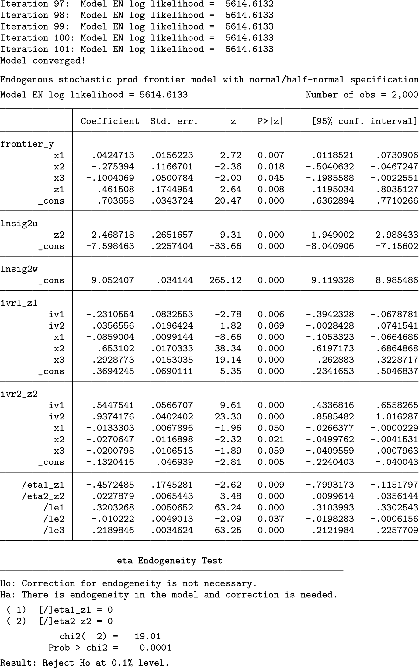
The first example analyzes a randomly generated longitudinal dataset in a production setting. This dataset is for illustrative purposes and does not represent a particular industry. The unbalanced panel dataset has a total of 2,000 observations of 140 firms between 1991 and 2015. Production (y) is modeled by some frontier variables (x1, x2, x3, and z1), and inefficiency is modeled by a different variable (z2). Two variables, one in the frontier and one in the inefficiency function (z1 and z2), are assumed to be endogenous, and two IVs (iv1 and iv2) are used to handle the endogeneity. To display the model fully, the header option is added to the command line.

Raw estimation results are presented in the table; eta terms for z1 and z2 are both statistically significant in the table. Also, because the test option was specified, eta endogeneity test results are presented, showing that the null hypothesis is rejected at the 0.1% level and correction for endogeneity is needed. Looking at the coefficients of the endogenous variables, z1 and z2 are both positive and statistically significant. If the compare option had been specified, the results from the exogenous comparison model would show that the coefficients of z1 and z2 are substantially smaller than they are in the displayed model corrected for endogeneity.

Because the efficiency() option was specified in the command line, technical efficiency scores are saved as a variable and this variable’s summary statistics are presented. In this model, mean technical efficiency is 0.9719 and median technical efficiency is 0.9722. If the compare option had been specified, the efficiency() option would also save the efficiency scores from the model that ignores endogeneity. A comparison of technical efficiencies from these two models would indicate that some producers are not as efficient in production as they would appear in a standard frontier model that ignores endogeneity.

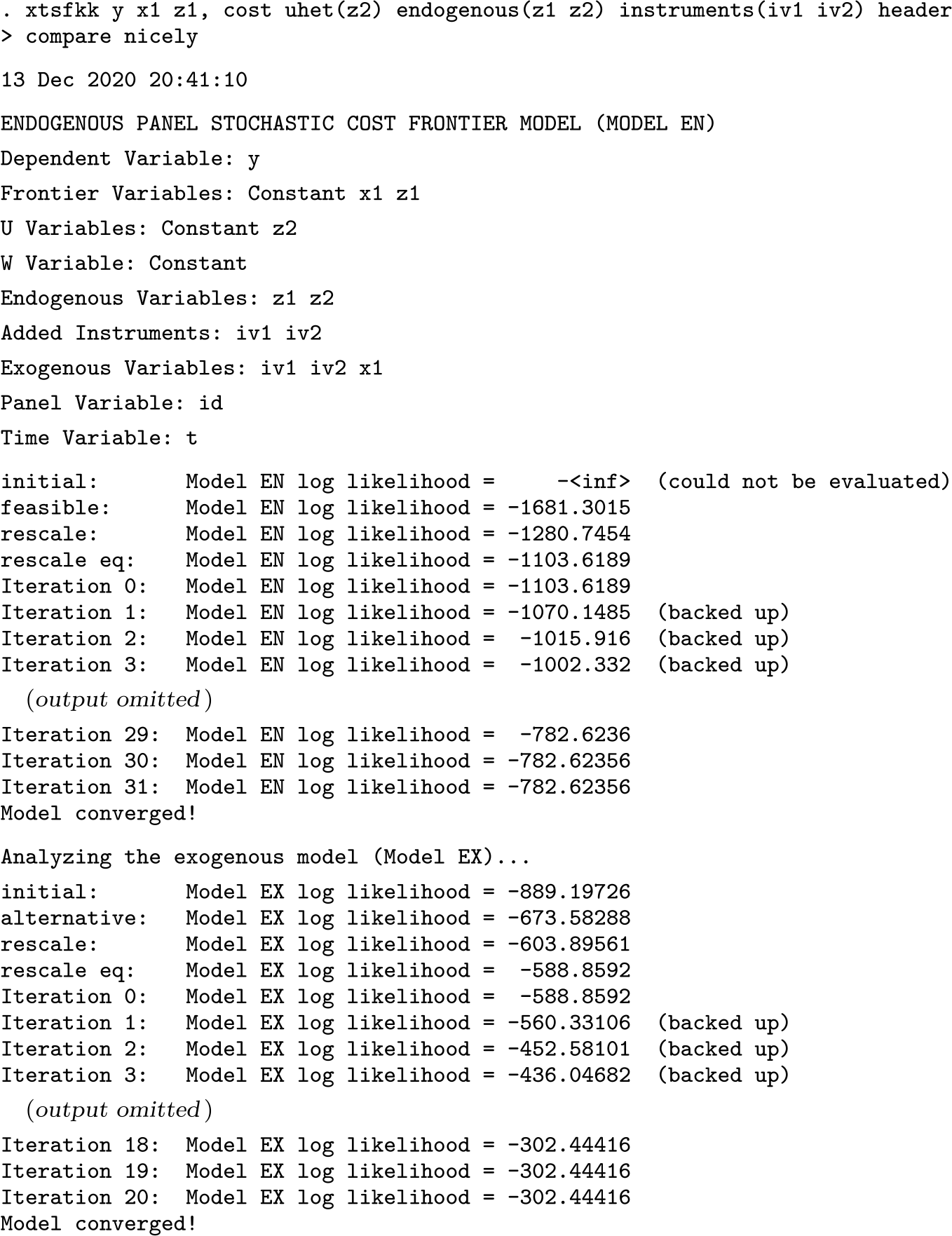
5.2 Panel stochastic cost frontier model with endogeneity

In this example, the longitudinal data include 85 individuals and a total of 300 observations between 2011 and 2015. This unbalanced dataset is for illustrative purposes and does not characterize a certain sector. The cost (y) is modeled as a function of two frontier variables (x1 and z1), and cost inefficiency is modeled as a function of a variable (z2). Two IVs (iv1 and iv2) are used to handle the potential endogeneity of two variables (z1 and z2) in the model. The header option displays the model fully.

The output table above presents the estimation results. Because the compare and nicely options were specified, there are two columns of results: model EX is the model that ignores endogeneity, and model EN is the model that handles endogeneity. Individual eta terms for z1 and z2 are both statistically significant at the 0.1% level, and the eta endogeneity test result rejects the null hypothesis at the 0.1% level, which indicates that a correction for endogeneity in the model is necessary.

Statistical significance and magnitudes of coefficients are different in model EX and model EN. The coefficients of z1 and z2 in model EX are positive and statistically significant. In model EN, these coefficients are significant and positive but smaller. Moreover, mean cost efficiency in model EX is 0.3625, while in model EN, the same statistic is 0.4838. This tells us that individuals in the model with endogeneity are more cost efficient than they would be in the model that overlooks endogeneity.

5.3 Example from the U.S. banking sector

In this last example, we examine a panel stochastic production frontier model with a real dataset that comes from the U.S. banking sector. The main panel data are from the Federal Financial Institutions Examination Council Central Data Repository. This main panel dataset consists of 19,304 year-end observations of 4,408 U.S. banks from 2010 to 2016. We follow the model in Berger et al. (2017) and, for simplicity, design a simpler loan production model where the dependent variable is the natural logarithm of total small loans (loans). Production frontier variables include natural logarithms of core deposits (cdep), other hot money (hotm), and gross total assets (gta). Also, the frontier function includes bank return on equity (roe) and a dummy variable (big) that is equal to 1 if the gross total assets of the bank is greater than $1 billion. Technical inefficiency is modeled with a Herfindahl–Hirschman index (hhi) of market concentration ranging between 0 and 1, with 1 indicating a monopoly setting. We control for the endogeneity of loans and hhi by using the leading political party’s voter representation percentage in a county.¹

We specify the compare, nicely, header, save(), and load() options in this example. Model EX, which does not handle endogeneity, is comparable with a standard xtfrontier command estimation. The coefficient of hhi is expected to be negative. Looking at the results, we see that the eta term of hhi is significant at the 0.1% level, and the eta endogeneity test result tells us that correction for endogeneity is necessary. As shown in the output table below, the coefficient of hhi is negative and significant in model EX, but in model EN, the coefficient is substantially smaller (bigger negative impact) and significant.

6 Conclusion

In this article, I offered a new command called xtsfkk to fit endogenous stochastic panel frontier models, presented by Karakaplan and Kutlu (2017a). xtsfkk can control for the endogenous variables in both the frontier and the inefficiency term. With some Monte Carlo simulations and examples, I showed that xtsfkk outperforms the standard panel frontier estimation methods that ignore endogeneity. Moreover, xtsfkk comes with various options that can be useful in panel research settings.

8 Programs and supplemental materials

Supplemental Material, sj-zip-1-stj-10.1177_1536867X221124539 - Panel stochastic frontier models with endogeneity

Supplemental Material, sj-zip-1-stj-10.1177_1536867X221124539 for Panel stochastic frontier models with endogeneity by Mustafa U. Karakaplan in The Stata Journal

Footnotes

Notes

7 Acknowledgments

I thank Levent Kutlu, Hung-Jen Wang, Isabel Canette, Joerg Luedicke, Ben Jann, Jan Ditzen, Myk Milligan, Kit Baum, and an anonymous referee for their great support. I also acknowledge that the Research Computing program under the Division of Information Technology at the University of South Carolina contributed to the results in this research by providing High Performance Computing resources and expertise.

8 Programs and supplemental materials

To install a snapshot of the corresponding software files as they existed at the time of publication of this article, type

References

Aigner

D. J.

Lovell

C. A. K.

Schmidt

1977. Formulation and estimation of stochastic frontier production function models. Journal of Econometrics 6: 21–37. https://doi.org/10.1016/0304-4076(77)90052-5.

Amadou

D. I

. 2012. frontierhtail: Stata module to estimate stochastic production frontier models for heavy tail data. Statistical Software Components S457398, Department of Economics, Boston College. https://ideas.repec.org/c/boc/bocode/s457398.html.

Baum

C. F.

Gould

2004. matin4-matout4: Stata module to import and export matrices. Statistical Software Components S445101, Department of Economics, Boston College. https://ideas.repec.org/c/boc/bocode/s445101.html.

Belotti

Daidone

Ilardi

Atella

2013. Stochastic frontier analysis using Stata. Stata Journal 13: 719–758. https://doi.org/10.1177/1536867X1301300404.

Berger

A. N.

Black

L. K.

Bouwman

C. H. S.

Dlugosz

2017. Bank loan supply responses to Federal Reserve emergency liquidity facilities. Journal of Financial Intermediation 32: 1–15. https://doi.org/10.1016/j.jfi.2017.02.002.

Ditzen

. 2019. simulate2: Stata module enhancing and parallelising simulate. Statistical Software Components S458703, Department of Economics, Boston College. https://ideas.repec.org/c/boc/bocode/s458703.html.

Fé

Hofler

2013. Count data stochastic frontier models, with an application to the patents—R&D relationship. Journal of Productivity Analysis 39: 271–284. https://doi.org/10.1007/s11123-012-0286-y.

Fé

Hofler

2020. sfcount: Command for count-data stochastic frontiers and underreported and overreported counts. Stata Journal 20: 532–547. https://doi.org/10.1177/1536867X20953566.

Germeshausen

Panke

Wetzel

2020. Firm characteristics and the ability to exercise market power: Empirical evidence from the iron ore market. Empirical Economics 58: 2223–2247. https://doi.org/10.1007/s00181-018-1610-9.

10.

Gould

Pitblado

Poi

2010. Maximum Likelihood Estimation with Stata. 4th ed. College Station, TX: Stata Press.

11.

Gupta

A. K.

Nguyen

2010. Stochastic frontier analysis with fat-tailed error models. Far East Journal of Theoretical Statistics 31: 77–95.

12.

Jann

2005. Making regression tables from stored estimates. Stata Journal 5: 288–308. https://doi.org/10.1177/1536867X0500500302.

13.

Karakaplan

M. U.

2017. Fitting endogenous stochastic frontier models in Stata. Stata Journal 17: 39–55. https://doi.org/10.1177/1536867X1701700103.

14.

Karakaplan

M. U.

Kutlu

2017a. Handling endogeneity in stochastic frontier analysis. Economics Bulletin 37: 889–901.

15.

Karakaplan

M. U.

Kutlu

2017b. Endogeneity in panel stochastic frontier models: An application to the Japanese cotton spinning industry. Applied Economics 49: 5935–5939. https://doi.org/10.1080/00036846.2017.1363861.

16.

Karakaplan

M. U.

Kutlu

2019. School district consolidation policies: Endogenous cost inefficiency and saving reversals. Empirical Economics 56: 1729–1768. https://doi.org/10.1007/s00181-017-1398-z

17.

Kumbhakar

S. C.

Lovell

C. A. K.

2000. Stochastic Frontier Analysis. Cambridge: Cambridge University Press.

18.

Kumbhakar

S. C.

Wang

H.-J.

Horncastle

A. P.

2015. A Practitioner’s Guide to Stochastic Frontier Analysis Using Stata. Cambridge: Cambridge University Press.

19.

Kutlu

. 2010. Battese–Coelli estimator with endogenous regressors. Economics Letters 109: 79–81. https://doi.org/10.1016/j.econlet.2010.08.008.

20.

Levinsohn

Petrin

2003. Estimating production functions using inputs to control for unobservables. Review of Economic Studies 70: 317–341. https://doi.org/10.1111/1467-937X.00246.

21.

Meeusen

van den Broeck

1977. Efficiency estimation from Cobb–Douglas production functions with composed error. International Economic Review 18: 435–444. https://doi.org/10.2307/2525757.

22.

Olley

G. S.

Pakes

1996. The dynamics of productivity in the telecommunications equipment industry. Econometrica 64: 1263–1297. https://doi.org/10.2307/2171831.

23.

Petrin

Poi

B. P.

Levinsohn

2004. Production function estimation in Stata using inputs to control for unobservables. Stata Journal 4: 113–123. https://doi.org/10.1177/1536867X0400400202.

24.

Wang

H.-J

. 1999. gentrun: Stata module to generate truncated normal variate. Statistical Software Components S400501, Department of Economics, Boston College. https://ideas.repec.org/c/boc/bocode/s400501.html.

25.

X.-L.

Chen

H. H.

2018. Examining the efficiency of biomass energy: Evidence from the Chinese recycling industry. Energy Policy 119: 77–86. https://doi.org/10.1016/j.enpol.2018.04.020.

26.

Yasar

Raciborski

Poi

2008. Production function estimation in Stata using the Olley and Pakes method. Stata Journal 8: 221–231. https://doi.org/10.1177/1536867X0800800204.