
Abstract
In this article, we describe the package
Keywords
1 Introduction
Datasets in which lower-level units are nested within higher-level units are frequent in many disciplines. Prime examples in the social sciences are data in which students are clustered within schools, or respondents of international surveys are clustered within countries. In medical research, we find cluster randomized trials, in which, for example, individuals are assigned to receive a control or intervention condition within health clinics or villages (Hayes and Moulton 2017). Observational studies of animals clustered by habitats or cells in organisms are further examples. In linguistics, words are nested within corpora. Further examples from various disciplines could be easily listed.
Data containing several levels are typically termed “hierarchical data” or “multilevel data”. In this article, we focus exclusively on the two-level case, which is arguably the most common. In what follows, we use the term “microlevel” to refer to the first (lowest) level and “macrolevel” to refer to the second level within which first-level units are nested. Correspondingly, microlevel covariates are those that differ across first-level units, and macrolevel covariates are those that vary across second-level units and are common to clusters of first-level units.
The analysis of hierarchical data poses challenges, primarily for the estimation of standard errors but also for the estimation of the effects of macrolevel covariates on a microlevel outcome or of interactions between microlevel and macrolevel covariates (cross-level interactions [CLIs]). The two-step approach discussed here is primarily targeted for studying such higher-level effects and particularly CLIs.
In general, four approaches to modeling hierarchical data can be distinguished (Bryan and Jenkins 2016a, 4–5): regression analysis with cluster–robust standard errors, fixed macrolevel intercept terms, mixed models with macrolevel random effects, and separate analyses on the microlevel for each unit of the macrolevel with subsequent analysis of their results. This article focuses on the last approach, which is commonly referred to as the two-step approach. The two-step approach can be used for hierarchical data with two levels and is particularly useful for data with many observations at the microlevel and a rather limited number of observations at the macrolevel; see section 2 for merits of the two-step approach.
The implementation of the two-step approach in Stata is very simple, as can be shown by the following example using data from a cross-nationally comparative European survey in which individual respondents are nested within countries (discussed further in section 4). After loading the data,

we run a regression for each country (the macrolevel units) separately and write the regression coefficients to the active data frame. In our example, we regress the respondents’ general life satisfaction on household income, sex, and age:

In the second step, selected regression coefficients of these regression models are further analyzed. The standard case is to study their associations with macrolevel covariates. Continuing with our example, we merge a file containing macrolevel variables to the estimated country-level regression coefficients and study how the effect of household income on life satisfaction covaries with a country’s gross domestic product (that is, the CLI of household income and gross domestic product [GDP]):

Typical extensions to this approach involve more formal refinements of the second step’s regression models, exploratory data analysis (EDA) techniques concerning both steps’ analyses, meaningful graphical displays of the results, or the diagnosis of the assumptions of other approaches to study hierarchical data. This article presents the new command
2 The two-step approach in context
Applying the two-step approach to hierarchical data serves various intentions. Setting up regression models—known as hierarchical or multilevel models—is probably the most important objective researchers have in mind when facing hierarchical data. Accordingly, section 2.1 discusses to what extent the two-step approach can offer an alternative to other approaches that are commonly applied to model hierarchical data. However, the two-step approach can also be used to facilitate refinement of hierarchical models by providing tools for further data exploration, visual representation of results, and conducting diagnostic checks. These applications of the two-step approach are discussed in section 2.2. Section 2.3 documents the methods and formulas for
2.1 Modeling hierarchical data
The defining characteristic of hierarchical data is its nested data structure. In the following, we consider the case where microlevel units i are nested within macrolevel units j; that is, we consider a two-level structure. Given this data structure, a typical (linear) model is


where yij is a continuous outcome variable and
By inserting (2) into (1), we can also express this model as

This model is sometimes called a direct context effect (DCE) model (Heisig, Schaeffer, and Giesecke 2017) because it directly relates macrolevel characteristics to levels of yij.
The DCE model allows yij to depend on


where now
Again, the multiple-equation representation above can be converted into a singleequation representation by inserting (4) and (5) into (3):

Such models are commonly known as CLI models, because the effect of at least one microlevel variable is assumed to depend on the levels of at least one macrolevel variable.
Bryan and Jenkins (2016a, 4–5) differentiate between four general approaches to estimating the parameters of interest in DCE and CLI models. In all of these four approaches, the unmeasured effects u0
j
, ukj, and ϵij are assumed to be uncorrelated with both Pooling the data
1
using cluster–robust standard errors. This approach allows estimation of both DCE and CLI models. To account for the clustering of the data, this approach is implemented in Stata with the option Pooling the data and including a set of dummy variables for the macrolevel units. By directly allowing fixed-effects for all macrolevel units, this approach does not allow the inclusion of macrolevel characteristics Pooling the data and specifying random effects. This approach permits fitting both DCE and CLI models; that is, some of or all the Fitting separate models for each unit j of the macrolevel. When you stratify the analysis on the units of the macrolevel, all
Each approach has its pros and cons; see Bryan and Jenkins (2016b, 5–10) for a lucid comparison. In brief, the random-effects approach—if specified correctly—is more efficient than the two-step approach, and both approaches show better statistical performance when compared with the cluster–robust and the fixed-effects approach (for a simulation study, see Heisig, Schaeffer, and Giesecke [2017]). However, the twostep approach is a valuable and easy-to-implement alternative to the random-effects approach, in particular if the number of microlevel observations within each macrolevel unit is large and the number of macrolevel units is small. 4 In the following, we want to highlight three arguments for applying the two-step approach for analyzing hierarchical data.
First, the two-step approach brings the scarcity of data points at the macrolevel to the attention of the researcher, which may motivate caution regarding influential data points. Consequently, the two-step approach also highlights to the researcher that there is a practical limit on the number of macrolevel variables that can be included in the second-step regression (Bryan and Jenkins 2016b, 10).
Second, the random-effects approach relies on several distributional assumptions to estimate the
A more formal statistical problem is that the standard errors of the macrolevel coefficients
For such problems, the two-step approach could be used as a direct alternative to the one-step approach. However, the two-step approach has its own challenges. The model estimated at the second step is heteroskedastic because sampling errors of the parameters estimated at the microlevel are likely to vary between the macrolevel units. It has been pointed out, though, that with many observations at the microlevel, the sampling errors should be sufficiently small so that the second step can done by ordinary least squares (OLS) (Donald and Lang 2007; Wooldridge 2010, 891–892). Moreover, Hanushek (1974), Borjas and Sueyoshi (1994), Lewis and Linzer (2005), and Donald and Lang (2007) provide weighting matrices for feasible generalized least squares (FGLS). According to Bryan and Jenkins (2016b, n. 4), those FGLS estimates are consistent only (and distributed normally) for large numbers of units at the macrolevel, leading Bryan and Jenkins (2016b) to prefer the OLS over FGLS for the second step.
2.2 Descriptive hierarchical data analysis
While statistical inference about
Three specific—but strongly overlapping—descriptive purposes come to our mind: EDA. The two-step approach gives direct access to the first-step’s model parameters. This dataset can be studied with any of the many techniques for EDA; see, for example, Bowers and Drake (2005). Particularly, scatterplots between the coefficients estimated in the microlevel models and macrolevel variables may inspire further hypotheses. Descriptive graphs. The graphical techniques used for EDA can also be used as a graphical device for presenting the results. In addition, a simple graph of the coefficients estimated in the microlevel models for each macrolevel unit may be used. This graph can be also used to communicate estimates for Diagnostics. Because the two-step approach does not pose any assumptions on the distribution of the parameters in the microlevel models, the actual distribution of those parameters can be used to check the validity of the assumptions of the one-step approach.
The command
Before describing the actual command, we document the formulas for
2.3 Methods and formulas
Closely following Lewis and Linzer (2005), this subsection documents the formulas for all methods implemented in

Using the two-step approach, we first estimate (7) separately for each macrolevel unit j, yielding J estimates for each of the

If βkj is modeled to depend on
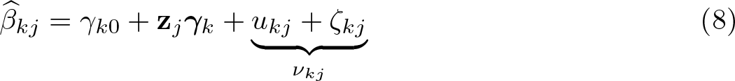
The error term in (8) is a composite of the sampling error ζkj and the error of the macrolevel regression. In line with (5), we denote the latter with ukj and the joint error term with νkj.
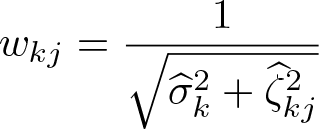
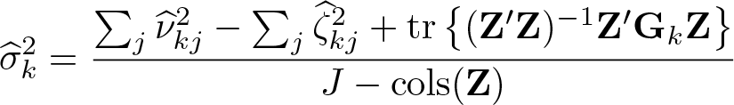
The sampling variance of

where

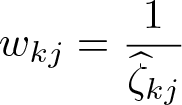
where the weights wkj are defined as
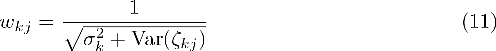
Equation (11) demonstrates that those macrolevel units j with lower (higher) sampling error with respect to estimating βkj in the first step get higher (lower) weights in the second-step estimation.
Using (9), the proportion of the total error variance in the macrolevel model arising from the sampling variance in the microlevel models can be defined as
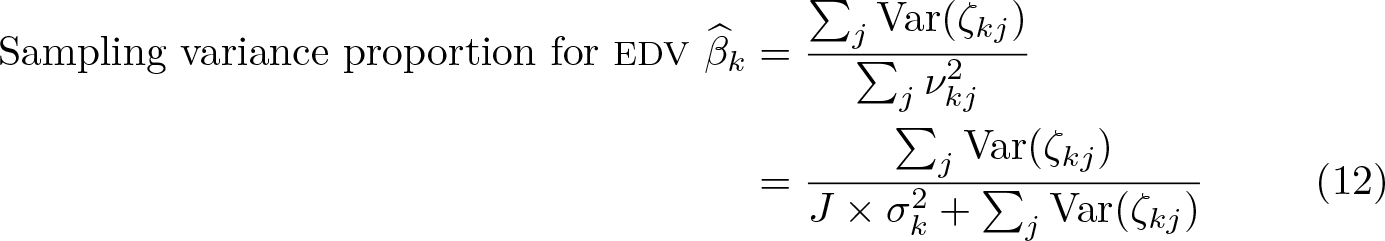
The sampling variance proportion is displayed below the table of coefficients in the corresponding output of
In practice,
The simplest case sets all weights to be constant; that is,
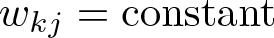
which basically assumes that ζkj does not vary between macrolevel units so that Var(νkj) is assumed to be constant as well. Setting all wkj to a constant term results in (5) being estimated by OLS. This yields efficient estimates and consistent standard errors of the
Saxonhouse (1976) proposes setting the weights to
where
Hanushek (1974) proposes to set the weights to
with
with

and
Hanushek’s method assumes that the microlevel estimates of
Lewis and Linzer (2005, 353) derive another set of weights for the case that the number of observations used for microlevel regressions is known, but the standard errors of the
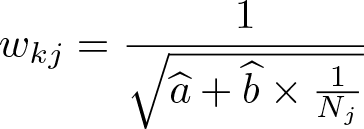
with
Simulations for more specific characteristics of the estimators under various conditions can be found in Lewis and Linzer (2005), Donald and Lang (2007), Bryan and Jenkins (2016a), Heisig, Schaeffer, and Giesecke (2017), and Heisig and Schaeffer (2019).
3 The command twostep
3.1 General syntax
The general syntax of
In the following, we discuss commonalities of the syntax for each of these three sections. We then continue by describing the microlevel commands as well as the macrolevel commands.
3.1.1 Declaration
The hierarchical structure of the data is declared using the prefix command
macroid refers to a varlist that identifies the macrolevel units in the combined micro– macro-level data. Factor-variable notation is not allowed.
The option
3.1.2 Microlevel command
The microlevel_command can be either a Stata estimation command or one of the special-purpose commands
Users may specify any estimation command such as
The special-purpose command
3.1.3 Macrolevel command
The macrolevel_command may be one of the following special-purpose commands, which we order here according to the typical uses proposed in section 2:
Estimating CLIs
EDA
macrodepvar macroindepvars [if] [in] [
(The last syntax does not contain the name of a macrolevel command; see section 3.3.)
Descriptive graphs
Diagnostics
cmd macrodepvar macroindepvars [if] [in] [
Allow more customized analyses
All the macrolevel commands have a common syntax. For all the commands, macrodepvar refers to a coefficient or summary statistic of the first step’s microlevel model. The coefficients are referred to by adding
macroindepvars refer to a varlist of macrolevel variables. Factor-variable notation is allowed; see [U]
filename refers to a dataset containing the macrolevel variables except for the statistics estimated at the microlevel. In this dataset, the macroid specified in the declaration of
3.2 Specific remarks on macrolevel commands
3.2.1 edv
The macrolevel command
It fits the microlevel models separately for each macrolevel unit.
It creates a variable for weighting the macrolevel model; see section 2.3 for the calculation of the weighting variable.
It runs a linear regression of the selected coefficient on the specified macrolevel variables, weighted by the created weight variable.
The command shares the syntax of all macrolevel commands but allows the following specific options:
regress_options all options allowed for [R]
3.2.2 avplot
The macrolevel command
It fits the microlevel models separately for each macrolevel unit.
It runs a linear regression of depvar on varlist; by default, the regression is weighted according to the default setting of the command
It creates an added-variable plot with an overlaid regression line, whereby the marker symbols are drawn in a size proportional to the weights of the EDV model. In addition, all marker symbols are labeled in a lighter shade of gray with the value labels or values of macroid.
In the special case of a macrolevel model with just one independent variable, the added-variable plot is identical to a bivariate scatterplot of the mean-centered outcome variable against the mean-centered independent variable.
The command shares the syntax of all macrolevel commands but allows the following specific options:
regress_options refer to the options
twoway_options are options allowed for [R]
3.2.3 cprplot
The macrolevel command
It fits the microlevel models separately for each macrolevel unit.
It runs a linear regression of depvar on varlist; by default, the regression is weighted according to the default setting of the macrolevel command
It draws a component-plus-residual plot with an overlaid regression line and LOWESS, whereby the marker symbols are drawn in a size proportional to the weights. In addition, all marker symbols are labeled with the value labels or values of macroid.
In the special case of a macrolevel model with just one independent variable, the component-plus-residual plot is identical to a bivariate scatterplot of the mean-centered outcome variable against the independent variable.
The command shares the syntax of all macrolevel commands. It allows the same options as the macrolevel command
3.2.4 regby
The macrolevel command
It fits the microlevel models separately for each macrolevel unit.
It classifies the macrolevel observations into groups defined by macrolevel variables specified with macroindepvars. By default, these groups are created by crossclassifying dichotomized versions of those macrolevel variables.
It creates plots of the coefficients estimated in the first step and selected by macrodepvar. More specifically, it plots regression lines for each macrolevel observation and groups these plots according to the (cross-classified) groups defined by macroindepvars. The plotted regression lines are defined by a slope that corresponds to the value of the coefficient estimated in the first step and are plotted over the range of the underlying microlevel variable.
To ease the comparison between groups, we have each of the subgraphs also show lines for all macrolevel observations in a lighter shade of gray.
The command shares the syntax of all macrolevel commands and allows the following specific options:
twoway_options are options allowed for [G-2]
3.2.5 dot
The macrolevel command
It fits the microlevel models separately for each macrolevel unit.
It sorts the estimated coefficients or summary statistics according to the predefined or a user-specified criterion.
It draws a horizontally labeled dot chart of the coefficients or summary statistics. If coefficients are displayed, the dots are amended by confidence intervals.
The command shares the syntax of all macrolevel commands and allows the following specific options:
twoway_options are options allowed for [G-2]
3.2.6 cmd
Besides the more specific commands for the second step,
While this feature may be used as a kind of fallback mode for analyses not implemented directly into
3.2.7 mk2nd
The macrolevel command
The definitions of the terms are the same as for all the other macrolevel commands. The major difference is that a user can specify
We stress that the EDV model can be fit in a dataset created by the macrolevel command
Finally, the option
3.3 The special-purpose microlevel commands
In the standard case,
depvar and varlist define the dependent and independent variables of a linear regression at the microlevel. Note that using
It separately estimates a linear regression of the specified dependent variable on the specified independent variables for each macrolevel unit.
It draws a component-plus-residual plot of a selected coefficient for each of the microlevel regressions and combines them into one single graph. By default, the various subgraphs are ordered according to the size of the selected coefficient.
It separately estimates a linear regression of the specified dependent variable on the specified independent variables for each macrolevel unit.
It calculates the DFBETAs of a selected coefficient for each of the fitted microlevel regression models.
It draws the box plots of the DFBETAs over the categories of each macrolevel unit.
As mentioned above, in the case of using the special-purpose microlevel commands
Despite this difference, the specific meanings of terms remain the same as for all the other macrolevel commands. macrodepvar is used to select the independent variable for which the microlevel component-plus-residual plots and the box plots of the DFBETAs are drawn. macroindepvars specifies the order of the subgraphs and boxes and the options that are used to further control the appearance of the graphs. All options available for the macrolevel command
4 Examples
All examples in this section rely on fabricated data mimicking the European Quality of Life Survey 2003 (see European Foundation for the Improvement of Living and Working Conditions, Wissenschaftszentrum Berlin fuer Sozialforschung [2006])—a crossnationally comparative survey carried out in 28 European countries.

We wish to study the effect of household income (
4.1 Estimating CLIs
The two-step approach may be used as an alternative to the one-step approach to estimate the coefficients of CLIs. This is particularly useful if the assumptions of the various one-step approaches cannot be satisfied or if the parameters of the correct model of the one-step approach cannot be estimated because of issues of convergence. In the following, we provide Stata commands for fitting the CLI model with each of the four approaches discussed by Bryan and Jenkins (2016b).
A common strategy to estimate CLI would be to use one of the one-step approaches discussed in section 2. For sake of brevity, the following presents the Stata commands for each of the three one-step approaches without showing the output, but see table 1 for a comparison of the key findings from all four approaches. For simplicity, and because it is not unusual in the field of life-satisfaction research (for example, Hagerty and Veenhoven [2003] and Radcliff [2013]), we also rely on linear regression instead of using ordered logit or ordered probit models.
An example of the CLI model on the pooled data with cluster–robust standard errors is
One of many ways to calculate the model assuming fixed country effects is to use
Another possibility is to revert to
As theoretically expected, all models produce a statistically significant negative coefficient for the interaction term. The two-step analogue to estimate the corresponding CLI is the following:
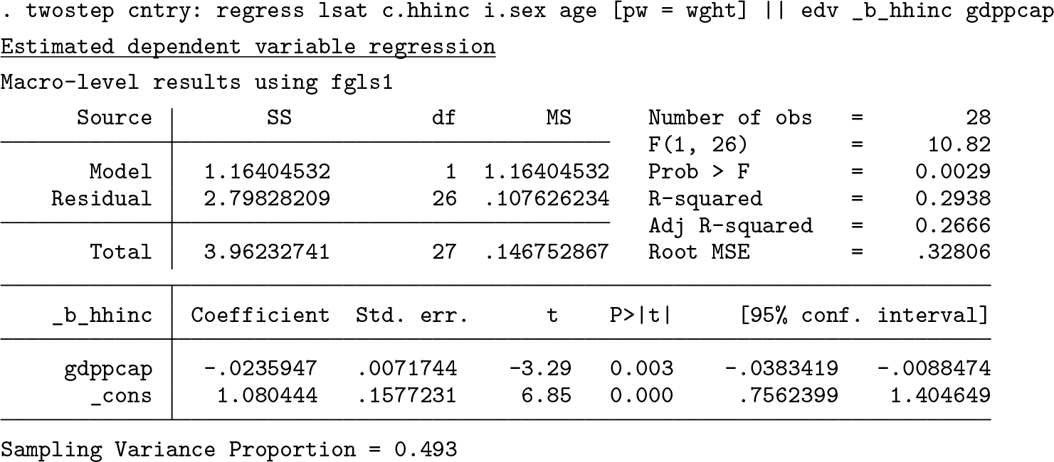
In this output, the coefficient for
Estimated CLI from the four approaches
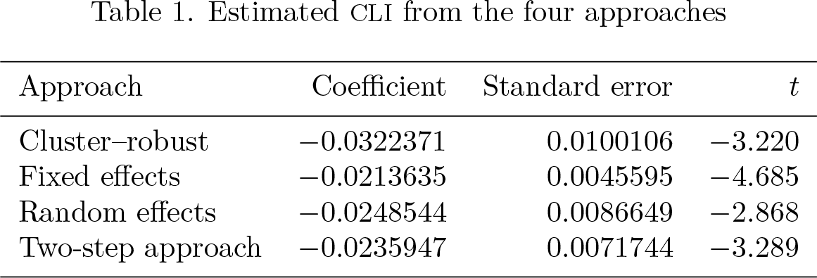
Note that separate models must be run if one is interested in the CLIs with other microlevel variables. However, one can estimate the CLI of one microlevel variable with several macrolevel variables in one model. To illustrate the flexibility of
4.2 EDA
The two-step approach is very useful for EDA. The two variants of the component-plusresidual plots may be used to point to nonlinear associations in both the microlevel models (
We stress that there is a large overlap between the kind of EDA presented here and the descriptive graphs and regression diagnostics presented in the next sections. More specifically, all the examples in this section can also be seen as regression diagnostics and as powerful devices for presenting the results. However, in the context of EDA, we consider the graphs a tool for exploration only, not meant to be presented to a larger audience. Thus, we primarily present the graphs here in their default settings. To use them for presentation, we suggest to use options similar to those shown in one of the examples of section 4.3.
4.2.1 Microlevel component-plus-residual plot
Building on our running example, we use the following command to create a componentplus-residual plot for the regressor

Component-plus-residual plot for the regression coefficient of household income for all countries
The purpose of figure 1 is to examine whether the linearity assumptions invoked for the microlevel models hold. To detect deviations, we should particularly search for countries in which the LOWESS lines (Cleveland 1979) deviate strongly from the within regression lines in dense data regions; deviations in sparse regions maybe simply result from outliers. A close inspection of the graph suggests some suspicious deviations in countries such as Slovakia, Estonia, Hungary, and others. Such deviations indicate the need for further inspection of the data in these countries, as do the strong deviations that might be attributable to outliers. A very close inspection also reveals that the dispersion of household income in Bulgaria is very small, except for one outlier.
4.2.2 Microlevel plot of DFBETAs
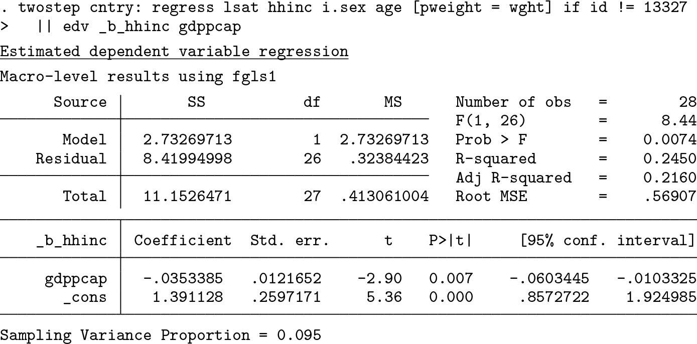
The finding of a potentially high-influence point for the microlevel regression in the case of Bulgaria can be further investigated using
In its simplest case, we need to replace only the microlevel command
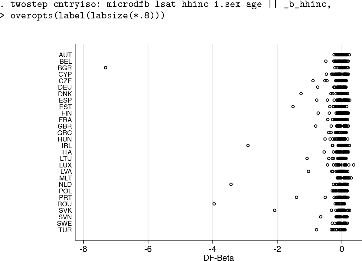
Box plots of DFBETAs for household income in the microlevel models by country
The figure shows box plots for the DFBETAs of household income in the microlevel models by country. The boxes themselves are barely visible because of one extraordinarily influential data point in the Bulgarian data. Issuing the command with the macro level option
reveals that this influential data point has the ID-number 13327. It may be worth noting that fitting the EDV model without that data point reduces the sampling variance proportion of the EDV model substantially, while considerably increasing the absolute value of the CLI term:
4.2.3 Macrolevel added-variable plot
The EDV model has indicated that the effect of household income on life satisfaction decreases with a country’s prosperity. Because the estimation of the CLI term relies on only 28 observations, we should study whether this effect merely results from few highinfluential data points. A standard tool to study this is the “added-variable plot”—also known as the partial-regression leverage plot, partial regression plot, or adjusted partial residual plot; see [R]
The
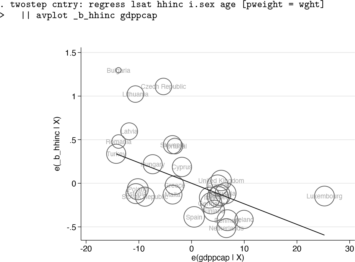
Added-variable plot for GDP per capita for the EDV model
The figure shows the added-variable plot for the macrolevel model of the coefficients of household income on GDP per capita. Because the macrolevel model has only one covariate, the plot is a bivariate scatterplot of the mean-centered regression coefficients on mean-centered GDP per capita. The regression line has the slope of the coefficient of the default EDV model, that is,
4.2.4 Macrolevel component-plus-residual plot
In the EDV model, the effect of household income on life satisfaction is estimated to linearly decrease with a country’s prosperity. However, it is possible that this CLI effect is actually nonlinear, so that the linear model provides a weak description for the way in which a country’s prosperity affects the effect of a person’s household income on their life satisfaction.
A common tool to investigate nonlinearity for multiple regression is the componentplus-residual plot—also known as the partial residual plot; see [R]
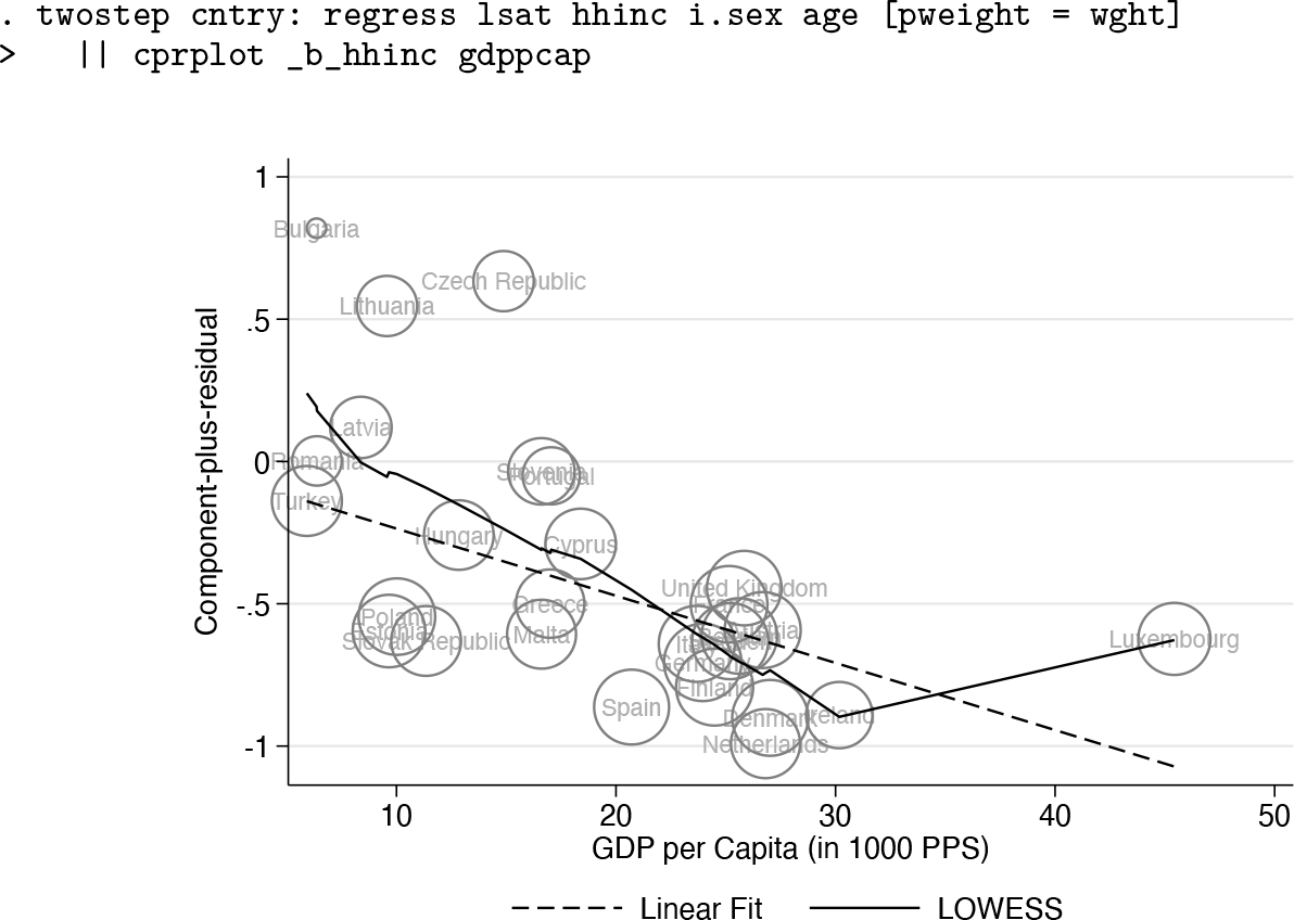
The component-plus-residual plot for GDP per capita for the EDV model
Because the macrolevel model has only one covariate, the figure is a bivariate scatterplot of the microlevel regression coefficients centered on the constant of the macrolevel regression on GDP per capita. The slope of the regression line is equal to the coefficient of
4.2.5 The regby plot
The macrolevel command

Regression lines of household income on life satisfaction by groups of GDP per capita
The command creates two groups of countries, first the countries with a GDP per capita below the median, second the countries above the median. The graph shows the regression slopes for household income in the microlevel models. Ideally, the slopes should be similar within each group and dissimilar between groups. To ease visual inspection, gray-shaded lines in the background show the slope for all countries. In this example, we see that the more affluent countries quite homogeneously have smaller coefficients for household income when compared with the poorer countries, whose coefficients are also more heterogeneous.
Variants of the plot allow users to control the grouping in various ways. This can be done by adding further macrovariables to macroindepvars or by using the options
4.3 Descriptive graphs
Instead of summarizing the results of the microlevel models with a regression at the second step, the two-step approach also suggests presenting the key parameters of the microlevel models graphically. In
In the following, however, we present the plot after tweaking it with some common options (figure 6):

Dot chart with options to tweak the look and feel
Apart from using Stata’s standard
The prime observation of figure 6 certainly is that all regression coefficients are larger than zero, with Bulgaria being exceptional in having both the largest effect of all countries and very large standard errors. Thus, personal affluence increases life satisfaction everywhere. We also see that the effect of household income on life satisfaction is on average a bit larger in the new EU member countries than in the older EU member countries. Finally, the coefficients vary slightly more among the new member countries than among the old member countries. Moreover, the confidence intervals tend to be larger in the former group. This creates suspicion of heteroskedasticity in the corresponding EDV model.
Note that the macrolevel command

4.4 Diagnostics
The two-step approach can also be used to study the formal assumptions invoked when performing multilevel analysis using the one-step approach. A standard way to check the normality assumption for a random coefficient in a mixed model is to predict the random effects and check their distribution with, say,

Quantiles of the predicted random effects for the household income coefficients against quantiles of a normal distribution
Note, though, that these random coefficients are estimated under the assumption that the parameterization of the model is correct. The two-step approach allows to check the same assumption without making a distributional assumption beforehand. Checking this assumption can be done by using a distributional diagnostic plot of the estimated parameters of the microlevel model. The

Quantiles of country-specific regression coefficients for household income against quantiles of a normal distribution
The figure reveals that there are more very small and very large effects of household income than what can be expected from a normal distribution. This corroborates the notion that the equivalent random-effects models may underestimate the standard error of the CLI.
Technically speaking, the distributional diagnostic plots are examples of
Another issue is the case of more fine-tuned regression diagnostics of the EDV model. As stated above,
This allows any kind of follow-up analysis on the macrolevel data. The EDV model can be invoked in the created dataset by using

Because
5 Conclusions
The two-step approach is a powerful addition to the statistical toolbox for analyzing hierarchical data. It is particularly useful if the number of microlevel observations within each macrolevel is large and the number of observations at the macrolevel is small. In such situations, the two-step approach can be used to estimate coefficients of CLIs and thus as an alternative to common one-step approaches such as cluster-corrected standard errors or fixed- and random-effects models on the pooled data. More importantly, however, the two-step approach gives direct access to less formal techniques of EDA that may provide additional insights into the research question at hand. The command
There are some limitations for the applied researcher when using
7 Programs and supplemental material
Supplemental Material, sj-zip-1-stj-10.1177_1536867X241257801 - Two-step analysis of hierarchical data
Supplemental Material, sj-zip-1-stj-10.1177_1536867X241257801 for Two-step analysis of hierarchical data by Johannes Giesecke and Ulrich Kohler in The Stata Journal
Footnotes
6 Acknowledgments
7 Programs and supplemental material
To install the software files as they existed at the time of publication of this article, type
Notes
References
Supplementary Material
Please find the following supplemental material available below.
For Open Access articles published under a Creative Commons License, all supplemental material carries the same license as the article it is associated with.
For non-Open Access articles published, all supplemental material carries a non-exclusive license, and permission requests for re-use of supplemental material or any part of supplemental material shall be sent directly to the copyright owner as specified in the copyright notice associated with the article.