A command to fit spatial stochastic frontier models with inefficiency spillovers

Abstract

The interdependence among decision-making units challenges the assumption of cross-sectional independence in traditional stochastic frontier models. Based on the seminal spatial Durbin specification for the frontier function, Galli (2023, Journal of the Royal Statistical Society, C ser., 72: 346-367) introduced inefficiency spillovers to measure neighborhood effects related to the inefficiency determinants. This article presents a new command, sfsd, that fits the comprehensive spatial stochastic frontier model that Galli (2023) proposed, accommodating various spatial and nonspatial specifications in both the frontier and the inefficiency equations. sfsd is the first command that includes different typologies of spatial spillovers in a stochastic frontier framework, facilitating the investigation of contemporary research topics such as agglomeration and technology diffusion at both the firm and the regional levels. The description, options, and illustrative examples for the command are outlined in this article.

Keywords

st0771 sfsd spatial stochastic frontier models spillover effects technical efficiency inefficiency spillovers

1 Introduction

Stochastic frontier analysis (sfa) is a widely used technique in assessing efficiency and productivity. The fundamental concept of sfa involves utilizing a production (or cost) frontier to measure the maximum (minimum) output (cost) achievable based on various inputs (cost determinants). Any deviation from this frontier can be attributed to inefficiency. Thus, decision-making units located on the frontier are considered completely efficient, indicating attainment of the maximum output with given inputs or the minimum cost for a specified level of output. The baseline stochastic frontier (sf) model was first introduced by Meeusen and van den Broeck (1977) and Aigner, Lovell, and Schmidt (1977). The original model incorporates a composite error term, which includes a classical random disturbance representing random shocks and a one-sided disturbance indicating inefficiency. Maximum likelihood techniques are commonly used to fit sf models, allowing for diverse assumptions regarding the error terms. With the global revolution in production processes and economic development, methodological and empirical research on efficiency analysis has flourished, expanding upon this foundational work by incorporating various enhancements to the baseline SF model.

With this wave, different packages for sfa have arisen, including the official commands frontier and xtfrontier for sfa on cross-sectional and panel-data: the community-contributed commands sfcross and sfpanel, which adapt to different distributional assumptions (Belotti et al. 2013); the community-contributed commands sfkk and xtsfkk, which fit endogenous sf models (Karakaplan 2017, 2022); and the community-contributed command sftt, which fits two-tier SF models (Lian, Liu, and Parmeter 2023). This article introduces a new command, sfsd, that fits the spatial SF model with inefficiency spillovers proposed by Galli (2023), which incorporates different spatial and nonspatial SF specifications.

The classical sf model assumes cross-sectional independence, which is inadequate considering the active interactions and feedback between decision-making units (Porter 1998; Delgado, Porter, and Stern 2014). This limitation may lead to biased estimates and invalid statistical inferences (Areal and Pede 2021). The spatial SF models literature emerged as a remedy, introducing spatial terms into sfa and taking advantage of spatial econometric techniques. In particular, the spatial lag of the dependent variable (spatial autoregressive [sar] term) and the spatial lag of the production inputs (spatial lag of X [slx] terms) introduced in the frontier function allow the capture of productivity and input spillovers, respectively. The former arises from the imitation of industry leaders by less efficient players, while the latter involves extensive improvements of input factors due to economic interactions, such as high-quality labor resulting from enterprise agglomeration. These global (sar) and local (slx) spatial mechanisms were first introduced in the frontier function by Glass, Kenjegalieva, and Sickles (2016). However, the spatial correlation of inefficiency remains unexplored.

To fill this gap, Galli (2023) proposed a comprehensive spatial sf model, which, for the first time, introduced spatial spillovers in the determinants of firms’ inefficiency, corresponding to traditional efficiency improvement paths such as knowledge spillovers and technology diffusion. Technically, Galli (2023) nested the specifications of Battese and Coelli (1995) and Glass, Kenjegalieva, and Sickles (2016) by merging 1) the spatial sf model with spillover effects in the frontier and 2) the inefficiency function, which models the mean of the inefficiency error term based on some exogenous inefficiency determinants, and further added the spatial lag of these inefficiency variables.

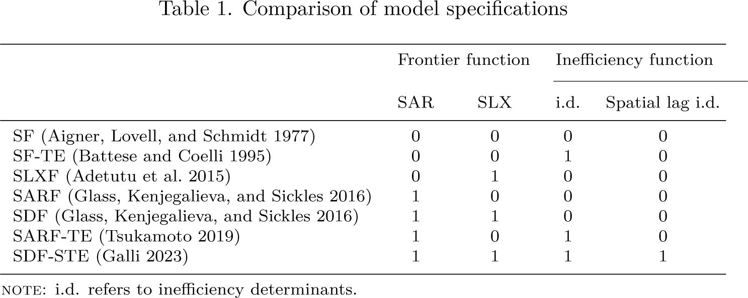
Table 1 provides a brief overview of the SF model’s evolution. Based on the classical model proposed by Aigner, Lovell, and Schmidt (1977), the SF model was expanded by Battese and Coelli (1995) to incorporate a model for the mean of the inefficiency error term. sf models were then further enriched by including spatial spillovers through sar and slx terms referring to the frontier function. Based on prior works, Galli (2023) gave full consideration to global and local spatial spillovers as well as inefficiency spillovers.

Table 1.
Comparison of model specifications

Frontier function Inefficiency function

SAR SLX i.d. Spatial lag i.d.

SF (Aigner, Lovell, and Schmidt 1977) 0 0 0 0

SF-TE (Battese and Coelli 1995) 0 0 1 0

SLXF (Adetutu et al. 2015) 0 1 0 0

SARF (Glass, Kenjegalieva, and Sickles 2016) 1 0 0 0

SDF (Glass, Kenjegalieva, and Sickles 2016) 1 1 0 0

SARF-TE (Tsukamoto 2019) 1 0 1 0

SDF-STE (Galli 2023) 1 1 1 1

	Frontier function	Inefficiency function
SF (Aigner, Lovell, and Schmidt 1977)	0	0	0	0
SF-TE (Battese and Coelli 1995)	0	0	1	0
SLXF (Adetutu et al. 2015)	0	1	0	0
SARF (Glass, Kenjegalieva, and Sickles 2016)	1	0	0	0
SDF (Glass, Kenjegalieva, and Sickles 2016)	1	1	0	0
SARF-TE (Tsukamoto 2019)	1	0	1	0
SDF-STE (Galli 2023)	1	1	1	1

NOTE: i. d. refers to inefficiency determinants.

In this article, we introduce a new command, sfsd, that estimates the comprehensive spatial SF specification of Galli (2023), which flexibly fits all the nested specifications mentioned in table 1, among others. Beyond considering various spillover mechanisms in the frontier and inefficiency functions, the sfsd command provides several postestimation tools. First, it is possible to calculate the spatially corrected inefficiency or efficiency scores following Kutlu, Tran, and Tsionas (2020). Second, the sfsd command allows computation of the direct, indirect, and total marginal effects related to the frontier variables and inefficiency determinants, as proposed by LeSage and Pace (2009). Finally, efficiency scores, along with their confidence intervals, are available following various specifications.

In practice, sfsd stands out as the only spatial SF command covering productivity input, and inefficiency spillovers. This method can be suitable for productivity and efficiency analysis at the microscale of enterprises and the macroscale of regions. Key issues of interest to policymakers, like imitation, agglomeration, knowledge spillovers, technology diffusion, and spatial networks, can be investigated with this approach. In particular, through spatial weight matrices, it is possible to account for various interaction logics of producers based on geographical, economic, and cultural distances, as well as others. In addition, given that the sfsd command fits a typical parametric model, different nested spatial specifications can be estimated starting from the general specification. In particular, the likelihood-ratio test can screen out the model that is most suitable for the data and reduce the risk of model misconfiguration.

The article is organized as follows: Section 2 provides a brief description of the model of Galli (2023); section 3 describes the syntax of sfsd, focusing on the main options; section 4 illustrates the command using simulated and real data; and finally, section 5 concludes.

2 Galli’s (2023) model

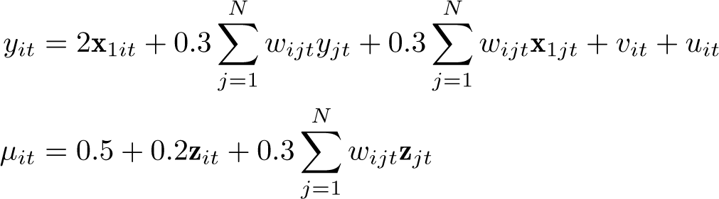
Spatial spillovers in traditional spatial SF models are conventionally limited to the frontier function (Glass, Kenjegalieva, and Sickles 2016). The spatial Durbin stochastic frontier model considering spatial effects in the inefficiency model (sDF-STE), introduced by Galli (2023), goes beyond this limitation by incorporating inefficiency spillovers related to the inefficiency determinants. A noteworthy contribution of this comprehensive spatial specification is that it allows exploration of the influence of the determinants of technical inefficiency in neighboring units on the inefficiency levels of specific units. This is achieved by adding the spatial lag of the inefficiency determinants in the inefficiency function, allowing for coverage of hot issues such as economic agglomeration and technology diffusion in the fields of enterprises and regional research. Technically, the SDF-STE model is defined as

y_{i t} = α_{1} + x_{1 i t} β + ρ \sum_{j = 1}^{N} w_{i j} y_{j t} + \sum_{j = 1}^{N} w_{i j} x_{1 j t} θ + v_{i t} - c u_{i t} (1)

(1)

u_{i} \overset{i . i . d .}{\sim} N^{+} (μ_{i t}, σ_{u}^{2}) (2)

(2)

μ_{i t} = α_{2} + x_{2 i t} γ + \sum_{j = 1}^{N} w_{i j} x_{2 j t} ϕ (3)

(3)

where

y_{i t}

represents the output or cost of productive unit singledollari = 1, \ldots ,Nsingledollar at time singledollart = 1, \ldots ,Tsingledollar and singledollar\alpha _1singledollar and singledollar\alpha _2singledollar are constants in the frontier and inefficiency mean functions respectively. singledollarX_{1it}singledollar is a singledollar1 \times k_1singledollar vector of input variables or cost determinants with an associated parameter vector singledollar\beta \lpar {k_1 \times 1} \rpar singledollar. singledollarw_{ij}singledollar denotes the generic element of the singledollarNT \times NTsingledollar block diagonal spatial weight matrix (singledollarWsingledollar), capturing spillover effects from unit singledollarjsingledollar to unit singledollarisingledollar.The parameter singledollar\rho singledollar and the singledollark_1 \times 1singledollar vector singledollar\theta singledollar are associated with the SAR and SLX terms, respectively, capturing global productivity spillovers and local input spillovers. singledollarv_{iL}singledollar is the random-error term following a normal distribution singledollar\left[ {v_{it}\mathop \sim \limits^{{\rm iid}} {\cal N}\lpar {0,\sigma_v^2 } \rpar } \right]singledollar. The inefficiency term singledollaru_itsingledollar follows a truncated normal distribution with mean singledollar\mu _{it}singledollar and variance singledollar\sigma _u^2 singledollar.In particular, when singledollarc = 1singledollar, a production frontier is specified; when singledollarc = -1singledollar ，we consider a cost frontier. The idea is that in the case of a cost frontier, inefficiency represents a cost increase, so inefficiency has to be summed to the frontier function. In contrast, for a production frontier, inefficiency is the decrease in the production level because of technical frictions, so the inefficiency term is subtracted from the frontier function.

Following the approach of Battese and Coelli (1995), variables explaining firms’ inefficiency levels are incorporated in the inefficiency mean function as shown in (3), where $x_{2 i t}$ is a $1 \times k_{2}$ vector of exogenous inefficiency determinants with corresponding parameter vector $γ (k_{2} \times 1)$ . The main feature of the SDF-sTE models consists of including the spatial lag of the inefficiency determinants to capture spillover effects arising from each determinant of neighboring firms’ efficiency through the $k_{2} \times 1$ vector of parameters $ϕ$ . Equations (1)–(3) constitute the foundational structure of the SDF-STE model, providing a framework for versatile combinations of spatial elements, including the SAR term, SLX term, and inefficiency spillover term.

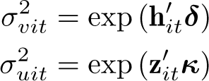
Moreover, uncontrolled observable heterogeneity in $v_{i t}$ and $u_{i t}$ can produce a bias in the parameter estimates of the frontier and inefficiency functions, threatening inference validity (Belotti et al. 2013). Following Caudill, Ford, and Gropper (1995) and Hadri (1999), we parameterize the variance of the idiosyncratic term and of the pretruncated inefficiency component as follows

\begin{aligned} σ_{v i t}^{2} = \exp (h_{i t}^{'} δ) \\ σ_{u i t}^{2} = \exp (z_{i t}^{'} κ) \end{aligned}

h_{i t}

and

z_{i t}

are exogenous variables affecting the distribution of the error term and inefficiency, respectively.

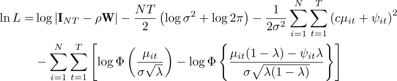
The model shown in (1)–(3) can be fit with a likelihood-based approach. The log likelihood function relies on the reparameterization $σ^{2} = σ_{u}^{2} + σ_{v}^{2}$ and $λ = (σ_{u}^{2}) / (σ_{u}^{2} + σ_{v}^{2})$ (with the constraints $σ^{2} > 0$ and $0 \leq λ \leq 1$ )and can be written as

\begin{aligned} \ln L = \log | I_{N T} - ρ W | - \frac{N T}{2} (\log σ^{2} + \log 2 π) - \frac{1}{2 σ^{2}} \sum_{i = 1}^{N} \sum_{t = 1}^{T} {(c μ_{i t} + ψ_{i t})}^{2} \\ - \sum_{i = 1}^{N} \sum_{t = 1}^{T} [\log Φ (\frac{μ_{i t}}{σ \sqrt{λ}}) - \log Φ {\frac{μ_{i t} (1 - λ) - ψ_{i t} λ}{σ \sqrt{λ (1 - λ)}}}] \end{aligned}

where

Φ

is the cumulative distribution function of the standard normal random variable

ψ_{i t} = υ_{i t} - c u_{i t} = y_{i t} - α_{1} - x_{1 i t} β - ρ \sum_{j = 1}^{N} w_{i j} y_{j t} - \sum_{j = 1}^{N} w_{i j} x_{1 j t} θ

，

μ_{i l} = α_{2} + x_{2 i t} γ + \sum_{j = 1}^{N} w_{i j} x_{2 i t} ϕ

, and

\log | I_{N T} - ρ W |

is the determinant of the Jacobian deriving from

(\partial ψ) / (\partial y)

.We can directly maximize the log-likelihood function

(\ln L)

above to estimate the model parameters.

As argued by LeSage and Pace (2009), the parameters $β$ and $γ$ in the SDF-STE model cannot be interpreted as marginal effects if the spatial lagged term of y is included Specifically, the marginal effects of the input variables and inefficiency determinants can be computed as partial derivatives as follows:

\frac{\partial y}{\partial x_{1_{r_{1}}}} = (I_{N T} - ρ W)^{- 1} (I_{N T} β + W θ) (4)

(4)

\frac{\partial u}{\partial x_{2_{r_{2}}}} = (I_{N T} - ρ W)^{- 1} (I_{N T} γ + W ϕ) (5)

(5)

$r_{1} = 1, \dots, k_{1}$ and $r_{2} = 1, \dots, k_{2}$ . Following LeSage and Pace (2009), we compute the marginal effects of the input variables and inefficiency determinants, respectively starting from the right-hand-side matrices of (4) and (5). Specifically, the direct effects are the average of the diagonal elements of these matrices; the indirect effects are the average of the nondiagonal elements of these matrices; and the total effects are the sum of direct and indirect effects. Technical details on the computation of the standard errors and t -values corresponding to the marginal effects can be found in LeSage and Pace (2009) and Glass, Kenjegalieva, and Sickles (2016).

3 The sfsd command

The sfsd command fits the spatial Durbin SF models with inefficiency spillovers introduced by Galli (2023).

3.1 Syntax

Estimation syntax

sfsd depvar [indepvars] [, i d(varname) t ime(varname) nocon stant cost

wxvars(varlist) mu(varlist [, noconstant]) wmuvars(varlist)

uhet(varlist [, nocons tant])vhet(varlist [, nocons tant]) wm at(wspec)

wym at(wyspec) wxm at(wxspec) wum at(wuspec)

norm alize(row | col | spectral | minmax) ini tial(matname)

mls earch(search_options) delve mlplot mlmode lopt(model_options)

mlmax opt(maximize_options) del missing nolog mex(varlist) meu(varlist)

mldisplay(display_options) genwvars constraints(constraints)

Version syntax

sfsd, ver sion

Replay syntax

Sfsd [, l evel(#)]

3.2 Options

3.2.1 Data structure

id(varname) specifies the cross-sectional ID variable of the production or cost unit. It is required for panel data.

time(varname) specifies the time variable. It must be specified for panel data. If time () is not specified, the data are assumed to be cross-sectional.

3.2.2 Frontier

noconstant suppresses the constant term (intercept) in the frontier function.

cost specifies that the model to be fit is a cost frontier model. By default, a production function is assumed.

wxvars (varlist) specifies spatially lagged independent variables in the frontier function.

3.2.3 Inefficiency

mu(varlist [, noconstant ]) specifies the explanatory variables in the inefficiency mean function.

wmuvars(varlist) specifies the spatially lagged variables in the inefficiency mean function.

3.2.4 Ancillary equations

uhet (varlist[, noconstant ]) specifies that the inefficiency component is heteroskedastic, with the variance expressed as a function of the covariates defined in varlist. Specifying noconstant suppresses the constant in this function.

vhet (varlist[, noconstant |) specifies that the idiosyncratic error component is heteroskedastic, with the variance expressed as a function of the covariates defined in varlist. Specifying noconstant suppresses the constant in this function.

3.2.5 Spatial weight matrices

wmat (wspec) specifies the spatial weight matrix. If specified, all spatial terms are based on the same weight matrix, defining wmat ( $W_{1}$ [ $W_{2} \dots W_{T}$ ] [, mata array]). By default, the weight matrices are Sp objects created by the Stata official command spmatrix. mata declares that weight matrices are Mata matrices. If one weight matrix is specified, it is assumed to be a time-invariant weight matrix. For time varying cases, T weight matrices should be specified in time order. Alternatively use array to declare that the spatial weight matrices are stored in an array. The time-invariant weight matrix is assumed if only one matrix is stored in the specified array. Otherwise, the keys of the array specify time information, and the values store time-specific spatial weight matrices.

wymat (wyspec) specifies the spatial weight matrices for the spatial lag of the dependent variable. The usage is the same as wmat ().

wxmat (wzspec) specifies the spatial weight matrices for the spatial lag of the independen variables in the frontier function. The usage is the same as wmat ().

wumat (wuspec) specifies the spatial weight matrices for the variables specified that are in wmuvars(). The usage is the same as wmat (). By default, spatial weight matrices in wmat() are used.

normalize(row | col | spectral | minmax) specifies the normalized method of spatial. weight matrices. By default, the command does not normalize the spatial weight matrices. normalize(row) is row normalization; normalize(col) is column normalization; normalize(spectral) is spectral normalization; and normalize (minmax) is minmax normalization.

3.2.6 Regression

initial(matname) specifies that matname is the initial value matrix.

mlsearch(search_options) specifies ml search options for searching initial values.

delve provides a regression-based methodology for searching for initial values. The default is to use ml search with default options.

mlplot specifies using ml plot to find better initial values.

mlmodelopt(model_options) controls ml model options; it is seldom used.

mlmaxopt (mazimize_options) controls ml maximize options; it is seldom used.

delmissing deletes the units with missing observations from spmatrix. If delmissing is not specified, a strongly balanced panel is required.

3.2.7 Reporting

nolog suppresses the display of the iterations.

mex(varlist) reports the total, direct, and indirect marginal effects of the variables in the frontier function.

meu(varlist) reports the total, direct, and indirect marginal effects of the variables in the inefficiency function.

mldisplay(display_options) controls the ml display options; it is seldom used.

genwvars generates the spatially lagged variables for the spatial terms in the frontier and inefficiency functions. It is required for implementing postestimation

3.2.8 Other

constraints (constraints) applies specified linear constraints for the fitted model.

3.3 Dependencies of sfsd

sfsd depends on the xtsfsp package contributed by Du, Orea, and Alvarez (2024). If not already installed, you can install it by typing

net install xtsfsp, from(/// “https://raw.githubusercontent.com/kerrydu/xtsfsp/refs/heads/main/xtsfsp/ado/”)

3.4 Postestimation commands after sfsd

The sfsd command allows postestimation. If the option genwvars is specified, the predict command can be used to compute linear predictions, efficiency scores, residuals, and the mean of the inefficiency distribution. If the SAR term is set when fitting the SF model, spatial-corrected inefficiencies or efficiencies using the Kutlu, Tran, and Tsionas (2020) estimator are available in postestimation. Moreover, following the definition of technical and cost inefficiency or efficiency proposed by Kumbhakar and Lovell (2000), sfsd and the related predict commands compute different types of inefficiency or efficiency scores depending on how the frontier is specified (technical efficiency is provided after the production frontier estimation, while cost efficiency for a cost frontier). The syntax of the predict command is

predict [type] newuar [if] [in] [，xb r esiduals mu u su te ste]

3.4.1 Statistic

xb, the default, calculates the linear prediction.

residuals calculates the composite residuals.

mu calculates the mean of the inefficiency distribution.

u computes the (technical or cost) inefficiency scores via $E (u ∣ ε)$ using the Jondrow et al. (1982) estimator.

su produces spatially corrected ineffciency following Kutlu, Tran, and Tsionas (2020).

te produces estimates of (technical or cost) efficiency via $E {\exp (- u) ∣ ε}$ (Battese and Coelli 1988).

ste produces estimates of spatial-corrected efficiency in the manner of Kutlu, Tran, and Tsionas (2020).

4 Examples

The sfsd command facilitates the estimation of various combinations of spatial terms in both the frontier and the inefficiency equations. Notably, sfsd, fitting the SDF-sTE model, is the first command considering inefficiency spillovers in SFA. Spatial weight matrices, whether time varying or time invariant, can be used according to user-defined settings. In this section, we initially conduct simulations using randomly generated panel data. Subsequently, we present an application case in macroeconomics using a real dataset from the Chinese tourism sector.

4.1 SDF-STE model with time-invariant spatial weight matrix

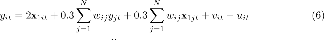
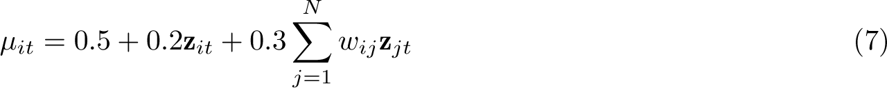
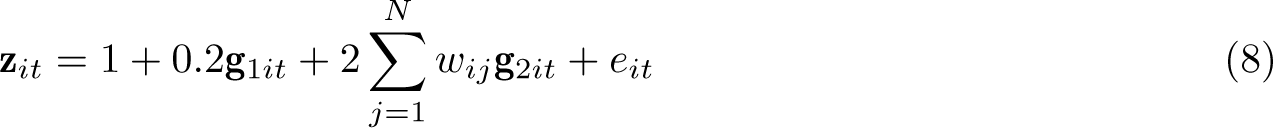
We first specify the SDF-sTE model through the following panel-data-generating process (DGP 1), where $t = 1, \dots, 20$ and $i = 1, \dots, 300$ . Importantly, all spatial spillover relationships are assumed to be time invariant, meaning that the elements $w_{i j t}$ of the spatial weight matrix $W_{t}$ remain unchanged throughout the period. The data are generated as follows:

y_{i t} = 2 x_{1 i t} + 0.3 \sum_{j = 1}^{N} w_{i j} y_{j t} + 0.3 \sum_{j = 1}^{N} w_{i j} x_{1 j t} + v_{i t} - u_{i t} (6)

(6)

μ_{i t} = 0.5 + 0.2 z_{i t} + 0.3 \sum_{j = 1}^{N} w_{i j} z_{j t} (7)

(7)

z_{i t} = 1 + 0.2 g_{1 i t} + 2 \sum_{j = 1}^{N} w_{i j} g_{2 i t} + e_{i t} (8)

(8)

$w_{i j}$ represents the element in the ith row and jth column of a randomly generated binary contiguity spatial weight matrix. This spatial weight matrix remains constant across the spatial components in (6)–(8), and it is row normalized. The term $υ_{i t} \overset{i . i . d .}{\sim} N (0, 0.2)$ denotes an independently and identically distributed (i.i.d.) normal rando variable. The inefficiency error term $u_{i} t$ follows a truncated normal distribution, as defined in (2), with variance $σ_{u}^{2} = 0.4$ and mean modeled as in (7). Additionally, $x_{1 i t}$ is a standard normal random variable, while Zit is generated based on a set of standard normal variables ( $g_{1 i t}$ ， $g_{2 i t}$ , and $e_{i t}$ ), as illustrated in (8).

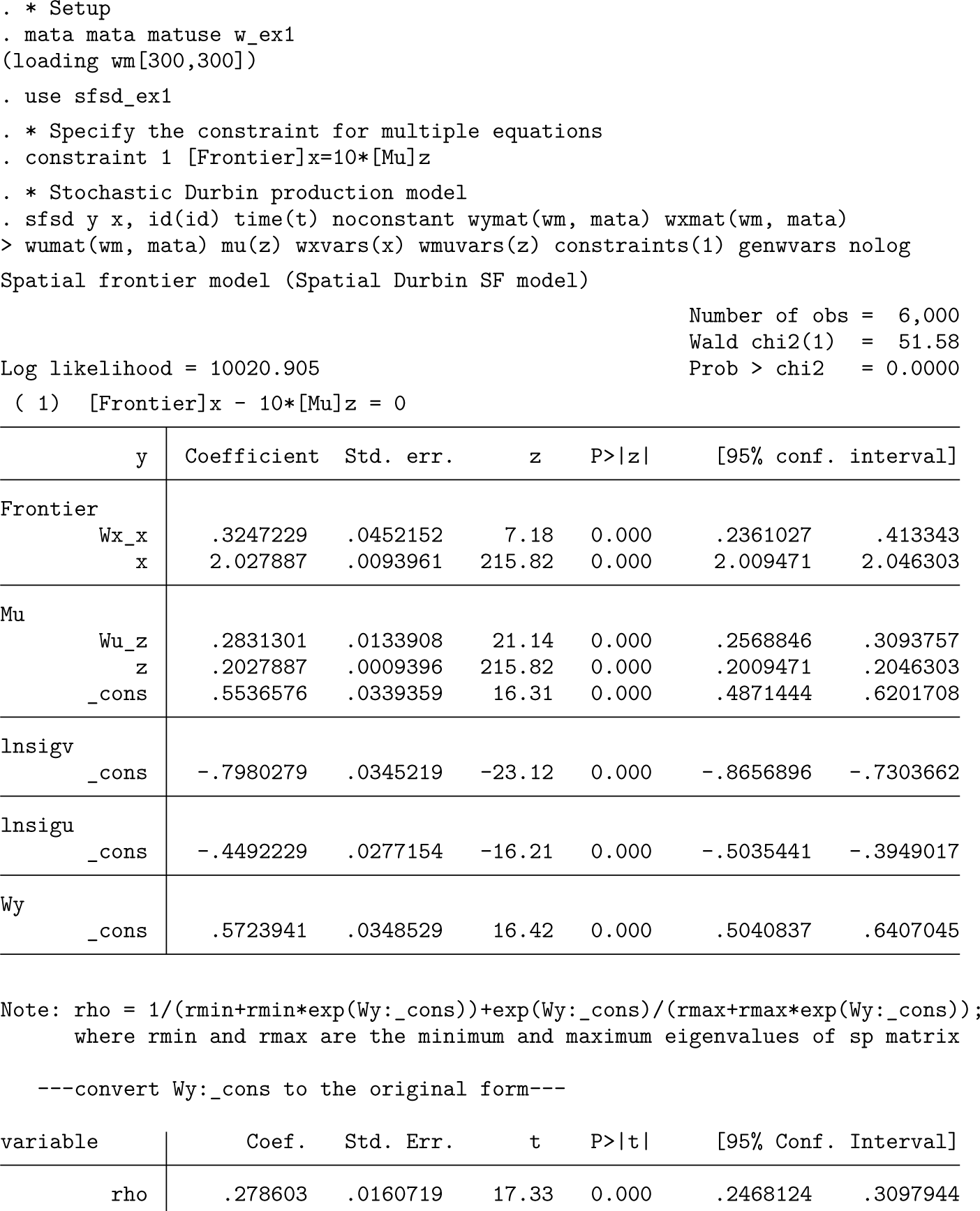
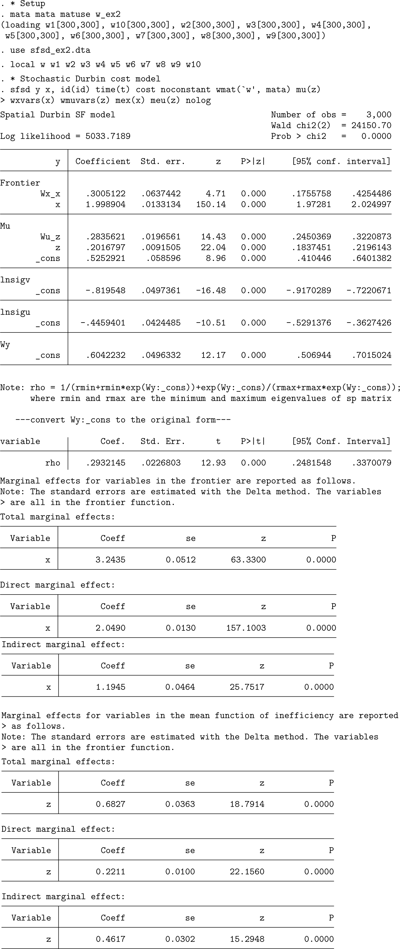
In empirical studies, SF models may be restricted by production or cost conditions. We perform constrained estimation on multiple equations in conjunction with the Stata constraint command to introduce how to set restrictions when using sfsd. In this simulation, the restriction example we have chosen imposes a quantitative relationship based on coefficients without any economic implications. Following (6) and (7)， we specify constraint 1 as the coefficient of $x_{1 i t}$ equal to 10 times the coefficient of $z_{i t}$ Then the option constraint(1) is specified when estimating with sfsd.

As is evident from the output, the Frontier and Mu panels display the estimates for the five parameters: Wx_x, X, Wu_z, z, and _cons, corresponding to the explanatory variables $θ$ ， $β$ ， $ϕ$ , γ，and $α_{2}$ in (6) and (7), respectively. The term _cons in the lnsigv and lnsigu bars represents the estimated natural logarithm of the square roots of $σ_{v}^{2}$ and $σ_{u}^{2}$ .The parameter associated with the SAR term is denoted as rho and is presented in another table along with the transformed function from the original matrix Additionally, if the same spatial weight matrix is specified for the cross-sectional spatial components, that is, $W_{y} = W_{x} = W_{u}$ , the aforementioned syntax is equivalent to using the wmat () option as follows:

sfsd y x, id(id) time(t) noconstant wmat(wm, mata) mu(z) ///

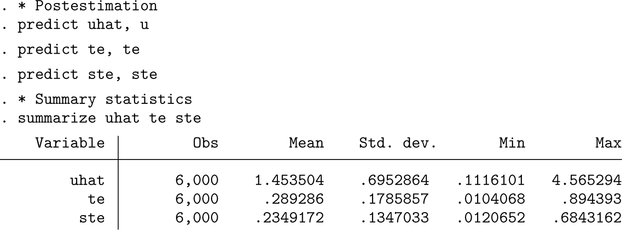
wxvars(x) wmuvars(z) constraints(1) genwvars nolog

4.1.1 Postestimation

Because we fit the SDF-STE model with the option genwvars, we use the predict command to obtain efficiency scores.

Options u and te are set to calculate the mean inefficiency and technical efficiency level for a production frontier. The ste option calculates spatial-corrected efficiency via $E_{i t} = \exp (- {\tilde{u}}_{i t})$ , following Kutlu, Tran, and Tsionas (2020), where $E_{i t}$ is the spatial corrected efficiency, ${\tilde{u}}_{i t} = E [u_{i t} | e_{i t}]$ , and $e_{i t} = v_{i t} - c u_{i t}$ . The resulting output provides a summary for the mean inefficiency uhat, technical efficiency te, and spatially corrected efficiency ste.

4.2 SDF-STE model with time-varying spatial weight matrix

Although the spatial relationships remain stable over time when using geographical distance, an alternative is available when using measures such as economic distance. The sfsd command allows users to construct time-varying spatial weight matrices. Additionally, in this section, we illustrate by estimating a cost function. In DGP 2, we generate panel data and a time-varying spatial weight matrix with $i = 1, \dots, 300$ and $t = 1, \dots, 10$ .Specifically, we replace (6)–(7) with the equations

\begin{aligned} y_{i t} = 2 x_{1 i t} + 0.3 \sum_{j = 1}^{N} w_{i j t} y_{j t} + 0.3 \sum_{j = 1}^{N} w_{i j t} x_{1 j t} + v_{i t} + u_{i t} \\ μ_{i t} = 0.5 + 0.2 z_{i t} + 0.3 \sum_{j = 1}^{N} w_{i j t} z_{j t} \end{aligned}

where

w_{i j t}

varies over time and the remaining parameters are set as before. The time varying spatial weight matrix is specified by stacking the cross-sectional spatial weight matrices in the wmat () option in order of time. In this example, 10 spatial weight matrices

W_{t}

，with

t = 1, \dots, 10

, are placed in order in local w, which is later specified in the wmat () option, taken from Mata, and combined into the target time-varying matrix.

We incorporate the cost option to estimate a cost function. We also include the meu(x) and meu(z) options to calculate the marginal effects of the input variable (x) and the inefficiency determinant (z). The resulting output presents total marginal effects, further decomposing them into direct and indirect marginal effects along with their corresponding standard errors.

4.3 Empirical example

Spatial SF models have been widely used in macroeconomic analyses (see Orea, Alvarez and Jamasb [2018]and Gude, Alvarez, and Orea [2018]). In this section, we apply the SDF-STE model to real data, exploring the case of the developing Chinese tourism industry by estimating the effect of tourism flows and their spatial spillovers on Chinese cities’ economic efficiency. The idea is that tourism flows both at the destination and from adjacent cities may impact cities economic performance.

On the one hand, Copeland (1991) explained that if the expanding tourism industry raises the price of nontradable goods, production factors will shift from manufacturing to nontradable sectors. This shift results in a relative decline of the manufacturing industry, ultimately harming the economic production frontier. Similarly, expanding tourism in neighbors attracts production factors not only from the local industry but also from the industry in adjacent cities because of the low shipping costs due to geographical advantages. Thus, the tourism spillover effect may also crowd out local manufacturing inputs, negatively impacting the production frontier. On the other hand, the positive stimulation of economic efficiency corresponds to the knowledge spillover, such as preferences for local manufacturers, conveyed by tourists as mentioned by Marrocu and Paci (2011). In contrast, tourists visiting adjacent cities have fewer opportunities to exchange adequate information; thus, the spillover on economic efficiency can be less effective.

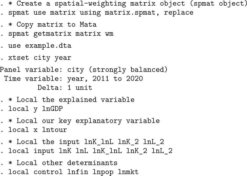
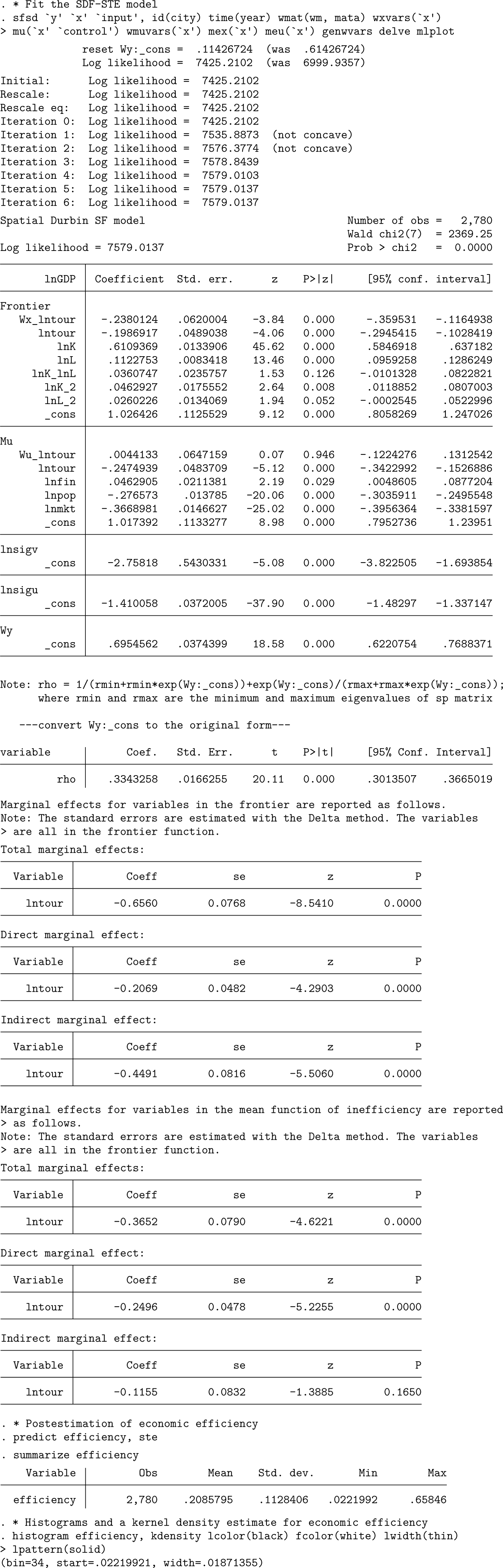
Raw data on 278 Chinese cities from 2011 to 2020 have been collected from the CEIC database. These data include gross domestic product (lnGDP)，the number of tourists covering Chinese and foreign tourists (lntour), capital investments (lnK), the number of employees (lnL), the financial efficiency represented by the ratio of loans to deposits (lnfin), the city size defined by the permanent population at the end of the year (lnpop), and the marketization level specified by the reciprocal of general public budget expenditure as a share of gross domestic product (lnmkt). In particular lnGDP has been adjusted to the constant price in 2001, and the stock of capital has been calculated using the perpetual inventory method. While labor and capital are transformed using the second-order translog function as inputs to model the frontier function with the natural log of lnGDP as the dependent variable, we include the natural log of lntour in the frontier and inefficiency mean functions along with its spatial lag to measure the effect of the city’s as well as neighbors’ tourism flows on the urban economy. Moreover, we also include other inefficiency determinants (lnfin, lnpop, lnmkt) in the inefficiency mean model as controls.

First, we use the command spmat (Drukker et al. 2013) to read the spatial weight matrix from the spmat object and transfer the spatial weight matrix wm into the Mata environment before estimation. The spatial weight matrix is generated as the inverse of the square distance between cities and truncated at 1,000 km. Then, to facilitate convergence, we include the delve and mlplot options. In addition, we specify the mex, meu, and genwvars options to report the results of the marginal effects for lntour and perform postestimation, respectively.

As shown in the results, developing tourism is found to harm the economic frontier but benefit economic efficiency. Considering spatial correlation, spillovers from neighbors’ tourism have a significantly negative impact on the local production frontier, while they have no significant impact on economic efficiency. All the results are consistent with the theoretical analysis conducted in previous literature.

The estimated marginal effects for lntour suggest that, in the frontier function, indirect effects from tourism in surrounding areas equal -0.4491, while direct effects stand at -0.2069. Therefore, the adverse effects of tourism on the productivity of Chinese cities are greater in magnitude for impacts originating from neighbors than local internal effects. On the other hand, the total marginal effect of tourism on the mean inefficiency level of Chinese cities (equal to -0.3652) is mainly directed by local tourism with a direct effect of -0.2496 and a nonsignificant indirect effect of -0.1155.

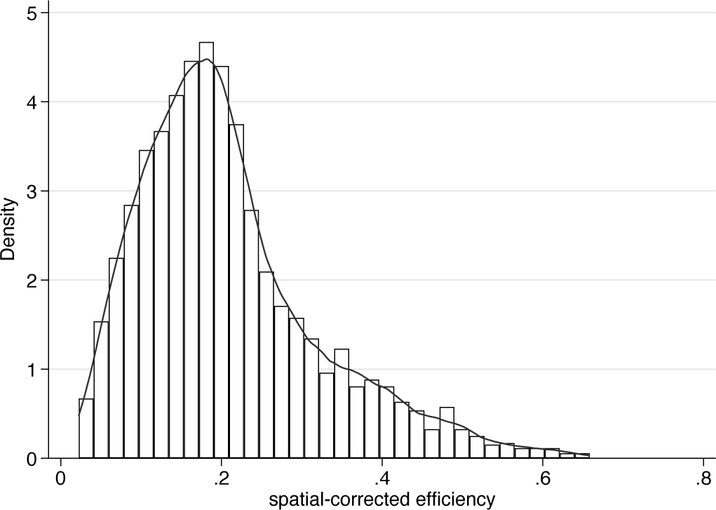
As an example of postestimation, figure 1 shows the histogram of spatially corrected efficiency, highlighting the typical efficiency distribution for developing countries with considerable production volumes but relatively low economic efficiency.

Figure 1.

Histogram of spatially corrected efficiency scores.

Technically, the different typologies of spatial spillovers detected in this empirical application underscore the importance of comprehensively considering various spatial mechanisms in the framework of SFA. In this empirical application, failure to do so may result in policymakers overlooking the adverse spillover effects on the economic frontier. In summary, the SDF-STE model proposed by Galli (2023) and fit using the sfsd command is a powerful tool for considering both spatial effects and efficiency analyses.

5 Conclusions

In this article, we presented the command sfsd, which fits the comprehensive spatial SF model with inefficiency spillovers proposed by Galli (2023), contributing to advancing empirical research in the productivity and efficiency analysis framework using Stata. sfsd supports the postestimation of various efficiency scores, including the spatial-corrected efficiency and inefficiency index proposed by Kutlu, Tran, and Tsionas (2020). Users can thoroughly explore different combinations of spatial spillovers among decision-making units using sfsd. We demonstrate the estimation capabilities of sfsd by means of simulated data and use a real dataset on Chinese tourism to explore the spillover effect as an empirical example.

Future commands for spatial SF models should consider handling possible endogeneity issues related to the input or environmental variables in the style of Kutlu, Tran, and Tsionas (2020) and including fixed effects as proposed by Galli (2024).

6 Acknowledgments

We are grateful to Federico Belotti, Silvio Daidone, Giuseppe Ilardi, and Vincenzo Atella (2013) for the sfcross and sfpanel package; Mustafa U. Karakaplan (2017) for the sfkk package; and Jan Ditzen, William Grieser, and Morad Zekhnini (2023) for the nwxtregress package, which inspired our design of the sfsd command. Kerui Du is thankful for the financial support from the National Natural Science Foundation of China (Grant no. 72074184)

7 Programs and supplemental material

To install the software files as they existed at the time of publication of this article type

Supplemental Material

sj-dta-1-stj-10.1177_1536867X251322970 - Supplemental material for A command to fit spatial stochastic frontier models with inefficiency spillovers

Supplemental material, sj-dta-1-stj-10.1177_1536867X251322970 for A command to fit spatial stochastic frontier models with inefficiency spillovers by Kerui Du, Federica Galli, Luojia Wang in The Stata Journal

Supplemental Material

sj-txt-2-stj-10.1177_1536867X251322970 - Supplemental material for A command to fit spatial stochastic frontier models with inefficiency spillovers

Supplemental material, sj-txt-2-stj-10.1177_1536867X251322970 for A command to fit spatial stochastic frontier models with inefficiency spillovers by Kerui Du, Federica Galli, Luojia Wang in The Stata Journal

Footnotes

About the authors

Kerui Du is an associate professor at the School of Management, Xiamen University, China. His primary research interests include applied econometrics, energy, and environmental economics.

Federica Galli is a postdoctoral research fellow in economic statistics at the Department of Statistical Sciences “Paolo Fortunati” of the University of Bologna, Italy.

Luojia Wang (corresponding author) is a doctoral student in technical economy and management at the School of Management, Xiamen University, China.

References

Adetutu

Glass

A. J.

Kenjegalieva

Sickles

R. C.

. 2015.The effects of efficiency and TFP growth on pollution in Europe: A multistage spatial analysis. Journal of Productivity Analysis 43: 307–326. 10.1007/s11123-0140426-7.

Aigner

D. J.

Lovell

C. A. K.

Schmidt

. 1977. Formulation and estimation of stochastic frontier production function models. Journal of Econometrics 6: 21–37 10.1016/0304-4076(77)90052-5.

Areal

F. J.

Pede

V. O.

. 2021. Modeling spatial interaction in stochastic frontier analysis. Frontiers in Sustainable Food Systems 58: art. 673–039. 103389/fsufs.2021.673039.

Battese

G. E.

Coelli

T. J.

. 1988. Prediction of firm-level technical efficiencies with a generalized frontier production function and panel data. Journal of Econometrics 38: 387399. 10.1016/0304-4076(88)90053-X.

______. 1995. A model for technical inefficiency effects in a stochastic frontier production function for panel data. Empirical Economics 20: 325–332. 10.1007/BF01205442.

Belotti

Daidone

Ilardi

Atella

. 2013. Stochastic frontier analysis using Stata. Stata Journal 13: 719–758. 10.1177/1536867X1301300404.

Caudill

S. B.

Ford

J. M.

Gropper

D. M.

. 1995. Frontier estimation and firm-specific inefficiency measures in the presence of heteroscedasticity. Journal of Business and Economic Statistics 13: 105–111. 10.1080/07350015.199510524583.

Copeland

B. R

. 1991. Tourism, welfare and de-industrialization in a small open economy. Economica 58: 515–519. 10.2307/2554696.

Delgado

Porter

M. E.

Stern

. 2014. Clusters, convergence, and economic performance. Research Policy 43: 1785–1799. 10.1016/j.respol.201405.007.

10.

Ditzen

, W. Grieser, and M. Zekhnini. 2023. nwxtregress: Network regressions in Stata. GitHub. https://janditzen.github.io/nwxtregress/ .

11.

Drukker

D. M.

Peng

Prucha

I. R.

Raciborski

. 2013. Creating and managing spatial-weighting matrices with the spmat command. Stata Journal 13: 242–286 10.1177/1536867X1301300202.

12.

Orea

Alvarez

I. C.

. 2024. Fitting spatial stochastic frontier models in Stata. Stata Journal 24: 402–426. 10.1177/1536867X241276109.

13.

Galli

. 2023. A spatial stochastic frontier model introducing inefficiency spillovers. Journal of the Royal Statistical Society, C ser., 72: 346–367. 101093/jrsssc/qlad012.

14.

____. 2024. Accounting for unobserved individual heterogeneity in spatial stochastic frontier models: The case of Italian innovative start-ups. Spatial Economic Analysis 19: 620–645. 10.1080/17421772.2024.2306953.

15.

Glass

A. J.

Kenjegalieva

Sickles

R. C.

. 2016. A spatial autoregressive stochastic frontier model for panel data with asymmetric efficiency spillovers. Journal of Econometrics 190: 289–300. 10.1016/jjeconom.2015.06.011.

16.

Gude

Alvarez

Orea

. 2018. Heterogeneous spillovers among Spanish provinces: A generalized spatial stochastic frontier model. Journal of Productivity. Analysis 50: 155–173. 10.1007/s11123-018-0540-z.

17.

Hadri

. 1999. Estimation of a doubly heteroscedastic stochastic frontier cost function. Journal of Business and Economic Statistics 17:359–363. 10.108007350015.1999.10524824.

18.

Jondrow

Lovell

C. A. K.

Materov

I. S.

Schmidt

. 1982. On the estimation of technical inefficiency in the stochastic frontier production function model. Journal of Econometrics 19: 233–238. 10.1016/0304-4076(82)90004-5.

19.

Karakaplan

M. U

. 2017. Fitting endogenous stochastic frontier models in Stata. Stata Journal 17: 39–55. 10.1177/1536867X1701700103.

20.

_____. 2022. Panel stochastic frontier models with endogeneity. Stata Journal 22: 643–663. 10.1177/1536867X221124539.

21.

Kumbhakar

S. C.

Lovell

C. A. K.

. 2000. Stochastic Frontier Analysis. Cambridge, Cambridge University Press. 10.1017/CBO9781139174411.

22.

Kutlu

Tran

K. C.

Tsionas

M. G.

. 2020. A spatial stochastic frontier model with endogenous frontier and environmental variables. European Journal of Operational Research 286: 389–399. 10.1016/j.ejor.2020.03.020.

23.

LeSage

Pace

R. K.

. 2009. Introduction to Spatial Econometrics . Boca Raton FL: Chapman and Hall/CRC. 10.1201/9781420064254.

24.

Lian

Liu

Parmeter

C. F.

. 2023. Two-tier stochastic frontier analysis using Stata. Stata Journal 23: 197–229. 10.1177/1536867X231162033.

25.

Marrocu

Paci

. 2011. They arrive with new information. Tourism flows and production efficiency in the European regions. Tourism Management 32: 750–758 10.1016/j.tourman.2010.06.010.

26.

Meeusen

van den Broeck

. 1977. Efficiency estimation from Cobb-Douglas production functions with composed error. International Economic Review 18: 435–444. 10.2307/2525757.

27.

Orea

Alvarez

I. C.

Jamasb

. 2018. A spatial stochastic frontier model with omitted variables: Electricity distribution in Norway. Energy Journal 39: 93–116. 10.5547/01956574.39.3.lore

28.

Porter

. 1998. Clusters and the new economics of competition. Harvard Business Review 76:77–90.

29.

Tsukamoto

. 2019. A spatial autoregressive stochastic frontier model for panel data incorporating a model of technical inefficiency. Japan and the World Economy 50: 66–77. 10.1016/j.japwor.2018.11.003.

Supplementary Material

Please find the following supplemental material available below.

For Open Access articles published under a Creative Commons License, all supplemental material carries the same license as the article it is associated with.

For non-Open Access articles published, all supplemental material carries a non-exclusive license, and permission requests for re-use of supplemental material or any part of supplemental material shall be sent directly to the copyright owner as specified in the copyright notice associated with the article.

0.00 MB

0.14 MB

0.00 MB

	Frontier function		Inefficiency function
	SAR	SLX	i.d.	Spatial lag i.d.
SF (Aigner, Lovell, and Schmidt 1977)	0	0	0	0
SF-TE (Battese and Coelli 1995)	0	0	1	0
SLXF (Adetutu et al. 2015)	0	1	0	0
SARF (Glass, Kenjegalieva, and Sickles 2016)	1	0	0	0
SDF (Glass, Kenjegalieva, and Sickles 2016)	1	1	0	0
SARF-TE (Tsukamoto 2019)	1	0	1	0
SDF-STE (Galli 2023)	1	1	1	1