ge_gravity2: A command for solving universal gravity models

Abstract

Abstract.

In this article, we describe an algorithm for computing counterfactual trade flows, prices, output, and welfare in a large class of general equilibrium trade models. We introduce a command called ge_gravity2, which allows users to perform these computations in Stata. This command extends the existing ge_gravity command by allowing users to compute the general equilibrium effects of changes in trade policy in positive supply elasticity models. It can be used to solve any model that falls into the class of universal gravity models as defined by Allen, Arkolakis, and Takahashi (2020, Journal of Political Economy 128: 393-433).

Keywords

st0790 ge gravity2 general equilibrium structural gravity universal gravity model positive supply elasticity trade policy

1 Introduction

In economics, the use of simulation models to analyze the impact of trade policies on trade flows is of great importance to policymakers and researchers alike. An early way of simulating structural gravity models in Stata was an ingenious procedure known as GEPPML, which was proposed by Anderson, Larch, and Yotov (2018), who repurposed a Poisson pseudo-maximum-likelihood estimator to conduct general equilibrium simulations. Zylkin (2019) later developed ge_gravity, an independent command that can be used to simulate how trade flows and welfare respond to changes in bilateral trade costs, using the general equilibrium model and algorithm described by Baier, Yotov, and Zylkin (2019). In this article, we introduce a new command called ge_gravity2 (Campos, Reggio, and Timini 2024).

The ge_gravity2 command is designed to solve a more general class of models because it applies to economic models that have a positive aggregate supply elasticity, whereas the ge_gravity command is restricted to models in which the aggregate supply elasticity is 0. Another way in which the new command improves on the previous ge_gravity command is that it can be used to simulate the effects of changes in technology parameters and trade balance parameters.

The ge_gravity2 command allows users to explore the effects of trade policy in trade models where the aggregate supply of goods is an increasing function of output prices and, more generally, to simulate a very wide range of economic geography models that combine aggregate demand and supply equations with standard market clearing conditions. This new command can be used to simulate the global effects of changes in trade frictions and supply shifters in any model that falls within the “universal gravity” framework described by Allen, Arkolakis, and Takahashi (2020).

As stated by Allen, Arkolakis, and Takahashi (2020), a model belongs to the class of universal gravity models if an aggregate good is traded across locations and if it satisfies six specific economic conditions or properties: 1) bilateral trade frictions of the “iceberg” type, 2) constant elasticity of substitution in aggregate demand, 3) constant elasticity of substitution in aggregate supply, 4) market clearing, 5) exogenous trade deficits, and 6) a choice of numeraire. These six conditions provide sufficient structure to fully describe all general equilibrium interactions of trade flows, incomes, and real output prices in terms of the elasticity of aggregate demand and supply.

The universal gravity framework encompasses a wide variety of models, including those of Armington (1969), Anderson (1979), Anderson and van Wincoop (2003), Krug- man (1980), Eaton and Kortum (2002), Melitz (2003), di Giovanni and Levchenko (2013), Allen and Arkolakis (2014), Redding (2016), and Redding and Sturm (2008). On the other hand, many prominent models do not fall into the category of universal gravity models. These typically include models where there are multiple factors of production with varying intensities, where trade deficits evolve endogenously, or where demand and supply elasticities are not constant. In addition, models that include additional sources of revenue, such as tariffs, generally do not fit into the universal gravity framework except in special circumstances.

The article is organized as follows. In section 2, we present a prototypical trade model with positive supply elasticity that serves as an example of the kind of models that can be simulated using the ge_gravity2 command. We then state the properties that characterize the universal gravity framework and show that the prototypical trade model belongs to this class of models. Next we show how to derive the system of equations that can be used to compute comparative statics and present an algorithm that solves for general equilibrium price changes for all universal gravity models. The system of equations (slightly) generalizes the one considered by Allen, Arkolakis, and Takahashi (2020) in that it applies to unbalanced trade while allowing for changes in bilateral trade costs, exogenous trade costs, and parameters in the production function. The algorithm we present is fully global in that it solves the nonlinear system of equations rather than a local approximation to that system. The algorithm uses a fixed-point procedure a la Alvarez and Lucas (2007) that converges to the solution of the system of equations almost instantaneously in most applications.

In section 3, we present the syntax of the ge_gravity2 command, the options that are available to the user, and the results stored by the command after its execution. Despite its broader scope, the usage of the ge_gravity2 command remains very similar to that of ge_gravity, making it easy for users of the previous command to seamlessly transition to the new command. The new command is backward compatible with ge_gravity and will produce the same results when the supply elasticity is set to zero. Compared with the current version of ge_gravity, ge_gravity2 allows additional inputs and outputs and stores several matrices that can be inspected by the user after execution.

Section 4 demonstrates the use of the command through three examples. The first example demonstrates the basic use of the command by showing how to perform an ex ante analysis of the effects of a trade agreement. The second example demonstrates the use of the command with the by prefix by going through an example inspired by Campos, Reggio, and Timini (2023) that calculates the evolution of welfare costs associated with trade policies in Spain during the Franco regime. The third example shows how the command can be used to simulate a scenario in which trade costs remain unchanged but a country’s productivity increases, which in general equilibrium affects welfare and other economic variables for all countries in the world.

We conclude in section 5 and show how to install the command in section 7. In the online appendix, we derive various results that are used in the article but are too long to include in the main text.

2 Economic theory and methods

2.1 A prototypical trade model with a positive supply elasticity

There are N locations, denoted by the subscript i or j. Sending goods from i to j incurs an iceberg trade cost, denoted by τ _ij ≥ 1. Goods are produced by combining immobile labor with intermediate inputs. As in the model of Eaton and Kortum (2002), the production function is a Cobb-Douglas function with constant returns to scale, where ζ denotes the share of labor (L_i) in costs, 1 — ζ denotes the share of intermediate inputs (M_i), and A_i > 0 denotes labor productivity:

Q_{i} = (A_{i} L_{i})^{ζ} M_{i}^{1 - ζ}

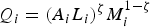
Intermediates are assumed to be the same bundle of goods as those entering final consumption so that the price index for intermediates for each firm is the price index taken over all goods.¹ We denote this price index by Pi.

Assuming perfect competition, the price of output at location i is given by

p_{i} = \bar{κ} (w_{i} / A_{i})^{ζ} P_{i}^{1 - ζ}

where

\bar{κ} > 0

is a constant and w_i is the wage rate. The value of output at the origin is Y_i = p_iQ_i. Because labor is the only factor of production and profits are zero, all output is distributed to workers. This leads to the macroeconomic accounting identity

Y_{i} = p_{i} Q_{i} = w_{i} L_{i}

which means that Y_i is simultaneously a measure of the value of production, labor income, and total income at a location.

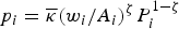
Because of arbitrage in the goods markets, the price paid at a destination j for a good that is shipped from the origin i is

p_{i j} = τ_{i j} p_{i} (1)

(1)

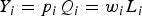
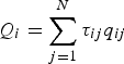
The amount of goods that reach the destination j after subtracting the iceberg cost is denoted by q_ij. The expenditure on this good, valued at prices at the destination, is

X_{i j} = p_{i j} q_{i j}

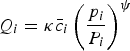
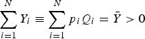
Equilibrium requires that output markets clear, that is, that prices and quantities adjust so that output Q_i at each location equals the aggregate demand from all locations, including iceberg costs:

Q_{i} = \sum_{j = 1}^{N} τ_{i j} q_{i j} (2)

(2)

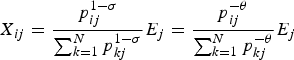
At each location, there is a representative consumer who supplies labor inelastically and whose entire income comes from labor income. This consumer values varieties of goods according to a constant elasticity of substitution (CES) function that aggregates goods from all origins, as in the models of Armington (1969), Anderson (1979), and Anderson and van Wincoop (2003). The elasticity of substitution is denoted by σ > 1. The optimization problem of the consumer leads to the well-known result that expenditure on goods from different origins can be expressed as

X_{i j} = \frac{p_{i j}^{1 - σ}}{\sum_{k = 1}^{N} p_{k j}^{1 - σ}} E_{j} = \frac{p_{i j}^{- θ}}{\sum_{k = 1}^{N} p_{k j}^{- θ}} E_{j} (3)

(3)

where expenditure E_j is defined by

E_{j} \equiv Σ_{i} X_{i j}

and

θ \equiv σ - 1 > 0

. The parameter θ is known as the trade elasticity.

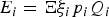
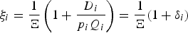
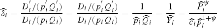
Trade deficits are exogenous. Expenditure at any location i is expressed as a multiple of the value of output as

E_{i} = Ξ ξ_{i} p_{i} Q_{i} (4)

(4)

where

Ξ \equiv \frac{\sum_{i} p_{i} Q_{i}}{\sum_{i} ξ_{i} p_{i} Q_{i}}

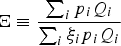
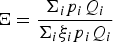
The parameter ξ _i > 0 is location specific, and the parameter Ξ is common to all locations. This way of specifying trade deficits ensures that the sum of exports from all locations always equals the sum of imports from all locations. In the special case where ξ _i = 1 for all i (which also implies Ξ = 1), the trade deficits of all locations are exactly 0. On the other hand, if some ξ _i ≠ 1, then trade is not balanced at all locations. The trade deficit at location i can then be expressed as

D_{i} \equiv E_{i} - Y_{i} = (Ξ ξ_{i} - 1) p_{i} Q_{i}

Summing trade deficits over all i, we have

\sum_{i = 1}^{N} D_{i} = Ξ (\sum_{i = 1}^{N} ξ_{i} p_{i} Q_{i} - \sum_{i = 1}^{N} p_{i} Q_{i}) = \frac{Σ_{i} p_{i} Q_{i}}{Σ_{i} ξ_{i} p_{i} Q_{i}} (\sum_{i = 1}^{N} ξ_{i} p_{i} Q_{i} - \sum_{i = 1}^{N} p_{i} Q_{i}) = 0

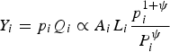
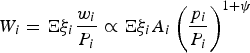
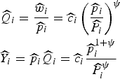
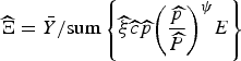
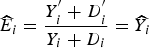
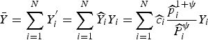
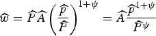
In this model, output (Qi), income (Y_i), and welfare (W_i) are proportional to real output prices p_i/P_i raised to powers of the supply elasticity, which is defined as $ψ \equiv (1 - ζ) / ζ$ .² The real output price p_i/P_i is also a measure of terms of trade because it expresses the price obtained for exports of location i in terms of prices paid for imports at location i (including imports from itself). Using the notation “ $\propto$ ” to express proportionality, we have that

Q_{i} \propto \frac{w_{i}}{p_{i}} L_{i} \propto A_{i} L_{i} {(\frac{p_{i}}{P_{i}})}^{ψ} (5)

(5)

Y_{i} = p_{i} Q_{i} \propto A_{i} L_{i} \frac{p_{i}^{1 + ψ}}{P_{i}^{ψ}}

W_{i} = Ξ ξ_{i} \frac{w_{i}}{P_{i}} \propto Ξ ξ_{i} A_{i} {(\frac{p_{i}}{P_{i}})}^{1 + ψ}

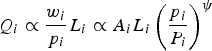
The first of these results shows why $ψ$ is called a supply elasticity. Holding all other variables constant, the elasticity of output with respect to the price p_i is given by

\frac{\partial In Q_{i}}{\partial In p_{i}} = ψ \geq 0

The prototypical model described in this section falls into the more general class of models that Allen, Arkolakis, and Takahashi (2020) define as the universal gravity framework. We now turn to the characterization of this more general framework and how it can be used to solve for the price ratio p_i/P_i, which—together with the supply elasticity ψ—is a sufficient statistic for real wages and ultimately welfare in the prototypical trade model.

2.2 The universal gravity framework

Models that are part of the universal gravity framework satisfy six properties. We list them briefly and refer the reader to the article by Allen, Arkolakis, and Takahashi (2020) for a more detailed discussion.

Property 1 (arbitrage in goods markets). The bilateral price is equal to the product of the output price and a bilateral scalar (iceberg cost),

p_{i j} = τ_{i j} p_{i}

where

τ_{i j} \in R_{+ +} \cup {\infty}

Property 2 (CES aggregate demand). Expenditure at every location j can be written as

E_{j} = {(\sum_{i = 1}^{N} p_{i j}^{- 0})}^{- \frac{1}{θ}} E_{j}

where

E_{j}

is real expenditure at location j and the associated price index is

P_{j} \equiv (Σ_{i} p_{i j}^{- θ})^{- \frac{1}{θ}}

. The parameter

θ \in R_{+ +}

is called the demand elasticity or trade elasticity.

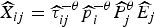
Because of Shephard’s lemma, property 2 implies that the value of trade flows, defined as X_ij = p_ijq_ij (where q_ij is the real value of goods arriving at location j and p_ij is their price at location j), can be written as a function of prices and expenditure as follows:

X_{i j} = \frac{p_{i j}^{- θ}}{\sum_{k} p_{k j}^{- θ}} E_{j}

Note that by summing this equation over i, we also obtain

\sum_{i} X_{i j} = E_{j}

Property 3 (CES aggregate supply). Output at each location can be written as

Q_{i} = κ {\bar{c}}_{i} {(\frac{p_{i}}{P_{i}})}^{ψ}

where κ > 0. The so-called supply shifters are strictly positive;

{\bar{c}}_{i} \in R_{+ +}

and the supply elasticity ψ is weakly positive

(ψ \in R_{+})

Property 4 (output market clearing). Output (supply) at each location equals demand from all locations, including iceberg trade costs:

Q_{i} = \sum_{j = 1}^{N} τ_{i j} q_{i j}

Property 5 (exogenous deficits). For all i,

E_{i} = Ξ ξ_{i} p_{i} Q_{i}

where

Ξ = \frac{Σ_{i} p_{i} Q_{i}}{Σ_{i} ξ_{i} p_{i} Q_{i}}

Property 6 (price normalization):

\sum_{i = 1}^{N} Y_{i} \equiv \sum_{i = 1}^{N} p_{i} Q_{i} = \bar{Y} > 0

This last property is stated by Allen, Arkolakis, and Takahashi (2020) for the case with

\bar{Y} = 1

, but it will be more convenient for the implementation of the algorithm to use a different constant because it avoids having to rescale the data before and after the algorithm.

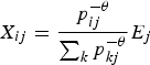
The consumption side of the prototypical trade model, which gives rise to the gravity equation in (3), satisfies property 2. The production side, which implies the proportionality in (5), satisfies property 3 with $A_{i} L_{i} = {\bar{c}}_{i}$ . Properties 1, 4, and 5 are stated directly in the description of this model, specifically in (1), (2), and (4). Finally, property 6 is a normalization that does not conflict with the prototypical model because an equilibrium in that model determines the value of relative prices but not the price level, which is a free parameter. This additional degree of freedom is removed by the normalization.

Allen, Arkolakis, and Takahashi (2020) show that various other models also satisfy the six properties of the universal gravity framework, among them the models by Arm- ington (1969), Anderson (1979), Anderson and van Wincoop (2003), Krugman (1980), Eaton and Kortum (2002), Melitz (2003), di Giovanni and Levchenko (2013), Allen and Arkolakis (2014), Redding (2016), and Redding and Sturm (2008).

2.3 Comparative statics

Allen, Arkolakis, and Takahashi (2020) show that the response of prices to a change in the trade cost matrix can be obtained by solving a system of equations that is the same for all models in the universal gravity framework that have the same trade elasticity θ and supply elasticity ψ. In this section, we present a slightly more general version of the system of equations that allows for unbalanced trade, changes in trade deficits, and changes in supply shifters.

We use the “hat algebra” notation introduced by Dekle, Eaton, and Kortum (2008). For each variable, its hat version is defined as the ratio of the value of the variable in a counterfactual equilibrium relative to the value in a baseline equilibrium; if x is the value in the baseline equilibrium and x′ is the value in the counterfactual equilibrium, then $\hat{x} \equiv x^{'} / x$ .

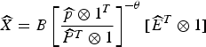
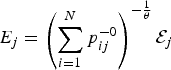
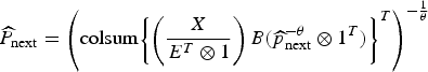
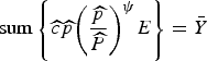
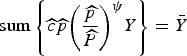
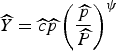
The comparative statics exercise we consider allows for a change in the matrix of bilateral trade costs with elements ${\hat{τ}}_{i j} \equiv τ_{i j}^{^{'}} / τ_{i j}$ and also for changes in the vectors of parameters ${\hat{ξ}}_{i} \equiv ξ_{i}^{^{'}} / ξ_{i}$ , which affect trade deficits, and in the supply shifters ${\hat{c}}_{i} \equiv {\bar{c}}_{i}^{^{'}} / {\bar{c}}_{i}$ . The bilateral trade flow matrix X = [X_ij]_N _× _N is assumed to be known. Income and expenditure by location and the global value of trade are obtained from the bilateral trade flow matrix as $Y_{i} \equiv \sum_{j} X_{i j}$ , $E_{i} \equiv \sum_{j} X_{i j}$ , and $\bar{Y} \equiv \sum_{i} \sum_{j} X_{i j}$ .

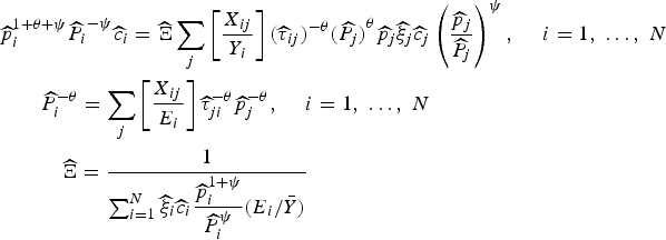
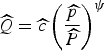
As shown in the online appendix, if prices and quantities in the baseline and the counterfactual are part of an equilibrium that satisfies the six properties of the universal gravity framework, then the changes in price vectors $({\hat{p}}_{i})_{N \times 1}$ and $({\hat{P}}_{i})_{N \times 1}$ must solve the following system of 2N + 1 nonlinear equations:

\begin{aligned} {\hat{p}}_{i}^{1 + θ + ψ} {\hat{P_{i}}}^{- ψ} {\hat{c}}_{i} = \hat{Ξ} \sum_{j} [\frac{X_{i j}}{Y_{i}}] {({\hat{τ}}_{i j})}^{- θ} {({\hat{P}}_{j})}^{θ} {\hat{p}}_{j} {\hat{ξ}}_{j} {\hat{c}}_{j} {(\frac{{\hat{p}}_{j}}{{\hat{P}}_{j}})}^{ψ}, i = 1, \dots, N \\ {\hat{P}}_{i}^{- θ} = \sum_{j} [\frac{X_{i j}}{E_{i}}] {\hat{τ}}_{j i}^{- θ} {\hat{p}}_{j}^{- θ}, i = 1, \dots, N \\ \hat{Ξ} = \frac{1}{\sum_{i = 1}^{N} {\hat{ξ}}_{i} {\hat{c}}_{i} \frac{{\hat{p}}_{i}^{1 + ψ}}{{\hat{P}}_{i}^{ψ}} (E_{i} / \bar{Y})} \end{aligned}

Once this system is solved, other quantities can be derived from the resulting price vectors. For example, in the case of the prototypical trade model, because of the proportionality relationships shown earlier, the comparative statics for output and income can be obtained immediately as

\begin{aligned} {\hat{Q}}_{i} = \frac{{\hat{w}}_{i}}{{\hat{p}}_{i}} = {\hat{c}}_{i} {(\frac{{\hat{p}}_{i}}{{\hat{P}}_{i}})}^{ψ} \\ {\hat{Y}}_{i} = {\hat{p}}_{i} {\hat{Q}}_{i} = {\hat{c}}_{i} \frac{{\hat{p}}_{i}^{1 + ψ}}{{\hat{P}}_{i}^{ψ}} \end{aligned}

where

{\hat{c}}_{i} = {\hat{A}}_{i} {\hat{L}}_{i}

and the comparative of statics for welfare are given by

{\hat{W}}_{i} = \hat{Ξ} {\hat{ξ}}_{i} \frac{{\hat{w}}_{i}}{{\hat{P}}_{i}} = \hat{Ξ} {\hat{ξ}}_{i} \frac{{\hat{c}}_{i}}{{\hat{L}}_{i}} {(\frac{{\hat{p}}_{i}}{{\hat{P}}_{i}})}^{1 + ψ}

Comparative statics for expenditure are determined by

{\hat{E}}_{i} = \hat{Ξ} {\hat{ξ}}_{i} {\hat{Y}}_{i}

and the change in bilateral trade flows can be calculated as

{\hat{X}}_{i j} = {\hat{τ}}_{i j}^{- θ} {\hat{p}}_{i}^{- θ} {\hat{P}}_{j}^{θ} {\hat{E}}_{j}

The comparative statics derived for welfare and output are specific to the prototypical model presented in this article. Other models may yield different results, especially for welfare. However, the comparative statics for some of the variables are quite general in that they are common to all models in the universal gravity framework. This holds for prices and, conditional on the price normalization, also for the value bilateral trade flows, expenditure, and income.

2.4 Algorithm to solve for prices (universal option)

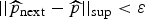
We first present the most general version of the algorithm, which is used when the ge_gravity2 command is called with the universal option. The algorithm used to solve for prices is a fixed-point algorithm in the style of Alvarez and Lucas (2007). Its structure and implementation are very similar to the algorithm used by Zylkin (2019) in the ge_gravity command. There are two major differences. The first difference is that the algorithm solves for the vector of output prices instead of wages because the universal gravity framework is agnostic about which factors of production are involved in the production process. In fact, there may be models within the universal gravity framework for which there is no properly defined wage rate. The second difference is that the algorithm has more inputs than the algorithm in ge_gravity because it accounts for exogenous changes in supply shifters and arbitrary exogenous adjustments to trade deficits in addition to the value of the supply elasticity.

Notation. In the description of the algorithm, we use the Mata functions rowsum(), colsum(), and sum(), which are defined as follows (this is how they work in Mata). rowsum() sums the elements of a matrix along each row and returns a column vector. colsum() sums the elements of a matrix along each column and returns a row vector. sum() sums all elements of a vector or matrix and returns a scalar. The symbol $\otimes$ represents the Kronecker product. All other operations, such as multiplication, division, and exponentiation, are performed element by element. All vectors are N × 1 column vectors, and all matrices are N × N square matrices, where N is the number of locations. We use the notation 1 for a column vector of size N × 1 filled with ones. The operation of transposing a vector or matrix is denoted by the superscript T.

Inputs. The required inputs to the algorithm consist of a matrix of bilateral trade flows, which we will call X, a matrix B that encodes the change in bilateral trade costs, and two scalars, one for the trade elasticity and one for the supply elasticity.

The matrix X is a square matrix containing bilateral trade flows from locations in the rows to locations in the columns. The order of the locations that appear in the rows and columns must match, and there must be no missing values (although there can be zeros). This matrix is created from a user-supplied variable containing bilateral trade flows.

The second key input is a matrix that encodes the partial equilibrium effects of changes in trade costs. We will call this matrix B. It has the same dimensions as X, and the element in row i and column j codifies how trade costs would affect trade flows from location i to location j in partial equilibrium. In terms of the notation used in the model, the element in row i and column j of B corresponds to ${\hat{τ}}_{i j}^{- θ}$ .³

The remaining two required inputs are the trade elasticity θ and the supply elasticity ψ. In addition to the required inputs, there are two additional input vectors that can be optionally provided to the algorithm: the vector $\hat{ξ}$ , which governs the discrepancy between expenditures and revenues and ultimately trade deficits, and the vector $\hat{c}$ , which governs the relative changes in the supply shifters. If these optional inputs are not provided, then they are set to be column vectors of size N × 1 filled with ones.

Algorithm 1 (universal option). The algorithm solves the system of equations for prices by iterating until the vector of output prices converges. The steps involved in the iteration are as follows:

Step 0. Choose a tolerance level for convergence ε > 0. Compute the vectors E = colsum(X) ^T and Y = rowsum(X) and the scalar $\bar{Y} = sum (X)$ . Initialize the vectors $\hat{p} = 1$ and $\hat{P} = 1$ .

Step 1. Compute the scalar $\hat{Ξ}$ :

\hat{Ξ} = \bar{Y} / sum {\hat{ξ} \hat{c} \hat{p} {(\frac{\hat{p}}{\hat{P}})}^{ψ} E}

Step 2. Update the vector $\hat{p}$ :

{\hat{p}}_{next} = {(\hat{Ξ} [\frac{{\hat{P}}^{ψ}}{\hat{c}}] rowsum [(\frac{X}{Y \otimes 1^{T}}) B {{(\hat{ξ} \hat{c} {\hat{P}}^{θ - ψ} {\hat{p}}^{1 + ψ})}^{T} \otimes 1}])}^{\frac{1}{1 + θ + ψ}}

Step 3. Update the vector $\hat{P}$ :

{\hat{P}}_{next} = {(colsum {(\frac{X}{E^{T} \otimes 1}) B ({\hat{p}}_{next}^{- θ} \otimes 1^{T})}^{T})}^{- \frac{1}{θ}}

Step 4. Check convergence:

| | {\hat{p}}_{next} - \hat{p} | |_{sup} < ε

If convergence was achieved, then stop. If not, then set

\hat{p} - {\hat{p}}_{next}

and

\hat{P} - {\hat{P}}_{next}

and return to step 1.

Outputs. Once the algorithm has converged, the vector of output prices $\hat{p}$ , the vector of price indices $\hat{P}$ , and the scalar $\hat{Ξ}$ are known.

2.5 Algorithm to solve for prices with constant trade deficits (default option)

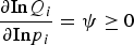
The algorithm just described is the one used when the user runs the ge_gravity2 command with the universal option. For many applications, it may be more convenient to assume that trade deficits are constant. The case with constant trade deficits is the default option of the existing ge_gravity command, and we make it the default of the newer ge_gravity2 command as well, meaning that the algorithm for constant trade deficits is used unless the user chooses either the universal or the multiplicative option. Constant deficits can be implemented as a special case in the universal gravity framework by making the change in ξ _i parameters endogenous.

To derive the algorithm, we start from (4):

Ξ ξ_{i} p_{i} Q_{i} = E_{i} = D_{i} + p_{i} Q_{i}

The equality on the left is given as a definition in property 5 of the universal gravity framework, and the equality on the right is the usual definition of trade deficits.

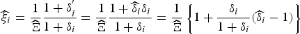
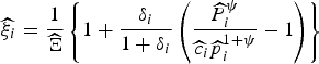
Solving this equation for ξ _i leads to

ξ_{i} = \frac{1}{Ξ} (1 + \frac{D_{i}}{p_{i} Q_{i}}) = \frac{1}{Ξ} (1 + δ_{i})

where we have defined δ_i as the ratio of the trade deficit to income:

δ_{i} \equiv \frac{D_{i}}{p_{i} Q_{i}}

The change in the endogenous variable ${\hat{ξ}}_{i}$ is then determined by

{\hat{ξ}}_{i} = \frac{1}{\hat{Ξ}} \frac{1 + δ_{i}^{^{'}}}{1 + δ_{i}} = \frac{1}{\hat{Ξ}} \frac{1 + {\hat{δ}}_{i} δ_{i}}{1 + δ_{i}} = \frac{1}{\hat{Ξ}} {1 + \frac{δ_{i}}{1 + δ_{i}} ({\hat{δ}}_{i} - 1)}

The last step is to derive an expression for

{\hat{δ}}_{i}

in terms of price changes and supply shifters. Using the condition that deficits remain constant, that is,

D_{i}^{^{'}} = D_{i}

, this can be done as follows:

{\hat{δ}}_{i} = \frac{D_{i}^{^{'}} / (p_{i}^{^{'}} Q_{i}^{^{'}})}{D_{i} / (p_{i} Q_{i})} = \frac{D_{i} / (p_{i}^{^{'}} Q_{i}^{^{'}})}{D_{i} / (p_{i} Q_{i})} = \frac{1}{{\hat{p}}_{i} {\hat{Q}}_{i}} = \frac{1}{{\hat{Y}}_{i}} = \frac{{\hat{P}}_{i}^{ψ}}{{\hat{c}}_{i} {\hat{p}}_{i}^{1 + ψ}}

Finally, putting the previous results together, the endogenous change of

{\hat{ξ}}_{i}

required to maintain trade deficits constant is

{\hat{ξ}}_{i} = \frac{1}{\hat{Ξ}} {1 + \frac{δ_{i}}{1 + δ_{i}} (\frac{{\hat{P}}_{i}^{ψ}}{{\hat{c}}_{i} {\hat{p}}_{i}^{1 + ψ}} - 1)}

The modifications with respect to the previous algorithm consist of initializing $\hat{Ξ}$ to one and adding an extra step just before step 1 that calculates the endogenous change in ${\hat{ξ}}_{i}$ parameters that keeps trade deficits constant.

Algorithm 2 (default option).

Step 0. Choose a tolerance level for convergence ε > 0. Compute the vectors E = colsum(X) ^T , Y = rowsum(X), and the scalar $\bar{Y} = sum (X)$ . Compute the vector δ = (E — Y)/Y. Initialize the vectors $\hat{p} = 1$ and $\hat{P} = 1$ . Initialize the scalar $\hat{Ξ} = 1$ .

Step 0.5. Compute the vector $\hat{ξ}$ :

\hat{ξ} = \frac{1}{\hat{Ξ}} {1 + \frac{δ}{1 + δ} (\frac{{\hat{P}}^{ψ}}{\hat{c} {\hat{p}}^{1 + ψ}} - 1)}

Step 1. Compute the scalar $\hat{Ξ}$ :

\hat{Ξ} = \bar{Y} / sum {\hat{ξ} \hat{c} \hat{p} {(\frac{\hat{p}}{\hat{P}})}^{ψ} E}

Step 2. Update the vector $\hat{p}$ :

{\hat{p}}_{next} = {(\hat{Ξ} [\frac{{\hat{P}}^{ψ}}{\hat{c}}] rowsum [(\frac{X}{Y \otimes 1^{T}}) B {{(\hat{ξ} \hat{c} {\hat{P}}^{θ - ψ} {\hat{p}}^{1 + ψ})}^{T} \otimes 1}])}^{\frac{1}{1 + θ + ψ}}

Step 3. Update the vector $\hat{P}$ :

{\hat{P}}_{next} = {[colsum {(\frac{X}{E^{T} \otimes 1}) B ({\hat{p}}_{next}^{- θ} \otimes 1^{T})}^{T}]}^{- \frac{1}{θ}}

Step 4. Check convergence:

| | {\hat{p}}_{next} - \hat{p} | |_{sup} < ε

If convergence was achieved, then stop. If not, then set

\hat{p} = {\hat{p}}_{next}

and

\hat{P} = {\hat{P}}_{next}

next and return to step 0.5.

Outputs. Once the algorithm has converged, the vector of output prices $\hat{p}$ , the vector of price indices $\hat{P}$ , and the scalar $\hat{Ξ}$ are known.

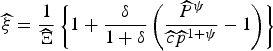
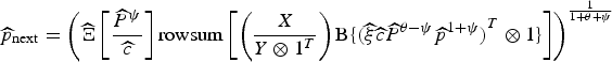
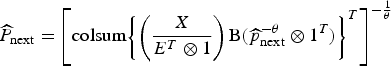
Running the ge_gravity2 command with a supply elasticity of 0 and the default options will replicate the results of ge_gravity with the default options.

2.6 Algorithm to solve for prices with multiplicative trade deficits (multiplicative option)

The ge_gravity command has a multiplicative option in which trade deficits are assumed to evolve at all locations in a way that satisfies the equation

{\hat{E}}_{i} = \frac{Y_{i}^{^{'}} + D_{i}^{^{'}}}{Y_{i} + D_{i}} = {\hat{Y}}_{i}

In ge_gravity2, we also implement the multiplicative option to make the command backward compatible with ge_gravity. For the change in expenditure and income to coincide at all locations, it is necessary to set ${\hat{ξ}}_{i} = 1$ for all i and $\hat{Ξ} = 1$ . This means that step 1 can no longer be used in the algorithm. However, because there is no need to solve for $\hat{Ξ}$ in this case, it is possible to replace step 1 (which relies on properties 5 and 6) with the price normalization of property 6 directly. From this property applied to the baseline and counterfactual economy we have that

\bar{Y} = \sum_{i = 1}^{N} Y_{i}^{^{'}} = \sum_{i = 1}^{N} {\hat{Y}}_{i} Y_{i} = \sum_{i = 1}^{N} {\hat{c}}_{i} \frac{{\hat{p}}_{i}^{1 + ψ}}{{\hat{P}}_{i}^{ψ}} Y_{i}

The right-hand side of this equation is homogeneous of degree one in price changes, and we can use this equation to normalize prices. We add a new step in the algorithm right after step 3 that does this.

Algorithm 3 (multiplicative option).

Step 0. Choose a tolerance level for convergence ε > 0. Compute the vectors E = colsum(X) ^T , Y = rowsum(X), and the scalar $\bar{Y} = sum (X)$ . Initialize the vectors $\hat{p} = 1$ and $\hat{P} = 1$ . Set the vector $\hat{ξ} = 1$ . Set the scalar $\hat{Ξ} = 1$ .

Step 1. (omitted).

Step 2. Update the vector $\hat{p}$ :

{\hat{p}}_{next} = {(\hat{Ξ} [\frac{{\hat{P}}^{ψ}}{\hat{c}}] rowsum [(\frac{X}{Y \otimes 1^{T}}) B {{(\hat{ξ} \hat{c} {\hat{P}}^{θ - ψ} {\hat{p}}^{1 + ψ})}^{T} \otimes 1}])}^{\frac{1}{1 + θ + ψ}}

Step 3. Update the vector $\hat{P}$ :

{\hat{P}}_{next} = {[colsum {(\frac{X}{E^{T} \otimes 1}) B ({\hat{p}}_{next}^{- θ} \otimes 1^{T})}^{T}]}^{- \frac{1}{θ}}

Step 3.5. Compute the scalar ρ (excess world income) asand normalize the price vectors $\hat{p}$ and $ρ = sum {\hat{c} \hat{p} {(\frac{\hat{p}}{\hat{P}})}^{ψ} Y} / \bar{Y}$ $\hat{P}$ by dividing them by ρ.

Step 4. Check convergence:

| | {\hat{p}}_{next} - \hat{p} | |_{sup} < ε

If convergence was achieved, then stop. If not, then set

\hat{p} = {\hat{p}}_{next}

and

\hat{P} = {\hat{P}}_{next}

and return to step 2.

Outputs. Once the algorithm has converged, the vector of normalized output prices $\hat{p}$ and the vector of normalized price indices $\hat{P}$ are known. The scalar $\hat{Ξ}$ always equals 1 in this case.

Running the ge_gravity2 command with the multiplicative option and a supply elasticity of 0 will replicate the results obtained by ge_gravity with the option multiplicative.

Comparison with the universal option. The results that are obtained with the multiplicative option will generally not match those obtained with the universal option, even when $\hat{ξ} = 1$ , although they will be close if the trade deficits are not too large. The difference between these two options is that the change in nominal quantities is determined in a different way. Note that step 1 of the universal algorithm with $\hat{Ξ} = 1$ and $\hat{ξ} = 1$ results in

sum {\hat{c} \hat{p} {(\frac{\hat{p}}{\hat{P}})}^{ψ} E} = \bar{Y}

whereas the normalization in the multiplicative algorithm implies that prices satisfy

sum {\hat{c} \hat{p} {(\frac{\hat{p}}{\hat{P}})}^{ψ} Y} = \bar{Y}

These two normalizations are equivalent if expenditures coincide with incomes, meaning that trade deficits are 0, but are generally different when they are not.

2.7 Remaining calculations

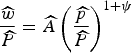
Once price changes have been obtained, other variables follow in order. We maintain the convention that all operations except the Kronecker product are performed element by element. The change in income is obtained directly from the price changes as

\hat{Y} = \hat{c} \hat{p} {(\frac{\hat{p}}{\hat{P}})}^{ψ}

The change in expenditure then follows as

\hat{E} = \hat{Ξ} \hat{ξ} \hat{Y}

Changes in bilateral trade flows are obtained as

\hat{X} = B {[\frac{\hat{p} \otimes 1^{T}}{{\hat{P}}^{T} \otimes 1}]}^{- θ} [{\hat{E}}^{T} \otimes 1]

For the prototypical trade model, the change in real prices also translates directly into changes in real output, which is obtained as

\hat{Q} = \hat{c} {(\frac{\hat{p}}{\hat{P}})}^{ψ}

The computation for the change in welfare depends on whether the change in supply shifters is generated by changes in productivity or the labor force. For the prototypical trade model, the vector

\hat{c}

is the product of

\hat{A}

and

\hat{L}

, and the change in welfare can be expressed as

\hat{W} = \hat{Ξ} \hat{ξ} \frac{\hat{c}}{\hat{L}} {(\frac{\hat{p}}{\hat{P}})}^{1 + ψ} = \hat{Ξ} \hat{ξ} \hat{A} {(\frac{\hat{p}}{\hat{P}})}^{1 + ψ}

The syntax of the ge_gravity2 command includes options that allow the user to specify

\hat{A}

and

\hat{L}

or to specify

\hat{c}

. Welfare is calculated only if the user specifies

\hat{A}

vor

\hat{L}

, or both at the same time, but not if the user specifies

\hat{c}

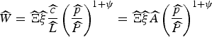
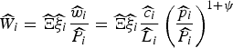
The changes of real and nominal wages in the prototypical trade model also depend on the distinction between $\hat{A}$ and $\hat{L}$ . They are calculated as

\frac{\hat{w}}{\hat{P}} = \hat{A} {(\frac{\hat{p}}{\hat{P}})}^{1 + ψ}

and

\hat{w} = \hat{P} \hat{A} {(\frac{\hat{p}}{\hat{P}})}^{1 + ψ} = \hat{A} \frac{{\hat{p}}^{1 + ψ}}{{\hat{P}}^{ψ}}

2.7 Reporting comparative statics for the prototypical trade model

The normalization in property 6 determines the scale of nominal quantities in all universal gravity models. Because the prototypical trade model determines only real variables, we said earlier that property 6 does not conflict with the model. However, there is a subtle point that needs to be clarified. The use of normalization in property 6 is harmless for equilibrium objects in the baseline economy and in the counterfactual economy when considered in isolation. However, when doing comparative statics, using the same normalization in both models introduces an additional assumption. In this case, the assumption is that global nominal income is the same in the baseline and the counter- factual. This assumption may not be consistent with the intended use of the model. Researchers should therefore be cautious when reporting comparative static calculations for nominal quantities. Thus, the default results table generated by the command shows growth rates only for real variables.

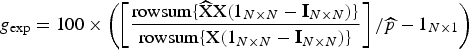
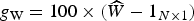
The default calculation reports the vector relative changes of real (nondomestic) exports for all locations, which is calculated as

g_{\exp} = 100 \times ([\frac{rowsum {\hat{X} X (1_{N \times N} - I_{N \times N})}}{rowsum {X (1_{N \times N} - I_{N \times N})}}] / \hat{p} - 1_{N \times 1})

Here 1 _N _× _N denotes a square matrix of size N filled with 1 s, and 1 _N _× ₁ denotes a N × 1 unitary vector. We use the notation I _N _× _N to refer to the identity matrix of size N. We continue using the convention that all operations are performed element by element. Notice that multiplying a matrix by the term (1 _N _× _N - I _N _× _N ) is equivalent to setting its diagonal elements to 0. We do this to exclude domestic trade from the calculation. The relative change in exports is real (as opposed to nominal) because the nominal change of exports is deflated by the change in export prices

\hat{p}

in the equation above.

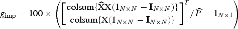
Similarly, the vector of real relative changes of imports is calculated as

g_{imp} = 100 \times ({[\frac{colsum {\hat{X} X (1_{N \times N} - I_{N \times N})}}{colsum {X (1_{N \times N} - I_{N \times N})}}]}^{T} / \hat{P} - 1_{N \times 1})

This expression is very similar to the expression for exports. The main differences are that matrices are summed over columns (that is, across rows for each column) to obtain imports instead of exports and that the nominal change is deflated by the change in the consumer price index

\hat{P}

, instead of the change in export prices

\hat{p}

The relative change in total trade is obtained as the weighted average of the relative changes of exports and imports, where the weights are given by exports and imports in the baseline economy. The change in domestic trade is calculated from the diagonal elements of the bilateral trade matrix $\hat{X}$ as follows:

g_{dom} = 100 \times {diagonal (\hat{X}) / \hat{P} - 1_{N \times 1}}

This implies that domestic trade is also deflated by the consumer price index

\hat{P}

Finally, the relative change of real output and welfare is computed as

g_{Q} = 100 \times (\hat{Q} - 1_{N \times 1})

and

g_{W} = 100 \times (\hat{W} - 1_{N \times 1})

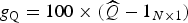
All of these relative changes are expressed in percentage points. They are to be interpreted as the impact of moving from the baseline situation to the counterfactual situation, not as growth rates of variables over time.

2.9 The matrix of partial equilibrium effects

The matrix B is a key input to the three algorithms used to solve for price changes. It encodes the partial equilibrium effects of changes in bilateral trade costs. Specifically, each element B _ij corresponds to the term ${\hat{τ}}_{i j}^{- θ}$ , where ${\hat{τ}}_{i j}$ is the change in iceberg trade costs faced by trade flows exported by i to importer j and θ is the trade elasticity.

Users of the ge_gravity2 command do not construct the matrix B explicitly. Instead, they provide the information on changes in bilateral trade costs using the variable called partial in the syntax of the command. This variable contains the partial equilibrium effect of changes in trade policies.

Partial equilibrium effects are frequently obtained from a prior gravity estimation that imposes

E (X_{i j t} | observables) = \exp {\ln (τ_{i j t}^{- θ}) + other terms}

where t denotes time and the other terms typically include exporter-time and importertime fixed effects and, sometimes, pair fixed effects. Such an equation can be derived from the theoretical gravity equation for bilateral trade flows given in section 2, assuming that the theory applies to all dates t. The iceberg cost τ _ijt is usually specified parametrically. For example, a researcher might assume that

\ln (τ_{i j t}^{- θ}) = β z_{i j t} + other variables

where z_ijt is a dummy variable that indicates whether trade between exporter i and importer j was subject to a free trade agreement in year t.

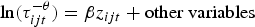
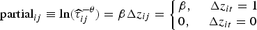
The parameter β has the interpretation of a partial equilibrium semielasticity; it measures the relative change in trade flows associated with switching the dummy variable z_ijt from 0 to 1, holding all other variables constant. The fixed effects that are usually included in the regression absorb any general equilibrium effects (for example, changes in country-specific output prices ${\hat{p}}_{i}$ price indices ${\hat{P}}_{i}$ and expenditure ${\hat{E}}_{i}$ ).

The change from a situation without a trade agreement to one with a trade agreement implies the following change in bilateral trade costs:

{partial}_{i j} \equiv \ln ({\hat{τ}}_{i j}^{- θ}) = β Δ z_{i j} = {\begin{matrix} β, Δ z_{i t} = 1 \\ 0, Δ z_{i t} = 0 \end{matrix}

The ge_gravity2 command constructs B internally from the user-provided variable partial _ij , applying an exponential transformation to the partial equilibrium effects:

B_{i j} = {\hat{τ}}_{i j}^{- θ} = \exp ({partial}_{i j}) = {\begin{matrix} \exp (β), Δ z_{i t} = 1 \\ 1, Δ z_{i t} = 0 \end{matrix}

This behavior replicates the behavior of the prior command ge_gravity. The examples in section 4 show how to construct the variable that contains the partial equilibrium effects for various different exercises.

Remark. The matrix B is useful to simulate a counterfactual that involves a change in bilateral trade costs. This includes, for instance, trade policy simulations, such as the formation of a free trade agreement, or the removal of nontariff trade barriers. In contrast, when the counterfactual exercise involves only changes in productivity, in labor supply, or in trade deficits, the partial equilibrium effects of trade costs are 0, and the matrix B is filled with 1 s.

3 The ge_gravity2 command

3.1 Syntax

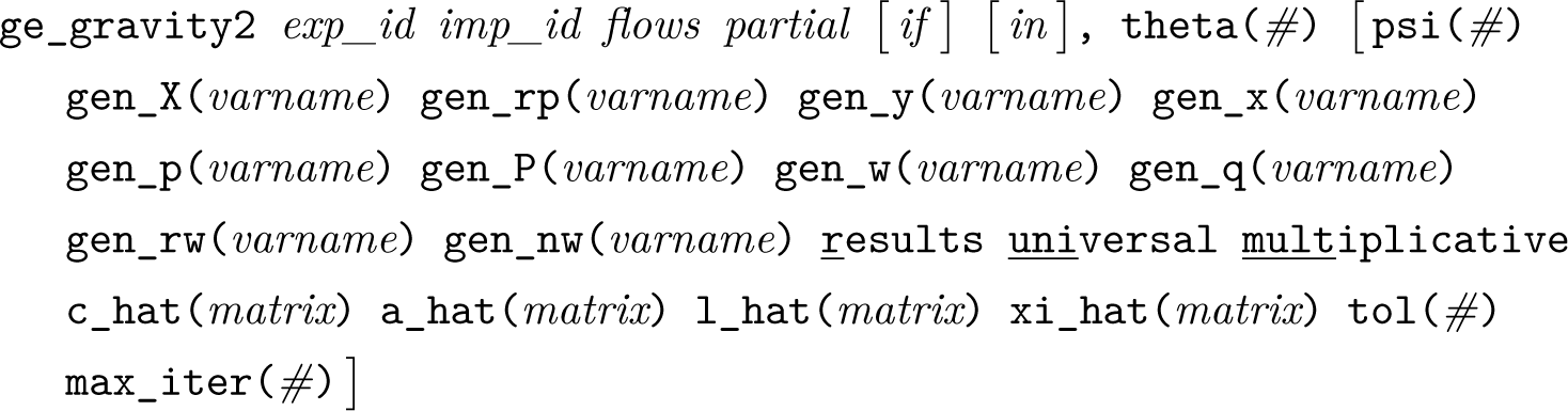
3.2 Required variables

exp_id specifies the variable that identifies the location of origin, for example, ISO codes or names of countries. This variable can be a string variable or numeric. It cannot contain missing values.

imp_id specifies the variable that identifies the location of destination, for example, ISO codes or names of countries. This variable can be a string variable or numeric. It cannot contain missing values.

flows contains bilateral trade flows. This variable contains the flow from the location identified as exp_id to the location identified as imp_id . This variable cannot contain missing values but can contain zeros.

partial contains the “partial” estimate of the effect, typically obtained as a coefficient from a prior gravity estimation. This variable cannot contain missing values.

3.3 Options

3.3.1 Elasticities

theta(#) sets the trade elasticity, which must be strictly positive. theta() is required.

psi(#) sets the aggregate supply elasticity, which must be nonnegative. The default is psi(0). With a supply elasticity of 0, the command solves essentially the same model as ge_gravity.

3.3.2 New variables (universal gravity)

gen_X(varname) generates counterfactual trade flows (X′ in the model) and places the result in a new variable called varname or overwrites this variable if it already exists.

gen_rp(varname) generates the change in real prices ( $\hat{p} / \hat{P}$ in the model) and places the result in a new variable called varname or overwrites this variable if it already exists.

gen_y(varname) generates the change in income ( $\hat{Y}$ in the model) and places the result in a new variable called varname or overwrites this variable if it already exists.

gen_x(varname) generates the change in trade flows ( $\hat{X}$ in the model) and places the result in a new variable called varname or overwrites this variable if it already exists.

gen_p(varname) generates the change in output prices ( $\hat{p}$ in the model) and places the result in a new variable called varname or overwrites this variable if it already exists.

gen_P(varname) generates the change in price indices ( $\hat{P}$ in the model) and places the result in a new variable called varname or overwrites this variable if it already exists.

3.3.3 New variables (prototypical model)

gen_w(varname) generates the change in welfare ( $\hat{W}$ in the model) and places the result in a new variable called varname or overwrites this variable if it already exists.

gen_q(varname) generates the change in real output ( $\hat{Q}$ in the model) and places the result in a new variable called varname or overwrites this variable if it already exists.

gen_rw(varname) generates the change in real wages ( $\hat{w} / \hat{P}$ in the model) and places the result in a new variable called varname or overwrites this variable if it already exists.

gen_nw(varname) generates the change in nominal wages ( $\hat{w}$ in the model) and places the result in a new variable called varname or overwrites this variable if it already exists.

3.3.4 Other options

results prints a table with percent changes for exports, imports, total trade, domestic trade, real output, and welfare.

universal solves the model with universal trade deficits and allows the user to set the option xi_hat().

multiplicative solves the model for trade deficits that imply $\hat{E} = \hat{Y}$ (for backward compatibility with the multiplicative option of the ge_gravity command).

c_hat(matrix) changes supply shifters ( $\hat{c}$ in the model). Welfare will not be calculated if this option is used. This option may not be combined with the option a_hat() or l_hat(). The default behavior is that all elements of c_hat() are set to 1.

a_hat(matrix) changes productivity ( $\hat{A}$ in the prototypical trade model). This option may not be combined with the option c_hat(). The default behavior is that all elements of a_hat() are set to 1.

l_hat(matrix) changes the labor force ( $\hat{L}$ in the prototypical trade model). This option may not be combined with the option c_hat(). The default behavior is that all elements of l_hat() are set to 1.

xi_hat(matrix) changes trade deficits ( $\hat{ξ}$ in the model). This option must be used in combination with the universal option. If the universal option is selected and the xi_hat option is not used, then the command defaults to setting all elements of xi_hat() to 1.

tol(#) sets the tolerance level to verify convergence of the vector of output price changes. The tolerance level must be a strictly positive real number. The default is tol(1e-12).

max_iter(#) sets the maximum number of iterations to solve for the vector of output price changes. The maximum number of iterations must be a positive integer. The default is max_iter(1000000).

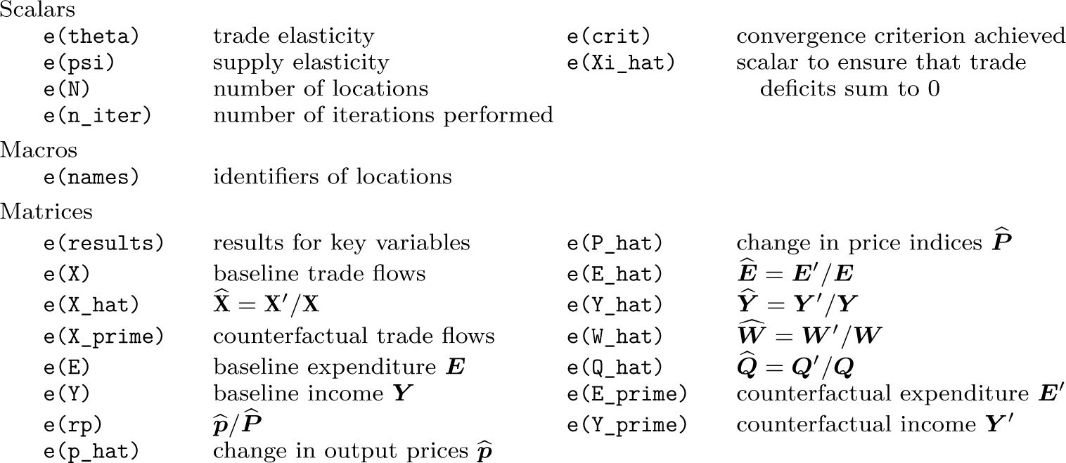
3.4 Stored results

ge_gravity2 stores the following in e() :

4 Examples

All three examples use ge_gravity2_example_data.dta, which is available with the article files. In this dataset, the string variable iso_o identifies the country of origin, and the string variable iso_d identifies the country of destination. The variable flow contains bilateral trade flows from iso_o to iso_d, and the variable year identifies years (in 10-year increments).

4.1 A simulation of the ex ante effect of a trade agreement

In a first example, we simulate the effect of a free trade agreement. Suppose that we want to compute the expected effects of the North American Free Trade Agreement, a trade agreement signed by Canada, Mexico, and the United States that entered into force in 1994. Also, suppose that we expect the partial equilibrium effect of this trade agreement to be 0.5, meaning that countries that are part of this trade agreement are expected to increase their trade flows with other members by exp(0.5) ‒ 1 ≈ 65% if nothing else changes. The general equilibrium impact of this agreement can then be computed issuing the following commands in Stata:

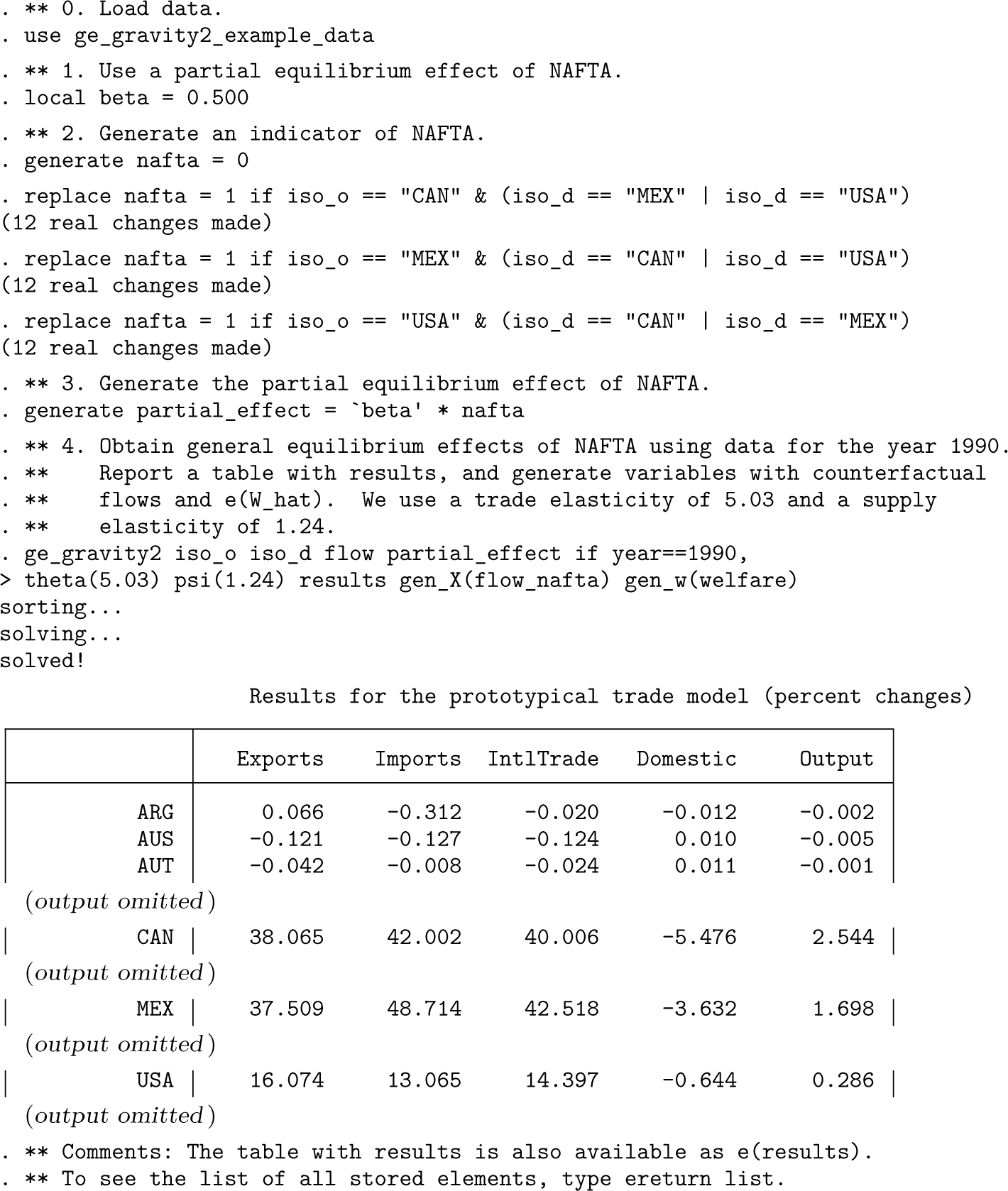
After running this code, the command will print out a table that exhibits the change in trade flows, output, and welfare for all countries in the sample. We show only an excerpt from the table showing the first three lines and the countries involved in the trade agreement.

Because we specified the option gen_w(welfare), the command will also have generated a new variable called welfare, which contains the comparative statics for welfare $\hat{W_{i}} = W_{i}^{^{'}} / W_{i}$ for every country i (i in this case refers to the country that is listed in the variable iso_o). This new variable will have nonmissing values only in the year 1990 because the command was issued specifying the condition if year==1990. Because the trade model is static, a researcher will want to use data only from a particular year, as we did in this example, except in rare cases.

In this example, we have used a trade elasticity of 5.03, taken from the handbook chapter by Head and Mayer (2014). Values of 4 or 5 are common in policy studies quantifying the effects of free trade agreements. There is less consensus on the value of supply elasticity. Alvarez and Lucas (2007) suggest using a supply elasticity of 1, and Eaton and Kortum (2002) suggest a value of 3.76. In this example, we have taken the value of 1.24 from a calculation by Campos et al. (2023), who chose the supply elasticity as the midpoint of the supply elasticities implied by the 10th and 90th percentiles of the distribution of the range of intermediate goods shares for the sample of countries in the KLEMS database, as reported by Huo, Levchenko, and Pandalai-Nayar (2025).

The command in this example was run using the default algorithm. This means that the trade deficits in the counterfactual are assumed to be the same (in nominal terms) as in the baseline economy. This is not the only option. The universal option simulates the counterfactual assuming that the ratio of expenditure to income changes in the same way for all countries. The user may want to use the universal option together with the xi_hat() option to break this homogeneity and allow expenditure to increase more in some countries than in others. Another alternative is to use the multiplicative option. In this case, expenditure and income grow at the same rate in all countries, resulting in a constant ratio of expenditure to income.

3.2 A quantification of the impact of time-varying border effects on welfare

We now turn to a more complicated example using several years of data. In this example, we use estimates of Spain’s “border thickness” by Campos, Reggio, and Timini (2023). In their article, they measure the border thickness (a measure of how difficult it is to trade internationally) of Spain during the Franco regime and compare it with the border thickness of a synthetic control for Spain that is calculated as an average of other countries. They report estimates of the welfare loss implied by Spain’s differential border thickness and interpret this welfare loss as the effect of the economic policies pursued by Spain in the postwar period until 1975.

In this example, we use the same database as before and calculate the welfare gain that Spain would have experienced if it had the border thickness of its synthetically constructed counterfactual. We do the calculation for several years. We use a trade elasticity of 4 and three different supply elasticity values: 0, 1, and 2. A trade elasticity of 4 and a supply elasticity of 0 correspond to the original simulations of Campos, Reggio, and Timini (2023).

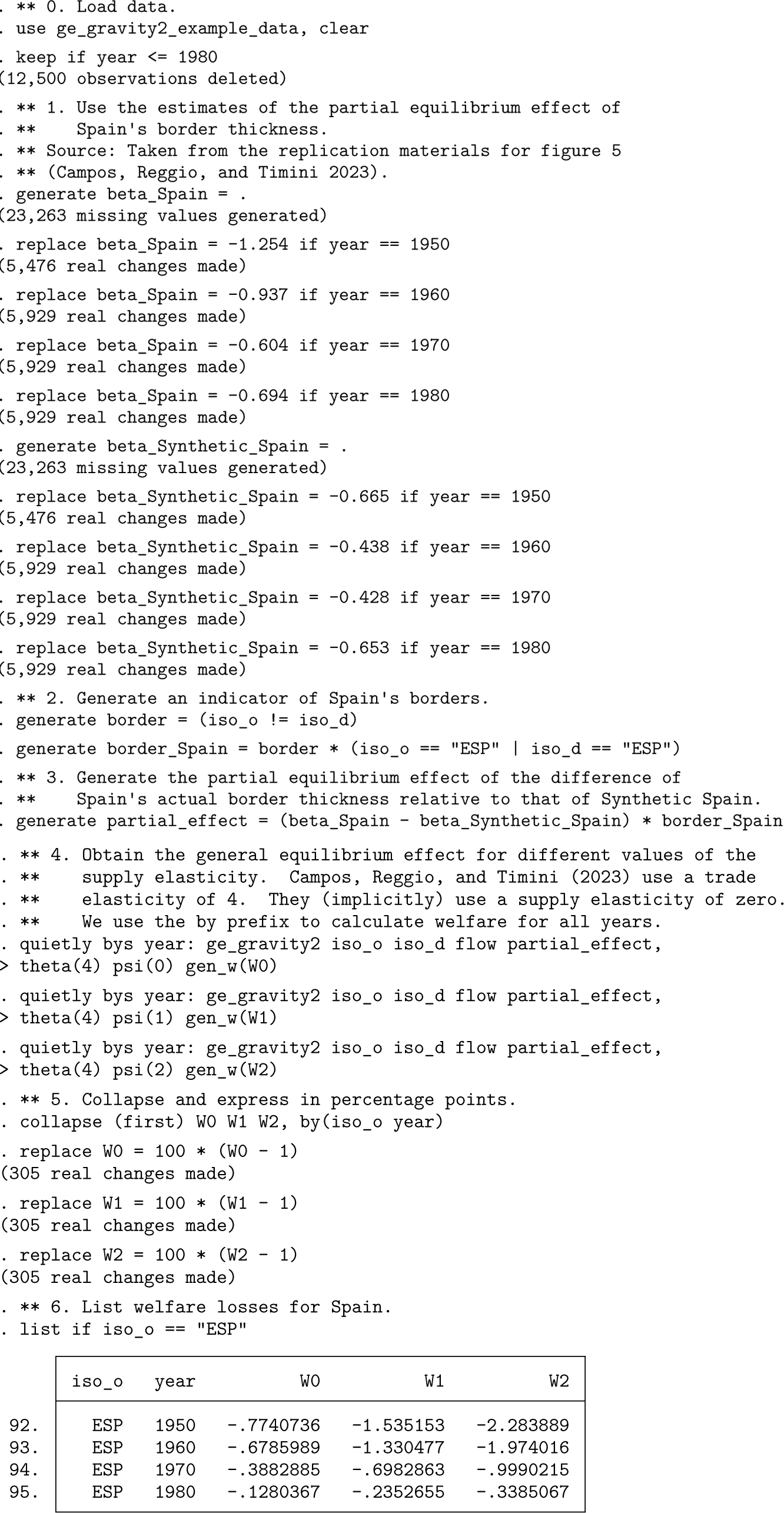
To avoid having to use a loop to simulate the model for each year, we take advantage of the fact that the ge_gravity2 command can be used with the by prefix. Although the identity and number of exporters and importers may vary across years, it is important that the data in each year are square (that is, there are the same exporters and importers and no missing values).

The results in this last listing show how the welfare calculations depend on different values of the supply elasticity. Because we used the command with the by prefix, it is not possible to generate a results table. The values for variables other than welfare can be obtained using the options that begin with the gen_ prefix.

3.3 A simulation of a change in productivity

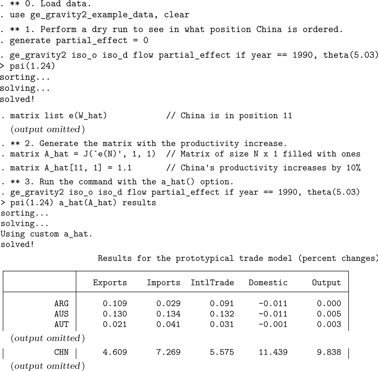
The command ge_gravity2 can also be used to run simulations in which a country’s productivity changes while its trade costs do not. In this last example, we simulate the impact that raising China’s productivity by 10% has on trade flows, output, and welfare of all countries in the world. We do this using the a_hat() option.

We show only an excerpt from the resulting table showing the first three lines and the line for China.

5 Conclusions

This article introduced the ge_gravity2 command, a substantial extension of the original ge_gravity command for structural gravity models. By enabling counterfactual simulations in a broader class of general equilibrium trade models—including those with positive aggregate supply elasticity—ge_gravity2 expands the empirical capabilities available to applied researchers. The command accommodates changes in trade frictions (including country-specific shocks, as in Freeman et al. 2025), technology, and trade imbalances, making it suitable for a wide range of academic and policy applications.

The ge_gravity2 command is designed to allow users familiar with the original ge_gravity command to transition smoothly. It aims to balance generality, tractability, and ease of use—serving both as a practical tool for policy simulation and a foundation for building more complex models.

Looking ahead, we identify three promising directions for future development. First, the current version is limited to a single-sector framework. Extending the command to incorporate sectoral heterogeneity and input-output linkages, following the structure of Caliendo and Parro (2015), would enable more granular analysis of sector-specific policies such as tariffs, nontariff measures, and industrial policies.

Second, ge_gravity2 currently implements a static model. Incorporating dynamic elements—such as capital accumulation or other intertemporal decision making—would allow researchers to study transitional dynamics and long-run effects of policy changes. While dynamic models exist, such as those by Caliendo, Dvorkin, and Parro (2019) and Kleinman, Liu, and Redding (2023), solving them is challenging. There is currently no universal template for solving them similar to the one that exists for static models. Thus, it may take time before models of this kind can be implemented easily within Stata.

Third, there is increasing academic and policy interest in understanding the interaction between trade and environmental regulation. Extending ge_gravity2 to incorporate environmental dimensions would significantly enhance its relevance for evaluating instruments such as carbon taxes, carbon border adjustments, emissions-linked trade costs, and the environmental impact of trade-induced production shifts. These features would make the command a valuable tool for analyzing the broader economic implications of environmental policy.

Supplemental Material

sj-dta-1-stj-10.1177_1536867X251398335 - Supplemental material for ge_gravity2: A command for solving universal gravity models

Supplemental material, sj-dta-1-stj-10.1177_1536867X251398335 for ge_gravity2: A command for solving universal gravity models Rodolfo G. Campos, Iliana Reggio and Jacopo Timini by in The Stata Journal

Supplemental Material

sj-pdf-2-stj-10.1177_1536867X251398335 - Supplemental material for ge_gravity2: A command for solving universal gravity models

Supplemental material, sj-pdf-2-stj-10.1177_1536867X251398335 for ge_gravity2: A command for solving universal gravity models by Rodolfo G. Campos, Iliana Reggio and Jacopo Timini in The Stata Journal

Supplemental Material

sj-txt-1-stj-10.1177_1536867X251398335 - Supplemental material for ge_gravity2: A command for solving universal gravity models

Supplemental material, sj-txt-1-stj-10.1177_1536867X251398335 for ge_gravity2: A command for solving universal gravity models by Rodolfo G. Campos, Iliana Reggio and Jacopo Timini in The Stata Journal

Footnotes

6

We have greatly benefited from comments by Tom Zylkin. The views expressed in this article are those of the authors and therefore do not necessarily reflect those of the Banco de Espana or the Eurosystem.

Iliana Reggio acknowledges funding by Ministerio de Ciencia, Innovaci0n y Univer- sidades, grant number PID2024-161540NB-I00.

7

To install the software files as they existed at the time of publication of this article, type

A more recent version of the command may be available from the Statistical Software Components Archive by typing

Notes

About the authors

Rodolfo Campos is a senior economist at Banco de España. His current research interests include macroeconomics, social insurance, and international economics.

Iliana Reggio is an associate professor of economics at Universidad Autónoma de Madrid. Her current research interests include labor economics, international economics, and applied microeconomics.

Jacopo Timini is a senior economist at Banco de España. His current research interests include international economics and economic history.

References

Allen

Arkolakis

. 2014. Trade and the topography of the spatial economy. Quarterly Journal of Economics 129: 1085–1140. 10.1093/qje/qju016.

Allen

Arkolakis

Takahashi

. 2020. Universal gravity. Journal of Political Economy 128: 393–433. 10.1086/704385.

Alvarez

Lucas

R. E.

Jr . 2007. General equilibrium analysis of the Eaton- Kortum model of international trade. Journal of Monetary Economics 54: 1726–1768. 10.1016/j.jmoneco.2006.07.006.

Anderson

J. E

. 1979. A theoretical foundation for the gravity equation. American Economic Review 69: 106–116.

Anderson

J. E.

Larch

Yotov

Y. V.

. 2018. GEPPML: General equilibrium analysis with PPML. World Economy 41: 2750–2782. 10.1111/twec.12664.

Anderson, J. E., and E. van Wincoop. 2003. Gravity with gravitas: A solution to the border puzzle. American Economic Review 93: 170–192. 10.1257/000282803321455214.

Armington

P. S

. 1969. A theory of demand for products distinguished by place of production. IMF Staff Papers 16: 159–178.

Baier

S. L.

Yotov

Y. V.

Zylkin

. 2019. On the widely differing effects of free trade agreements: Lessons from twenty years of trade integration. Journal of International Economics 116: 206–226. 10.1016/j.jinteco.2018.11.002.

Caliendo

Dvorkin

Parro

. 2019. Trade and labor market dynamics: General equilibrium analysis of the China trade shock. Econometrica 87: 741–835. 10.3982/ECTA13758.

10.

Caliendo

Parro

. 2015. Estimates of the trade and welfare effects of NAFTA. Review of Economic Studies 82: 1–44. 10.1093/restud/rdu035.

11.

Campos

R. G.

Estefania-Flores

Furceri

Timini

. 2023. Geopolitical fragmentation and trade. Journal of Comparative Economics 51: 1289–1315. 10.1016/j.jce.2023.06.008.

12.

Campos

R. G.

Reggio

Timini

. 2023. Autarky in Franco’s Spain: The costs of a closed economy. Economic History Review 76: 1259–1280. 10.1111/ehr.13243.

13.

2024. ge_gravity2: Stata module to solve a gravity model within the universal gravity class. Statistical Software Components S459317, Department of Economics, Boston College. https://ideas.repec.org/c/boc/bocode/s459317.html.

14.

Dekle

Eaton

Kortum

. 2008. Global rebalancing with gravity: Measuring the burden of adjustment. IMF Staff Papers 55: 511–540. 10.1057/imfsp.2008.17.

15.

di Giovanni, J., and A. A. Levchenko. 2013. Firm entry, trade, and welfare in Zipf’s world. Journal of International Economics 89: 283–296. 10.1016/j.jinteco.2012.08.002.

16.

Eaton

Kortum

. 2002. Technology, geography, and trade. Econometrica 70: 1741–1779. 10.1111/1468-0262.00352.

17.

Freeman

Larch

Theodorakopoulos

Yotov

Y. V.

. 2025. Unlocking new methods to estimate country-specific effects and trade elasticities with the structural gravity model. Journal of Applied Econometrics 40: 669–684. https: //doi.org/10.1002/jae.3133.

18.

Head

Mayer

. 2014. “Gravity equations: Workhorse, toolkit, and cookbook”. In Handbook of International Economics, edited by G. Gopinath, E. Helpman, and K. Rogoff, vol. 4: 131-195. Amsterdam: North-Holland. 10.1016/B978-0-444-54314-1.00003-3.

19.

2022. Welfare effects of Balkan trade liberalization through the lens of structural gravity. Mimeo.

20.

Huo

Levchenko

A. A.

Pandalai-Nayar

. 2025. International comovement in the global production network. Review of Economic Studies 92: 365–403. 10.1093/restud/rdae033.

21.

Kleinman

Liu

Redding

S. J.

. 2023. Dynamic spatial general equilibrium. Econometrica 91: 385–424. 10.3982/ECTA20273.

22.

Krugman

. 1980. Scale economies, product differentiation, and the pattern of trade. American Economic Review 70: 950–959.

23.

Melitz

M. J

. 2003. The impact of trade on intra-industry reallocations and aggregate industry productivity. Econometrica 71: 1695–1725. 10.1111/1468-0262.00467.

24.

Redding

S. J

. 2016. Goods trade, factor mobility and welfare. Journal of International Economics 101: 148–167. 10.1016/j.jinteco.2016.04.003.

25.

Redding

S. J.

Sturm

D. M.

. 2008. The costs of remoteness: Evidence from German division and reunification. American Economic Review 98: 1766–1797. 10.1257/aer.98.5.1766.

26.

Zylkin

2019. ge_gravity: Stata module to solve a simple general equilibrium one sector Armington-CES trade model. Statistical Software Components S458678, Department of Economics, Boston College. https://ideas.repec.org/c/boc/bocode/s458678.html .

Supplementary Material

Please find the following supplemental material available below.

For Open Access articles published under a Creative Commons License, all supplemental material carries the same license as the article it is associated with.

For non-Open Access articles published, all supplemental material carries a non-exclusive license, and permission requests for re-use of supplemental material or any part of supplemental material shall be sent directly to the copyright owner as specified in the copyright notice associated with the article.

0.00 MB

0.62 MB

0.17 MB

0.00 MB