A robust test for weak instruments with multiple endogenous regressors in Stata

Abstract

In this article, I introduce a novel command, weakivtest2, that implements the robust bias-based test for weak instruments for two-stage least squares with multiple endogenous regressors proposed by Lewis and Mertens (Forthcoming, Review of Economic Studies, https://doi.org/10.1093/restud/rdaf103). The weakivtest2 command allows for absolute and relative bias criteria, local-to-zero and local-to-rank-reduction-of-one asymptotics, and testing for either the full vector or the individual elements of the two-stage least-squares estimator. weakivtest2 is a postestimation command for ivreg2, xtivreg2, and ivreghdfe.

Keywords

st0798 weakivtest2 weak instruments pretesting multiple endogenous regressors heteroskedasticity serial correlation

1 Introduction

Instrumental-variables (IV) regressions are widespread in empirical research. However, weak instruments can bias the IV estimates and cause size distortions in related tests; see Andrews, Stock, and Sun (2019) for a detailed summary of weak-instrument problems. These problems call for IV pretests to assess the instrument strength. Stock and Yogo (2005) propose a widely adopted weak-instrument test under the assumption of conditionally homoskedastic and serially uncorrelated model errors. Montiel Olea and Pflueger (2013) extend the test to more general assumptions on model errors, albeit limited to models with a single endogenous regressor. However, multiple endogenous regressors are commonplace in empirical applications, such as forward-looking macroeconomic models (Mavroeidis, Plagborg-Møller, and Stock 2014; Inoue, Rossi, and Wang 2024) and state-dependent models (Ramey and Zubairy 2018). Andrews, Stock, and Sun (2019) point to the lack of more general weak-instrument tests as an important remaining gap in the IV pretesting literature. Fortunately, Lewis and Mertens (Forth-coming, LM) fill this gap by deriving the test procedure for weak instruments with both multiple endogenous regressors and errors that are conditionally heteroskedastic and serially correlated.

Some community-contributed commands have been developed to test for weak instruments. For instance, commands ivreg2 (Baum, Schaffer, and Stillman 2007, 2002), xtivreg2 (Schaffer 2005), and ivreghdfe (Correia 2018) provide Cragg and Donald’s (1993) Wald F statistic and Kleibergen and Paap’s (2006) rk-Wald F statistic, together with Stock and Yogo’s (2005) critical values. Pflueger and Wang’s (2015) postestimation command weakivtest implements the robust weak-instrument test for a single endogenous regressor by calculating Montiel Olea and Pflueger’s (2013) effective F statistic. This article develops the robust weak-instrument test routine in Stata to models with multiple endogenous regressors using the method developed by LM. The method is implemented in MATLAB by LM.

In this article, I introduce a novel command, weakivtest2, to implement LM’s robust weak-instrument test for two-stage least squares (2SLS) estimation as a postestimation command for the ivreg2, xtivreg2, and ivreghdfe commands. Specifically, my weakivtest2 command tests the null hypothesis that the approximate asymptotic bias (also known as Nagar [1959] bias) of the 2SLS estimator exceeds some tolerance level under the local-to-zero assumption. Both the absolute and the relative bias criteria, relative to a “worst-case” benchmark, can be evaluated using the command. The null hypothesis is rejected when the test statistic exceeds the critical value. The critical value depends on the bias criterion, the desired bias tolerance level τ, and the significance level α. The weakivtest2 command can also conduct other hypothesis tests, including tests for individual elements of the 2SLS estimator and tests under local-to-rank-reduction-of-one asymptotics. The command requires the avar package developed by Baum and Schaffer (2013).

I conduct Monte Carlo simulations and an empirical application using the command weakivtest2. The simulation results verify that weakivtest2 produces results that are numerically consistent with the MATLAB implementation across all supported cases. The results also illustrate the relationship between weakivtest2 and existing Stata commands such as ivreg2 and weakivtest. Moreover, the computation time is moderate for typical model sizes and can be substantially reduced by using more conservative critical values. An empirical example, motivated by Ramey and Zubairy (2018) and LM, illustrates the implementation of the weakivtest2 command.

The remainder of this article is organized as follows. Section 2 lays out the econometric framework. Section 3 presents details of the weakivtest2 command. Section 4 reports Monte Carlo simulation results. Section 5 provides an implementation example. Section 6 concludes.

2 Econometric framework

In this section, we lay out the econometric framework of LM’s weak-instrument test. Before doing so, we introduce the notation: Ip denotes the (p × p) identity matrix. 1 _p and 0 _p denote the (p × 1) vectors with elements 1 and 0. Let $A \in R^{p \times q}$ be a matrix. $‖ A ‖_{2}$ denotes the spectral norm of A. A′ denotes the transpose of A. $P_{A} = A (A^{'} A)^{- 1} A^{'}$ and $M_{A} = I_{p} - P_{A}$ denote the projection and annihilator matrix of A. tr(A) denotes the trace of A. vec(A) vertically stacks columns of A. $K_{p, q}$ denotes the (p × q) commutation matrix such that $K_{p, q} vec (A) = vec (A^{'})$ . Let $R_{p, q} = I_{p} \otimes vec (I_{q})$ . $\overset{p}{⟶}$ and $\overset{d}{⟶}$ −denote convergence in probability and distribution. $R^{p}$ and $R^{p \times q}$ denote the sets of (p × 1) real vectors and (p × q) real matrices. $P^{q}$ denotes the set of positive-definite (q × q) matrices. $O^{p \times q}$ denotes the set of (p × q) orthogonal real matrices A such that $A A^{'} = I_{p}$ .

2.1 Model setup

2.1.1 Linear IV models

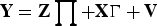
Let us consider a linear IV model with N endogenous regressors, K ≥ N excluded instruments, L included instruments, and T observations as follows:

y = Y β + X k + u (1)

(1)

Y = Z \prod + X Γ + V (2)

(2)

Equation (1) denotes the structural-form relationship between the dependent variable and endogenous regressors, and (2) denotes the first-stage relationship between the endogenous regressors and the instruments. $y \in R^{T \times 1}$ , $Y \in R^{T \times N}$ , $Z \in R^{T \times K}$ , and $X \in R^{T \times L}$ denote, respectively, the matrix of dependent variables, endogenous regressors, excluded instruments, and included instruments. The parameter of interest is $β \in R^{N}$ . $\prod \in R^{K \times N}$ contains the first-stage parameters; $k \in R^{L}$ and $Γ \in R^{L \times N}$ contain coefficients of the included instruments. The intercept term and fixed effects are included in X for notational simplicity.

Substituting Y into the structural form, we have the reduced-form relationship $y = Z \prod β + x α + w$ , where $α = Γ β + k$ and $w = V β + u$ .

Without loss of generality, let us project out the included instruments X. For simplicity, we still use y, Y, Z, u, and V to denote their projection errors onto X. For instance, we replace the endogenous regressors Y by M_XY. We further normalize the instruments such that Z′Z/ T = I _K . The above normalization leaves the 2SLS estimator unchanged. The 2SLS estimator of β is ${\hat{β}}_{2 SLS} = (Y^{'} P_{Z} Y)^{- 1} Y^{'} P_{Z} y$ .

2.1.2 Model assumptions

LM makes the following two assumptions to derive the robust weak-instrument test. First, LM models the weak instruments by assuming that the first-stage relationship is local-to-zero. Second, LM characterizes the asymptotic distributions of reduced-form and first-stage residuals interacted with excluded instruments. The asymptotic covariance W can be any positive definite matrix. Thus, this model allows for arbitrary distributional assumptions on the model errors.

Assumption 1. $\prod = C / \sqrt{T}$ , where $C \in R^{K \times N}$ is a fixed full-rank matrix.

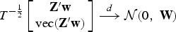
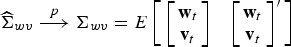
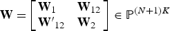
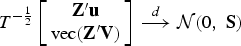
Assumption 2. The following limits hold as T → ∞:

T^{- \frac{1}{2}} [\begin{matrix} Z^{'} w \\ vec (Z^{'} w) \end{matrix}] \overset{d}{⟶} N (0, W)

\hat{W} \overset{p}{⟶} W

{\hat{Σ}}_{w v} \overset{p}{⟶} Σ_{w v} = E [\begin{matrix} [\begin{matrix} w_{t} \\ v_{t} \end{matrix}] & {[\begin{matrix} w_{t} \\ v_{t} \end{matrix}]}^{'} \end{matrix}]

where

W = [\begin{matrix} W_{1} & W_{12} \\ {W^{'}}_{12} & W_{2} \end{matrix}] \in P^{(N + 1) K}

Σ_{w v} = [\begin{matrix} σ_{w}^{2} & σ_{w v} \\ {σ^{'}}_{w v} & Σ_{v} \end{matrix}] \in P^{N + 1}

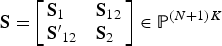
Recalling that w = Vβ+u, let us further define the asymptotic variance of structural-form and first-stage residuals interacted with excluded instruments as S:

T^{- \frac{1}{2}} [\begin{matrix} Z^{'} u \\ vec (Z^{'} V) \end{matrix}] \overset{d}{⟶} N (0, S)

where

S = [\begin{matrix} S_{1} & S_{12} \\ {S^{'}}_{12} & S_{2} \end{matrix}] \in P^{(N + 1) K}

S_{1} = W_{1} + (β^{'} \otimes I_{K}) W_{2} + (β \otimes I_{K}) - (β^{'} \otimes I_{K}) {W^{'}}_{12} + W_{12} (β \otimes I_{K})

S_{12} = W_{12} - (β^{'} \otimes I_{K}) W_{2}

S_{2} = W_{2}

Under assumptions 1 and 2, LM shows that the bias of the 2SLS estimator, ${\hat{β}}_{2 SLS} - β$ , converges in distribution to a limit, denoted by $β_{2 SLS} *$ . Intuitively, the goal of the weak-instrument test is to test whether $E (β_{2 SLS} *)$ is significantly different from zero.

2.1.3 Definition of the weak-instrument set

The following definitions formally introduce the weak-instrument set.Definition 1. The concentration matrix is $Λ = Φ^{- \frac{1}{2}} C^{'} C Φ^{- \frac{1}{2}}$ , where $Φ = {R^{'}}_{N, K} (S_{2} \otimes I_{K}) R_{N, K}$ . Let λ_min = mineval(Λ) be the minimum eigenvalue of Λ.

Definition 1 gives the concentration matrix for a general asymptotic variance matrix W and N ≥ 1. The minimum eigenvalue of this matrix will be used to derive a tractable boundary of the weak-instrument set.

Definition 2. The bias criterion for i ∈ {abs, rel} is $B_{i} = {‖ E (β_{2 SLS} *)^{'} Ξ_{i}^{\frac{1}{2}} ‖}_{2} / \sqrt{b_{i}}$ , where $b_{abs} = σ_{u}^{2}$ , $Ξ_{abs} = Σ_{v}$ ; $b_{rel} = tr (S_{1})$ , $Ξ_{rel} = Φ$ .

LM considers instruments weak when a weighted quadratic loss function of the asymptotic bias $E (β_{2 SLS} *)$ is large in either an absolute or a relative sense. Definition 2 gives the absolute and the relative bias criteria. The choice of weighting matrix $Ξ_{i}$ and scaling factor bi determines whether the bias criterion is expressed in absolute or relative terms. In particular, the absolute bias criterion, B_abs, uses the same weighting and scaling as Stock and Yogo (2005)’s absolute bias criterion. The relative bias criterion, B_rel, is extended from Montiel Olea and Pflueger (2013) and can be interpreted as the asymptotic bias relative to a worst-case benchmark.

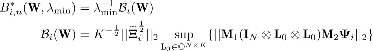
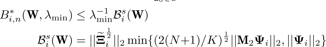
LM applies the standard Nagar (1959) methodology to obtain a tractable proxy for the bias criterion B_i for i ∈ {abs, rel}. They define the Nagar bias as B_i,n and derive the upper bounds on B_i,n for a given λ_min, showing that $B_{i, n} \leq B_{i, n} * (W, λ_{min})$ , where

\begin{aligned} B_{i, n} * (W, λ_{min}) = λ_{min}^{- 1} B_{i} (W) \\ B_{i} (W) = K^{- \frac{1}{2}} {‖ {\tilde{Ξ}}_{i}^{\frac{1}{2}} ‖}_{2} sup_{L_{0} \in O^{N \times K}} {‖ M_{1} (I_{N} \otimes L_{0} \otimes L_{0}) M_{2} ψ_{i} ‖_{2}} \end{aligned}

\begin{aligned} B_{i, n} * (W, λ_{min}) \leq λ_{min}^{- 1} B_{i}^{s} (W) \\ B_{i}^{s} (W) = {‖ {\tilde{Ξ}}_{i}^{\frac{1}{2}} ‖}_{2} min {(2 (N + 1) / K)^{\frac{1}{2}} ‖ M_{2} ψ_{i} ‖_{2}, ‖ ψ_{i} ‖_{2}} \end{aligned}

where

{\tilde{Ξ}}_{i} = Φ^{- \frac{1}{2}} Ξ_{i} Φ^{- \frac{1}{2}}

M_{1} = {R^{'}}_{N, N} {I_{N^{3}} + (K_{N, N} \otimes I_{N})}

M_{2} = R_{N, K} {R^{'}}_{N, K} / (N + 1) - I_{N K^{2}}

ψ_{abs} = (S W_{2}^{- \frac{1}{2}} [{W^{'}}_{12}, {W^{'}}_{2}] \otimes I_{K}) R_{N + 1, K} Σ_{w v}^{- \frac{1}{2}}

ψ_{rel} = (S W_{2}^{- \frac{1}{2}} [{W^{'}}_{12}, {W^{'}}_{2}] \otimes I_{K}) R_{N + 1, K} {{R^{'}}_{N + 1, K} (W \otimes I_{K}) R_{N + 1, K}}^{- \frac{1}{2}}

and

S = {(Φ / K)^{- \frac{1}{2}} \otimes I_{K}} S_{2}^{\frac{1}{2}}

$B_{i} (W)$ forms a sharp upper bound for the Nagar bias B_i,n, which can be obtained through a numerical optimization algorithm by Wen and Yin (2013). $B_{i}^{s} (W)$ forms another nonsharp upper bound that requires no numerical optimization. Section 4.3 discusses the computational burden.

Definition 3. The weak-instrument set for i ∈ {abs, rel} is $B_{i, τ} (W) = {C \in R^{K, N}, β \in R^{N} : B_{i, n} > τ}$ .

Definition 3 describes the weak-instrument set. It depends on the asymptotic variance W, which can be consistently estimated. Because C and β cannot be estimated consistently, the null hypothesis will be tested based on the upper bound of B_i,n.

2.2 Robust weak-instrument test

2.2.1 Null and alternative hypotheses

Given a bias tolerance level τ, LM’s weak-instrument test evaluates whether the minimum eigenvalue of Λ is less than or equal to a threshold value $λ_{min, i} * (τ)$ . Formally, the null and alternative hypotheses are

H_{0} : λ_{min} \leq λ_{min, i} * (τ) versus H_{1} : λ_{min} > λ_{min, i} * (τ)

Where

λ_{min, i} * (τ)

can take the form of either

B_{i} (W) / τ or B_{i}^{s} (W) / τ

. The null hypothesis implies that the Nagar bias is less than or equal to the bias tolerance level τ, that is,

B_{i, n} \leq τ

2.2.2 Test statistic

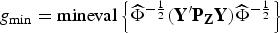
The test statistic is the sample realization of λmin, denoted by gmin.

g_{min} = mineval {{\hat{Φ}}^{- \frac{1}{2}} (Y^{'} P_{Z} Y) {\hat{Φ}}^{- \frac{1}{2}}}

where

\hat{Φ} = {R^{'}}_{N, K} (\hat{W_{2}} \otimes I_{K}) R_{N, K}

LM shows that under assumptions 1 and 2, the test statistic gmin converges in distribution to mineval ${{R^{'}}_{N, K} (ζ \otimes I_{K}) R_{N, K} / K}$ . The random matrix ζ follows a noncentral Wishart distribution $W (d, Σ, Ω)$ with degrees of freedom d = 1, scale matrix $Σ = S S^{'}$ , and noncentrality matrix $Ω = Σ^{- 1} S l l^{'} S^{'} -$ , where $l = S_{2}^{- \frac{1}{2}} vec (C^{'})$ .

2.2.3 Critical value

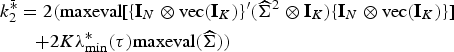
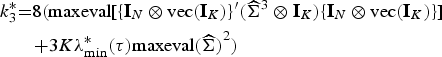
Because of the complexity of the limiting distribution of gmin, it is difficult to derive analytical critical values for the test. LM considers a class of approximating distributions, proposed by Imhof (1961), that match the first three cumulants of the target distribution of gmin. LM shows that the first cumulant of g_min is $k_{1} = K {1 + λ_{min} * (τ)}$ and the upper bounds of the second and third cumulants are

\begin{aligned} k_{2}^{\bar{*}} = 2 (maxeval [{I_{N} \otimes vec (I_{K})}^{'} ({\hat{Σ}}^{2} \otimes I_{K}) {I_{N} \otimes vec (I_{K})}] \\ + 2 K λ_{min} * (τ) maxeval (\hat{Σ})) \end{aligned}

\begin{aligned} k_{3} * = 8 (maxeval [{I_{N} \otimes vec (I_{K})}^{'} ({\hat{Σ}}^{3} \otimes I_{K}) {I_{N} \otimes vec (I_{K})}] \\ + 3 K λ_{min} * (τ) maxeval {(\hat{Σ})}^{2}) \end{aligned}

where $\hat{Σ}$ denotes the matrix obtained by replacing W with $\hat{W}$ in $Σ$ . Moreover, the Imhof (1961) distribution is defined as

F_{I} (x; k_{1}, k_{2}, k_{3}) = F_{χ_{v}^{2}} {(x - k_{1}) 4 ω + v}, v = 8 k_{2} ω^{2}, ω = k_{2} / k_{3}

where

F_{χ_{v}^{2}} (\cdot)

is the cumulative distribution function of a central

χ^{2}

distribution with ν degrees of freedom. The critical value for the robust weak-instrument test at significance level α is the (1 − α) × 100% percentile of the Imhof (1961) distribution with the upper bounds of the cumulants

(k_{2} = k_{2} * and k_{3} = k_{3} *)

. LM proves that these critical values are conservative relative to the unknown critical values from the true distribution of g_min.

Following LM, the weakivtest2 command always verifies that the Kuhn–Tucker conditions of the associated maximization problem are satisfied at the upper bound. If this is not the case, the code numerically solves for the most conservative critical value respecting the bounds. This involves an optimization problem with a nonlinear objective function and linear inequality constraints, which cannot be solved by the built-in Stata optimizer. Therefore, we transform the constrained optimization problem into an unconstrained one using a penalty method (Nocedal and Wright 2006). Section 4.1 shows that the transformation will not alter the optimization result compared with an existing MATLAB package.

2.2.4 Modifications for models with K ≤ N + 1

Because plausible instruments are often scarce, models with only N or N + 1 instruments are of particular practical relevance. However, the bias criterion, B_i, does not exist when K = N. Depending on the assumptions, the bias may not exist when K = N + 1, or it may be difficult to approximate accurately using the Nagar bias, B_i,n. LM provides the following solutions.

For models with K = N + 1, LM recommends using the more conservative bound $λ_{min, i} * (τ) = B_{i}^{s} (W) / τ$ .

For models with K = N, LM recommends testing for the median bias rather than the mean bias. When K = N = 1, LM formally shows that a test based on the median bias of 2SLS can be implemented with the same testing procedure simply by rescaling the tolerance, τ_med = τ /0.455. However, when K = N > 1, a tractable Nagar approximation of median bias cannot be obtained. In this case, LM turns to the more conservative bound.

2.3 Extension to other hypothesis tests

2.3.1 Test for individual elements of ${\hat{β}}_{2 SLS}$

The test using the bias criterion for the full vector ${\hat{β}}_{2 SLS}$ can be modified to test the bias of a single element of ${\hat{β}}_{2 SLS}$ . Denote $e_{j}^{N}$ as the N × 1 vector with the jth element equal to 1 and 0s otherwise. LM defines the bias criterion and weak-instrument set for the jth element in ${\hat{β}}_{2 SLS}$ .

Definition 2-j. The bias criterion for i ∈ {abs, rel} and the jth element in ${\hat{β}}_{2 SLS}$ is $B_{i}^{j} = {‖ {E (β_{2 SLS} *)^{'} e_{j}^{N}} {(e_{j}^{N^{'}} Ξ_{i} e_{j}^{N})}^{\frac{1}{2}} ‖}_{2} / \sqrt{b_{i}}$ .

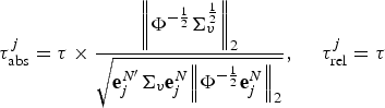
Definition 3-j. The weak-instrument set for i ∈ {abs, rel} and the jth element in ${\hat{β}}_{2 SLS}$ is $B_{i, τ}^{j} (W) = {C \in R^{K \times N}, β \in R^{N} : B_{i, τ}^{j} > τ}$ .

LM shows that under assumptions 1 and 2, the weak instruments test for an individual coefficient can be conducted exactly as the testing procedure in section 2.2, with a simple adjustment to τ,

τ_{abs}^{j} = τ \times \frac{{‖ Φ^{- \frac{1}{2}} Σ_{v}^{\frac{1}{2}} ‖}_{2}}{\sqrt{e_{j}^{N^{'}} Σ_{v} e_{j}^{N} {‖ Φ^{- \frac{1}{2}} e_{j}^{N} ‖}_{2}}}, τ_{rel}^{j} = τ

2.3.2 Tests under local to rank reduction of one

In addition to testing the weak instruments under the local-to-zero assumption, where all instruments are uniformly weak, Sanderson and Windmeijer (2016) consider a local-to-rank-reduction-of-one (LRR1) asymptotic embedding and show that an F statistic proposed by Stock and Yogo (2005) can be used to conduct a bias-based test for models with homoskedastic and serial uncorrelated errors. LM extends the test to allow for heteroskedasticity and autocorrelation. In particular, the LRR1 embedding is formulated as follows.

Assumption 3. The jth column of Π is $\prod_{j} = \prod_{- j} δ + c / \sqrt{T}$ , where $c \in R^{K}$ , $δ \in R^{N - 1}$ , and the matrix $\prod_{- j} \in R^{K \times (N - 1)}$ containing the remaining N − 1 columns of Π is of full column rank.

Assumption 3 indicates that Πj is asymptotically collinear with the remaining columns $\prod_{- j}$ . We emphasize that the results introduced below are valid only under the specific assumed asymptotic embedding given the choice of Πj instead of being uniformly valid under arbitrary rank reductions.

LMs show that under assumptions 2 and 3, the test statistic and critical values for absolute bias of the 2SLS estimator can be constructed using the testing procedure in section 2.2, with the transformed outcome variable $y^{⊥} = M_{{\hat{Y}}_{- j}} y$ , endogenous regressor $y_{j}^{^{⊥}} = M_{{\hat{Y}}_{- j}} y_{j}$ and instruments $Z^{⊥} = M_{{\hat{Y}}_{- j}} \tilde{Z} ({\tilde{Z}}^{'} M_{{\hat{Y}}_{- j}} \tilde{Z} / T)^{- \frac{1}{2}}$ where Yj denotes the jth regressor and Y−j the remaining regressors in Y, ${\hat{Y}}_{- j} = P_{Z} Y_{- j}$ , and $\tilde{Z}$ contains any K − N + 1 columns of Z. Note that the test based on the relative bias criterion under LRR1 asymptotics is not provided.

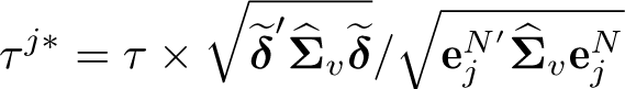
Given the choice of Πj, the test can be further extended to evaluate the absolute bias of the jth element of the 2SLS estimator by adjusting the tolerance level

τ^{j *} = τ \times \sqrt{{\tilde{δ}}^{'} {\hat{Σ}}_{v} \tilde{δ}} / \sqrt{e_{j}^{N^{'}} {\hat{Σ}}_{v} e_{j}^{N}}

where

\tilde{δ}

is such that

{\tilde{δ}}_{j} = 1

and

{\tilde{δ}}_{- j} = ({Y^{'}}_{- j} P_{Z} Y_{- j})^{- 1} {Y^{'}}_{- j} P_{Z} Y_{j}

3 The weakivtest2 command

The command weakivtest2 implements the robust weak-instrument test with multiple endogenous regressors for 2SLS, as developed by LM. It serves as a postestimation command for ivreg2, xtivreg2 (fixed effects only), and ivreghdfe.

weakivtest2 estimates the variance–covariance matrix of errors as specified in the preceding ivreg2, xtivreg2, or ivreghdfe estimation. The following options are supported: 1) robust, which estimates an Eicker–Huber–White heteroskedasticity-robust variance–covariance matrix; 2) robust bw(#), which estimates a heteroskedasticity and autocorrelation consistent (HAC) variance–covariance matrix computed with a Bartlett (Newey–West) kernel; and 3) cluster(varlist), which estimates a variance–covariance matrix clustered on the specified variable.

The weakivtest2 command stores and displays LM’s test statistic and critical values in the Stata Results window. For reference, weakivtest2 stores the test statistic of either Stock and Yogo (2005) or Sanderson and Windmeijer (2016), depending on whether local-to-zero or LRR1 asymptotics are assumed, as well as the critical values based on Nagar approximations when K > N + 1.

3.1 Syntax

The syntax of the weakivtest2 command is as follows:

weakivtest2 I, level(numlist) tau(numlist) asymp totics(string)

crit erion(string) ind ex(#) tar get(#) points(#) fast record ]

3.2 Options

level(numlist) specifies one or more confidence levels 100(1 − α) for the critical values. The default is level(95 90).

tau(numlist) specifies one or more bias tolerance levels τ for the critical values. The default is tau(0.05 0.1 0.2 0.3).

asymptotics(string) chooses the asymptotic embedding used in the test. The option asymptotics(“l0”) corresponds to the L0 embedding, in which all first-stage coefficients are local to zero. The option asymptotics(”lrr1”) corresponds to the LRR1 embedding, in which the first-stage coefficient matrix is local to rank deficiency. The default is asymptotics(“l0”).

criterion(string) selects the bias criterion used to evaluate the Nagar bias. The option criterion(”absolute”) evaluates the bias relative to the maximum ordinary least-squares bias. The option criterion(”relative”) evaluates the bias relative to its worst-case benchmark. The default is criterion(”absolute”). When asymptotics(“lrr1”) is specified, criterion(“absolute”) must be used.

index(#) specifies an integer j (1 ≤ j ≤ N) corresponding to the location of the retained regressor in the vector of endogenous regressors (or Πj in assumption 3), where N is the number of endogenous regressors. This option is required only when asymptotics(“lrr1”) is specified.

target(#) specifies the target of 2SLS coefficients: either 0 for the entire vector ${\hat{β}}_{2 SLS}$ or an integer j (1 ≤ j ≤ N) corresponding to the location of the individual coefficient in ${\hat{β}}_{2 SLS}$ , where N is the number of endogenous regressors. This option must be 0 or the number specified in index() when asymptotics(“lrr1”) is specified. The default is target(0).

points(#) sets the number of random starting points used in the optimization routine to obtain $B_{i} (W)$ . The default is points(1000).

fast requests that only simplified conservative critical values are computed. This option is useful when you want a quick diagnostic; the resulting critical values are guaranteed to be conservative but may be less sharp than the full set of critical values.

record reports the progress of the numerical optimization used to compute the critical values. This option is intended mainly for diagnostic or debugging purposes.

3.3 Stored results

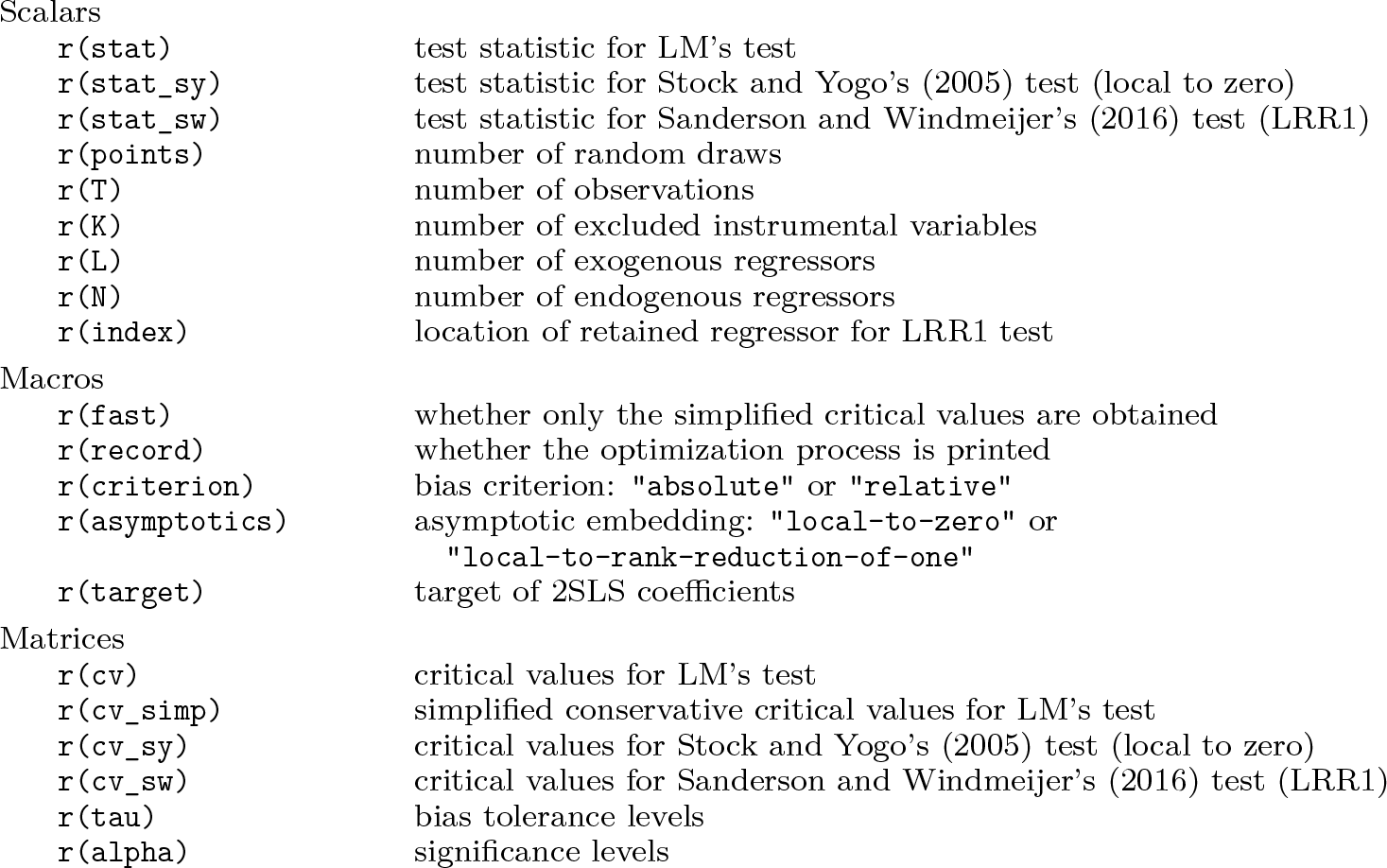
The weakivtest2 command stores the following results in r():

3.4 Relationship with existing commands

The weakivtest2 command is closely related to existing weak-instrument tests for 2SLS in Stata. Section 4.2 investigates the relationship numerically.

Commands ivreg2 (Baum, Schaffer, and Stillman 2007, 2002), xtivreg2 (Schaffer 2005), and ivreghdfe (Correia 2018) report Cragg and Donald’s (1993) Wald F statistic and critical values in Stock and Yogo’s (2005) tables for both bias-and size-based tests, where the critical value for the bias-based test is available only when K > N + 1. weakivtest2 provides the same bias-based test statistic under both relative and absolute bias criteria for models with conditionally homoskedastic and serially uncorrelated errors when K > N + 1. The critical value exhibits some numerical differences because weakivtest2 uses Nagar approximation instead of Monte Carlo integration to evaluate the bias. In addition, weakivtest2 covers models with K ≤ N + 1 by considering median bias for K = N and adopting a conservative bound for K = N + 1. weakivtest2 also reports robust test statistic and critical values for models with general dependence structures in error terms, while those reported by ivreg2, xtivreg2, or ivreghdfe are invalid for these models. Nevertheless, weakivtest2 does not report critical values for the size-based test.

The community-contributed command weakivtest (Pflueger and Wang 2015) reports Montiel Olea and Pflueger’s (2013) effective F statistic and critical values for both 2SLS and limited-information maximum-likelihood estimators when there is a single endogenous regressor. weakivtest2 provides the same test statistic as weakivtest for the 2SLS estimator when N = 1. For models with K > 2 and N = 1, weakivtest2 provides the analytically identical critical value as weakivtest under the relative bias criterion. For models with K = 2 and N = 1, LM recommends using a more conservative bound $B_{rel}^{s} (W)$ , while Montiel Olea and Pflueger (2013) stick with the sharp upper bound $B_{rel} (W)$ . Therefore, weakivtest2 generally provides larger critical values than weakivtest. For models with K = N = 1, the mean bias of 2SLS does not exist. LM considers median bias of the 2SLS estimator, while weakivtest does not make the modification. Therefore, weakivtest2 provides smaller critical values than weakivtest. In addition, weakivtest2 covers models with multiple endogenous regressors N > 1, in which case weakivtest returns an error message. weakivtest2 also allows for the absolute bias criterion instead of the relative bias criterion. Nevertheless, weakivtest2 does not report test results for limited-information maximum-likelihood estimators.

4 Monte Carlo simulations

In this section, we conduct Monte Carlo simulations to investigate the numerical properties of weakivtest2, including its numerical consistency with the MATLAB package, its relationship with other tests in Stata, and its computational burden. We note that the purpose here is not to validate LM’s test. For a comprehensive examination of the size and power of the test, as well as performance comparisons with other tests such as Stock and Yogo (2005) and Montiel Olea and Pflueger (2013), we refer the reader to LM. All simulation results are based on L = 100 replications.

4.1 Consistency with the MATLAB package

In this subsection, we assess the numerical consistency between weakivtest2 and LM’s accompanying MATLAB package, available at gweakivtest.zip (version dated 2025-07-02).

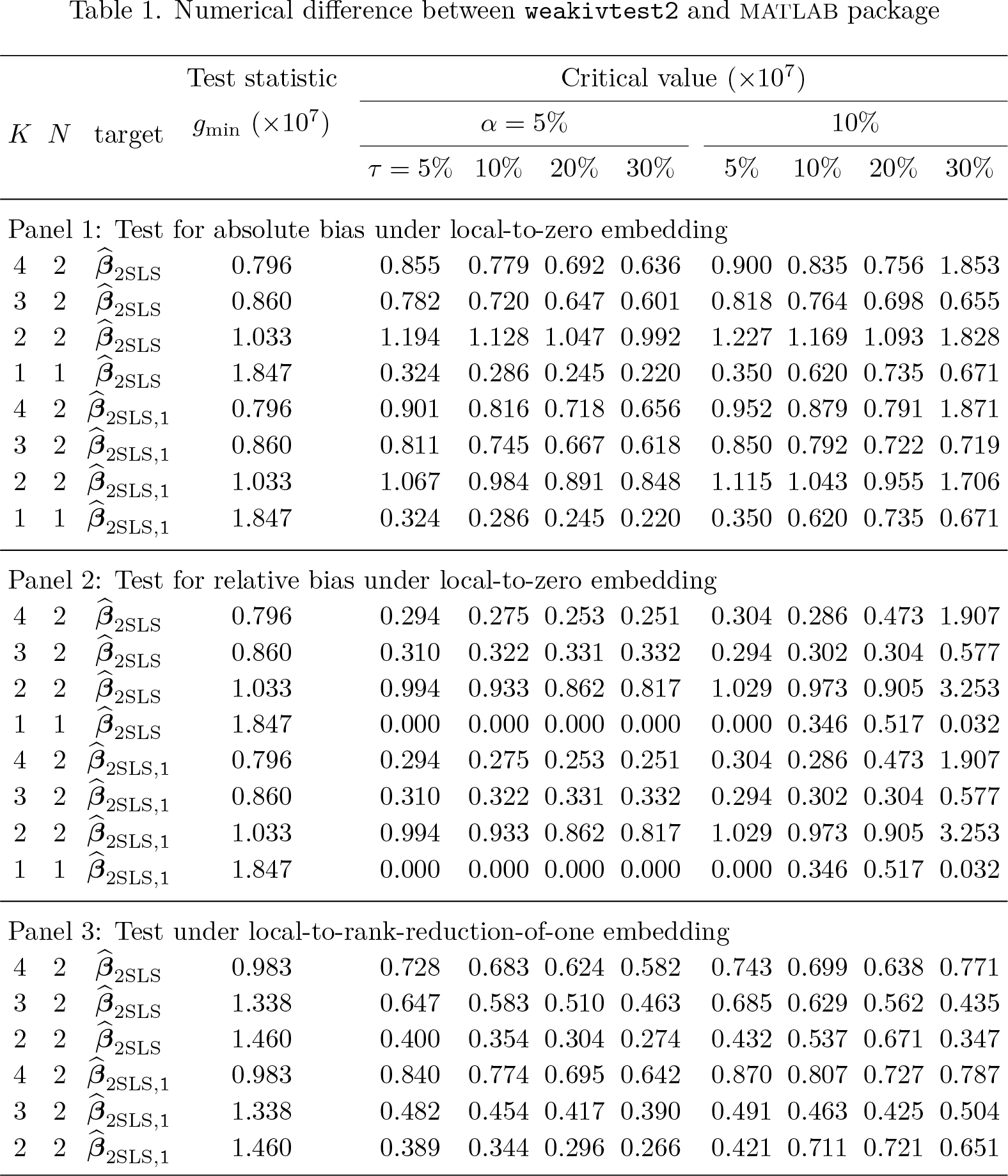
This comparative study considers scenarios that reflect all algorithmic components implemented in weakivtest2. We consider all three types of hypothesis tests: 1) the test for absolute bias under local-to-zero embedding; 2) the test for relative bias under local-to-zero embedding; and 3) the test under LRR1 embedding, retaining the first endogenous regressor. We consider tests for both the full estimator ${\hat{β}}_{2 SLS}$ and the first component of ${\hat{β}}_{2 SLS}$ . We cover four different model sizes: 1) K = 4, N = 2, where the standard algorithm is applied; 2) K = 3, N = 2, where the conservative critical value is calculated; 3) K = N = 2, where the test for median bias is applied with a conservative critical value; and 4) K = N = 1, where the test for median bias is applied with an adjusted tolerance level.

We follow the data generation process (DGP) in gweakivtest_Example.m from the MATLAB package. In particular, we set $β = 1_{N}$ , $k \sim N (0, 1)^{L \times 1}$ , $Γ \sim N (0, 1)^{L \times N}$ , $u \sim N (0, 1)^{T \times 1}$ , $V \sim N (0, 1)^{T \times N}$ , $X \sim [N (0, 1)^{T \times (L - 1)}, 1_{T}]$ , $Z \sim N (0, 1)^{T \times K}$ , and $\prod = \sqrt{0.08 K} \times L_{0}$ , as specified in (1)–(2). We set T = 200 and L = 3 and define $N (0, 1)^{m \times n}$ as an m × n matrix with each element independently drawn from the standard normal distribution. $L_{0} \in R^{N \times K}$ is defined as the first N rows of the K × K orthogonal matrix generated from the QR decomposition of a random matrix $L \sim N (0, 1)^{K \times K}$ .

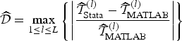
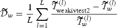
Table 1 reports the scaled numerical difference $\hat{D} \times 10^{7}$ between weakivtest2 and the MATLAB package, using Stata/MP 17 and MATLAB R2023a, respectively. The maximal relative numerical difference $\hat{D}$ is defined as

\hat{D} = max_{1 \leq l \leq L} {| \frac{{\hat{T}}_{Stata}^{(l)} - {\hat{T}}_{MATLAB}^{(l)}}{{\hat{T}}_{MATLAB}^{(l)}} |}

where

{\hat{T}}_{w}^{(l)}

denotes a generic statistic (g_min or critical value) for w ∈ {Stata, MATLAB} in the lth replication. Within each scenario, we report the numerical difference for the test statistic g_min and critical values for α ∈ {0.05, 0.1} and τ ∈ {0.05, 0.1, 0.2, 0.3}. The maximal difference across all scenarios is on the order of 10⁻⁷ or lower, indicating a high degree of numerical equivalence between the Stata and MATLAB implementations.

Table 1.
Numerical difference between weakivtest2 and matlab package

K N target Test statistic $g_{min} (\times 10^{7})$ Critical value (×10⁷)

α = 5% 10%

τ = 5% 10% 20% 30% 5% 10% 20% 30%

Panel 1: Test for absolute bias under local-to-zero embedding

4 2 ${\hat{β}}_{2 SLS}$ 0.796 0.855 0.779 0.692 0.636 0.900 0.835 0.756 1.853

3 2 ${\hat{β}}_{2 SLS}$ 0.860 0.782 0.720 0.647 0.601 0.818 0.764 0.698 0.655

2 2 ${\hat{β}}_{2 SLS}$ 1.033 1.194 1.128 1.047 0.992 1.227 1.169 1.093 1.828

1 1 ${\hat{β}}_{2 SLS}$ 1.847 0.324 0.286 0.245 0.220 0.350 0.620 0.735 0.671

4 2 ${\hat{β}}_{2 SLS, 1}$ 0.796 0.901 0.816 0.718 0.656 0.952 0.879 0.791 1.871

3 2 ${\hat{β}}_{2 SLS, 1}$ 0.860 0.811 0.745 0.667 0.618 0.850 0.792 0.722 0.719

2 2 ${\hat{β}}_{2 SLS, 1}$ 1.033 1.067 0.984 0.891 0.848 1.115 1.043 0.955 1.706

1 1 ${\hat{β}}_{2 SLS, 1}$ 1.847 0.324 0.286 0.245 0.220 0.350 0.620 0.735 0.671

Panel 2: Test for relative bias under local-to-zero embedding

4 2 ${\hat{β}}_{2 SLS}$ 0.796 0.294 0.275 0.253 0.251 0.304 0.286 0.473 1.907

3 2 ${\hat{β}}_{2 SLS}$ 0.860 0.310 0.322 0.331 0.332 0.294 0.302 0.304 0.577

2 2 ${\hat{β}}_{2 SLS}$ 1.033 0.994 0.933 0.862 0.817 1.029 0.973 0.905 3.253

1 1 ${\hat{β}}_{2 SLS}$ 1.847 0.000 0.000 0.000 0.000 0.000 0.346 0.517 0.032

4 2 ${\hat{β}}_{2 SLS, 1}$ 0.796 0.294 0.275 0.253 0.251 0.304 0.286 0.473 1.907

3 2 ${\hat{β}}_{2 SLS, 1}$ 0.860 0.310 0.322 0.331 0.332 0.294 0.302 0.304 0.577

2 2 ${\hat{β}}_{2 SLS, 1}$ 1.033 0.994 0.933 0.862 0.817 1.029 0.973 0.905 3.253

1 1 ${\hat{β}}_{2 SLS, 1}$ 1.847 0.000 0.000 0.000 0.000 0.000 0.346 0.517 0.032

Panel 3: Test under local-to-rank-reduction-of-one embedding

4 2 ${\hat{β}}_{2 SLS}$ 0.983 0.728 0.683 0.624 0.582 0.743 0.699 0.638 0.771

3 2 ${\hat{β}}_{2 SLS}$ 1.338 0.647 0.583 0.510 0.463 0.685 0.629 0.562 0.435

2 2 ${\hat{β}}_{2 SLS}$ 1.460 0.400 0.354 0.304 0.274 0.432 0.537 0.671 0.347

4 2 ${\hat{β}}_{2 SLS, 1}$ 0.983 0.840 0.774 0.695 0.642 0.870 0.807 0.727 0.787

3 2 ${\hat{β}}_{2 SLS, 1}$ 1.338 0.482 0.454 0.417 0.390 0.491 0.463 0.425 0.504

2 2 ${\hat{β}}_{2 SLS, 1}$ 1.460 0.389 0.344 0.296 0.266 0.421 0.711 0.721 0.651

K	N	target	Test statistic $g_{min} (\times 10^{7})$	Critical value (×10⁷)
Panel 1: Test for absolute bias under local-to-zero embedding
4	2	${\hat{β}}_{2 SLS}$	0.796	0.855	0.779	0.692	0.636	0.900	0.835	0.756	1.853
3	2	${\hat{β}}_{2 SLS}$	0.860	0.782	0.720	0.647	0.601	0.818	0.764	0.698	0.655
2	2	${\hat{β}}_{2 SLS}$	1.033	1.194	1.128	1.047	0.992	1.227	1.169	1.093	1.828
1	1	${\hat{β}}_{2 SLS}$	1.847	0.324	0.286	0.245	0.220	0.350	0.620	0.735	0.671
4	2	${\hat{β}}_{2 SLS, 1}$	0.796	0.901	0.816	0.718	0.656	0.952	0.879	0.791	1.871
3	2	${\hat{β}}_{2 SLS, 1}$	0.860	0.811	0.745	0.667	0.618	0.850	0.792	0.722	0.719
2	2	${\hat{β}}_{2 SLS, 1}$	1.033	1.067	0.984	0.891	0.848	1.115	1.043	0.955	1.706
1	1	${\hat{β}}_{2 SLS, 1}$	1.847	0.324	0.286	0.245	0.220	0.350	0.620	0.735	0.671
Panel 2: Test for relative bias under local-to-zero embedding
4	2	${\hat{β}}_{2 SLS}$	0.796	0.294	0.275	0.253	0.251	0.304	0.286	0.473	1.907
3	2	${\hat{β}}_{2 SLS}$	0.860	0.310	0.322	0.331	0.332	0.294	0.302	0.304	0.577
2	2	${\hat{β}}_{2 SLS}$	1.033	0.994	0.933	0.862	0.817	1.029	0.973	0.905	3.253
1	1	${\hat{β}}_{2 SLS}$	1.847	0.000	0.000	0.000	0.000	0.000	0.346	0.517	0.032
4	2	${\hat{β}}_{2 SLS, 1}$	0.796	0.294	0.275	0.253	0.251	0.304	0.286	0.473	1.907
3	2	${\hat{β}}_{2 SLS, 1}$	0.860	0.310	0.322	0.331	0.332	0.294	0.302	0.304	0.577
2	2	${\hat{β}}_{2 SLS, 1}$	1.033	0.994	0.933	0.862	0.817	1.029	0.973	0.905	3.253
1	1	${\hat{β}}_{2 SLS, 1}$	1.847	0.000	0.000	0.000	0.000	0.000	0.346	0.517	0.032
Panel 3: Test under local-to-rank-reduction-of-one embedding
4	2	${\hat{β}}_{2 SLS}$	0.983	0.728	0.683	0.624	0.582	0.743	0.699	0.638	0.771
3	2	${\hat{β}}_{2 SLS}$	1.338	0.647	0.583	0.510	0.463	0.685	0.629	0.562	0.435
2	2	${\hat{β}}_{2 SLS}$	1.460	0.400	0.354	0.304	0.274	0.432	0.537	0.671	0.347
4	2	${\hat{β}}_{2 SLS, 1}$	0.983	0.840	0.774	0.695	0.642	0.870	0.807	0.727	0.787
3	2	${\hat{β}}_{2 SLS, 1}$	1.338	0.482	0.454	0.417	0.390	0.491	0.463	0.425	0.504
2	2	${\hat{β}}_{2 SLS, 1}$	1.460	0.389	0.344	0.296	0.266	0.421	0.711	0.721	0.651

4.2 Comparison with other tests for weak instruments in Stata

In this subsection, we show the relationship between weakivtest2 and other commands designed for testing instrument strength in Stata, following the discussion in section 3.4.

We use the same DGPs as in section 4.1. In addition to the independent and identically distributed (i.i.d.) design, we model serial correlation by drawing u, V, X, and Z from first-order autoregressive processes with mean 0 and variance 1. We fit models with serially correlated errors using the HAC variance–covariance matrix. We consider both absolute and relative bias-based tests, using a significance level of α = 5% and a bias tolerance level of τ = 10%.

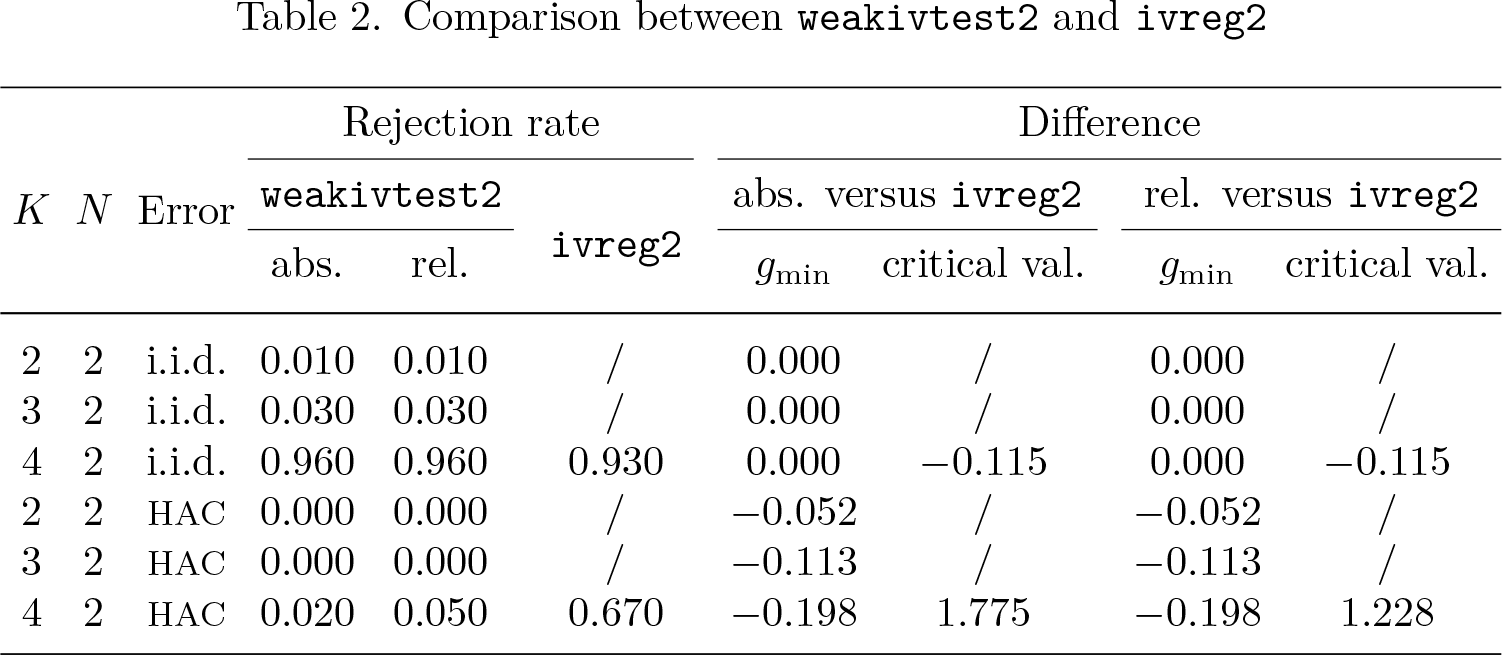
Table 2 compares weakivtest2 with ivreg2, which reports the results of Stock and Yogo’s (2005) test. The first three columns report the average rejection rate, and the remaining four columns report the differences ${\tilde{D}}_{ivreg 2}$ . The numerical difference ${\tilde{D}}_{w}$ is defined as

{\tilde{D}}_{w} = \frac{1}{L} \sum_{l = 1}^{L} \frac{{\tilde{T}}_{weakivtest 2}^{(l)} - {\tilde{T}}_{w}^{(l)}}{{\tilde{T}}_{w}^{(l)}}

where

{\tilde{T}}_{w}^{(l)}

denotes a generic statistic for each w ∈ {ivreg2 , weakivtest , weakivtest2} in the lth replication. The results convey the following. First, for models with K ≤ N + 1, ivreg2 does not provide bias-based critical values, while weakivtest2 fills this gap. Second, for models with K > N + 1 and i.i.d. errors, the two commands generate similar test results with a slight difference, due to different methodologies used to compute the critical values. Finally, for models with K > N + 1 and non-i.i.d. errors, the two commands draw opposite conclusions on the instrument strength. In such a case, we note that LM’s test is theoretically justified, whereas Stock and Yogo’s (2005) test lacks theoretical support.

Table 2.
Comparison between weakivtest2 and ivreg2

K N Error Rejection rate Difference

weakivtest2 ivreg2 abs. versus ivreg2 rel. versus ivreg2

abs. rel. g _min critical val. g _min critical val.

2 2 i.i.d. 0.010 0.010 / 0.000 / 0.000 /

3 2 i.i.d. 0.030 0.030 / 0.000 / 0.000 /

4 2 i.i.d. 0.960 0.960 0.930 0.000 −0.115 0.000 −0.115

2 2 HAC 0.000 0.000 / −0.052 / −0.052 /

3 2 HAC 0.000 0.000 / −0.113 / −0.113 /

4 2 HAC 0.020 0.050 0.670 −0.198 1.775 −0.198 1.228

K	N	Error	Rejection rate	Difference
2	2	i.i.d.	0.010	0.010	/	0.000	/	0.000	/
3	2	i.i.d.	0.030	0.030	/	0.000	/	0.000	/
4	2	i.i.d.	0.960	0.960	0.930	0.000	−0.115	0.000	−0.115
2	2	HAC	0.000	0.000	/	−0.052	/	−0.052	/
3	2	HAC	0.000	0.000	/	−0.113	/	−0.113	/
4	2	HAC	0.020	0.050	0.670	−0.198	1.775	−0.198	1.228

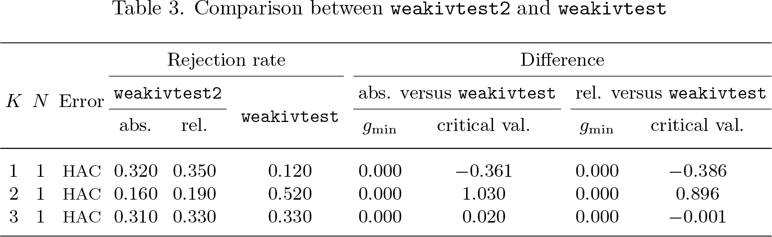
Table 3 compares weakivtest2 with weakivtest, which reports results of Montiel Olea and Pflueger’s (2013) test. The first three columns report the average rejection rate, and the remaining four columns report the differences ${\tilde{D}}_{weakivtest}$ . The results convey the following. First, the test statistics reported by weakivtest2 and weakivtest are identical when N = 1. Second, for models with K = N = 1, weakivtest2 focuses on median bias, resulting in smaller critical values and a higher rejection rate. Third, for models with K = 2 and N = 1, weakivtest2 relies on a more conservative and therefore larger set of critical values, resulting in a lower rejection rate. Fourth, for models with K > N + 1 and N = 1, weakivtest2 generates essentially the same critical value as weakivtest with negligible numerical difference due to different approximation techniques. Montiel Olea and Pflueger (2013) use the Patnaik (1949) approximation to match the first two cumulants. Finally, weakivtest does not provide results when N > 1.

Table 3.

Comparison between weakivtest2 and weakivtest

K	N	Error	Rejection rate			Difference
			weakivtest2		weakivtest	abs.	versus weakivtest	rel.	versus weakivtest
			abs.	rel.	weakivtest	g _min	critical val.	g _min	critical val.
1	1	HAC	0.320	0.350	0.120	0.000	−0.361	0.000	−0.386
2	1	HAC	0.160	0.190	0.520	0.000	1.030	0.000	0.896
3	1	HAC	0.310	0.330	0.330	0.000	0.020	0.000	−0.001

4.3 Computation time

In this subsection, we investigate the computation time of weakivtest2. The main computational burden arises from simulating the sharp upper bound $B_{i} (W)$ via numerical optimization.

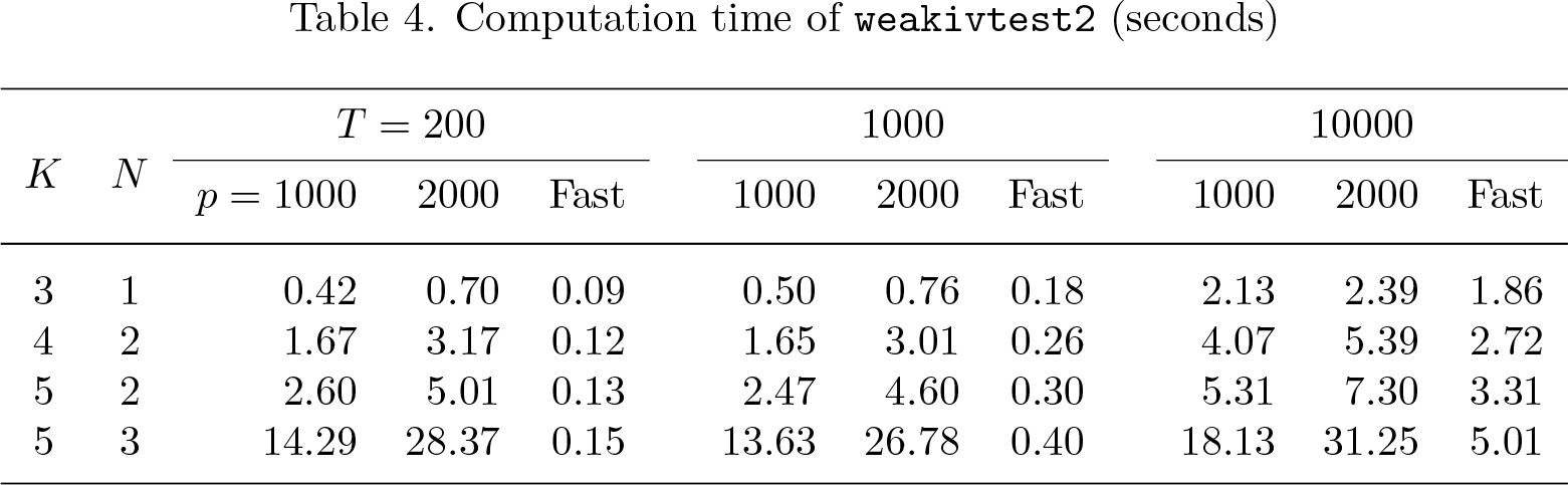
Table 4 reports the computation time of weakivtest2 (without parallel computing) on a MacBook M1 Pro (3.20 GHz and 8-core CPU). The DGPs follow the design described in section 4.1. In general, both the computational power of the machine and the characteristics of the dataset affect the computation time. The number of random draws in obtaining $B_{i} (W)$ (specified by points()), p, linearly increases the computation time, while the sample size T has a smaller effect. In addition, the computation time is negligible when N and K are moderate but increases significantly with model size. If we were to increase the model size—say, to N = 4 and K = 8—the computation time would become prohibitively long. In such cases, the fast option effectively reduces the computation time (at the cost of a more conservative critical value).

Table 4.
Computation time of weakivtest2 (seconds)

K N T = 200 1000 10000s

p = 1000 2000 Fast 1000 2000 Fast 1000 2000 Fast

3 1 0.42 0.70 0.09 0.50 0.76 0.18 2.13 2.39 1.86

4 2 1.67 3.17 0.12 1.65 3.01 0.26 4.07 5.39 2.72

5 2 2.60 5.01 0.13 2.47 4.60 0.30 5.31 7.30 3.31

5 3 14.29 28.37 0.15 13.63 26.78 0.40 18.13 31.25 5.01

K	N	T = 200	1000	10000s
3	1	0.42	0.70	0.09	0.50	0.76	0.18	2.13	2.39	1.86
4	2	1.67	3.17	0.12	1.65	3.01	0.26	4.07	5.39	2.72
5	2	2.60	5.01	0.13	2.47	4.60	0.30	5.31	7.30	3.31
5	3	14.29	28.37	0.15	13.63	26.78	0.40	18.13	31.25	5.01

5 Implementation example

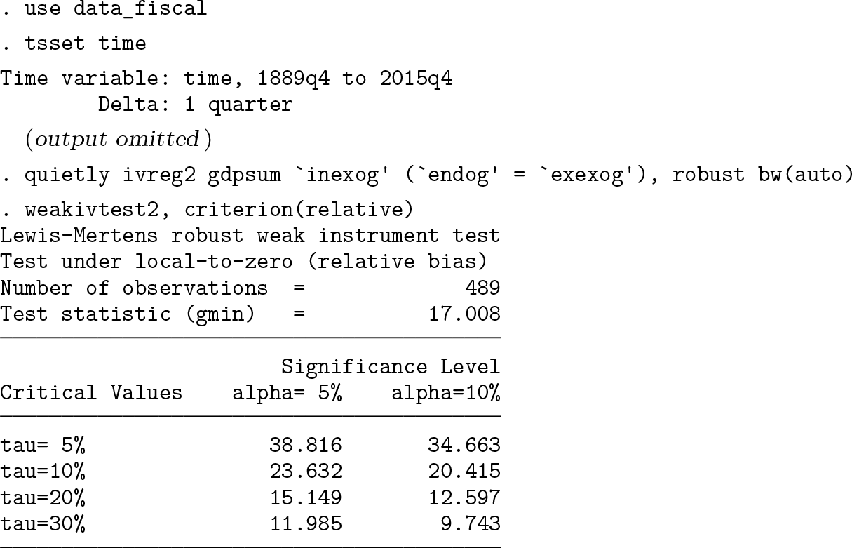
In this section, we follow the empirical application of Ramey and Zubairy (2018) used by LM to illustrate the robust weak-instrument test. Ramey and Zubairy (2018) estimate the state-dependent cumulative government spending multipliers using military news shocks and recursive government spending shocks as instruments. The specification is

\begin{aligned} \sum_{j = 0}^{h} y_{t + j} = I_{t - 1} {γ_{A, h} + ϕ_{A, h} (L) z_{t - 1} + m_{A, h} \sum_{j = 0}^{h} g_{t + j}} \\ + (1 - I_{t - 1}) {γ_{B, h} + ϕ_{B, h} (L) z_{t - 1} + m_{B, h} \sum_{j = 0}^{h} g_{t + j}} + w_{t + h} \end{aligned} (3)

(3)

where h = 0, 1,… is the number of horizons, I is the dummy variable that indicates the state of economy, g is the government spending divided by gross domestic product, y is the detrended gross domestic product, and z is the vector of control variables. The endogenous regressors $I_{t - 1} \times \sum_{j = 0}^{h} g_{t + j}$ and $(1 - I_{t - 1}) \times \sum_{j = 0}^{h} g_{t + j}$ are instrumented by I_t₋₁ × n_t, I_t₋₁ × g_t, (1 − I_t₋₁) × n_t, and (1 − I_t₋₁) × g_t, where n is the military news shock. Therefore, K = 4 and N = 2. Following Ramey and Zubairy (2018), we set h = 12, L = 4, and z_t = (y_t, g_t, n_t). The number of lags in Newey and West’s (1987) HAC model is chosen by Newey and West’s (1994) automatic procedure. We are interested in whether the interest rate is at or near the zero lower bound (ZLB).

The following script implements LM’s weak-instrument test for (3). Because of space limitations, we omit the code used to generate the variables. The local macros endog, inexog, and exexog respectively store the lists of endogenous regressors, included instruments, and excluded instruments.

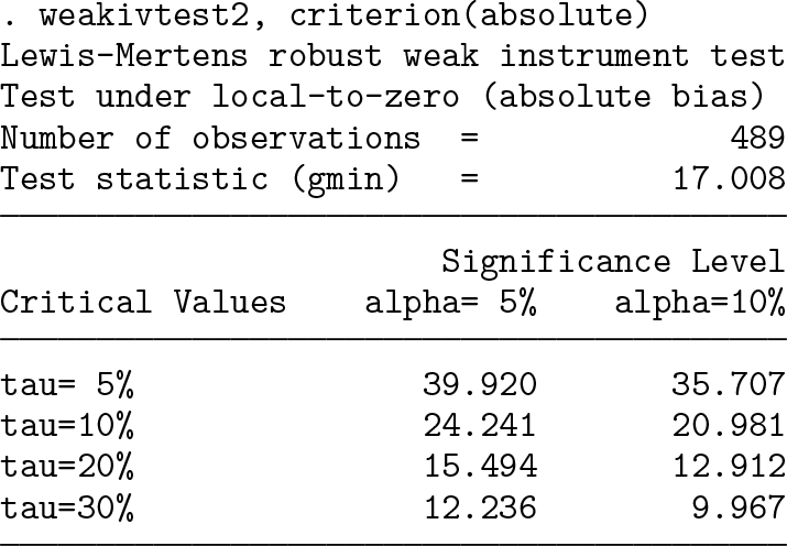
The results indicate that LM’s test statistic is g_min = 17.008, which is smaller than the robust critical value of 23.632 (24.241) under a relative (absolute) bias tolerance level of τ = 10% and a significance level of α = 5%. Therefore, the null hypothesis of weak instruments cannot be rejected.

The result of weakivtest2 can be compared with the results of its related commands, including ivreg2 and weakivtest. On one hand, the ivreg2 command reports a Cragg and Donald’s (1993) Wald F statistic of 28.385, with Stock and Yogo’s (2005) critical values of 7.56 for τ = 10% at a significance level of 5%, indicating that Stock and Yogo’s (2005) test rejects the null hypothesis of weak instruments under an even stricter tolerance level τ . The discrepancy comes from the size distortion of Stock and Yogo’s (2005) test when the model errors are conditionally heteroskedastic and serially correlated, which causes the test to overreject the null hypothesis. The weakivtest2 command gives a more reliable test result when the distributional assumptions on model errors are relaxed.

On the other hand, Pflueger and Wang’s (2015) weakivtest command is inapplicable in this example because of the existence of multiple endogenous regressors. To test instrument strength, Ramey and Zubairy (2018) apply Montiel Olea and Pflueger’s (2013) test to individual subsamples identified by the regime indicators. The regime-specific tests lead to contradictory conclusions. Montiel Olea and Pflueger’s (2013) effective F statistic for the non-ZLB periods is 15.211, with a critical value of 18.311 for τ = 10% at a significance level of 5%, indicating that the instruments are weak. However, the effective F statistic for the ZLB periods is 15.198, with a critical value of 12.698, and thus the null hypothesis of weak instruments is rejected. These conflicting results may cause confusion among practitioners about whether to use weak-instrument robust inference techniques in the subsequent analysis. The weakivtest2 command avoids this dilemma and provides a unified test result on the instrument strength.

6 Conclusions

In this article, I introduced the weakivtest2 command that implements LM’s (Forth-coming) robust test for weak instruments with multiple endogenous regressors in Stata. Given the popularity of IV models, weakivtest2 can be applied to various fields and help the practitioners better evaluate the instrument strength.

The weakivtest2 command is flexible with respect to both the number of endoge-nous regressors and the assumptions on model errors, but it applies only to 2SLS at this stage because of a lack of further theoretical justification. It would be interesting to see the future development of weak-instrument tests for limited-information maximum likelihood and generalized method of moments estimation, along with corresponding statistical software in Stata.

Supplemental Material

sj-txt-2-stj-10.1177_1536867X261425792 - Supplemental material for A robust test for weak instruments with multiple endogenous regressors in Stata

Supplemental material, sj-txt-2-stj-10.1177_1536867X261425792 for A robust test for weak instruments with multiple endogenous regressors in Stata by Lingyun Zhou

Supplemental Material

sj-dta-1-stj-10.1177_1536867X261425792 - Supplemental material for A robust test for weak instruments with multiple endogenous regressors in Stata

Supplemental material, sj-dta-1-stj-10.1177_1536867X261425792 for A robust test for weak instruments with multiple endogenous regressors in Stata by Lingyun Zhou

Footnotes

Acknowledgments

I am grateful to Wenxin Huang and Yiru Wang for their guidance and support. I appreciate the valuable feedback from Daniel Lewis and Luca Sala. I thank the coeditor and the anonymous referee for many constructive comments on the previous version of the article and the command.

7

To install the software files as they existed at the time of publication of this article, type

About the author

Lingyun Zhou is a PhD student in the PBC School of Finance at Tsinghua University.

References

Andrews

Stock

J. H.

Sun

. 2019. Weak instruments in instrumental variables regression: Theory and practice. Annual Review of Economics 11: 727–753. 10.1146/annurev-economics-080218-025643.

Baum

C. F.

Schaffer

M. E.

. 2013. avar: Stata module to perform asymptotic covariance estimation for iid and non-iid data robust to heteroskedasticity, autocorrelation, 1- and 2-way clustering, and common cross-panel autocorrelated disturbances. Statistical Software Components S457689, Department of Economics, Boston College. https://ideas.repec.org/c/boc/bocode/s457689.html .

Baum

C. F.

Schaffer

M. E.

Stillman

. 2002. ivreg2: Stata module for extended instrumental variables/2SLS and GMM estimation. Statistical Software Components S425401, Department of Economics, Boston College. https://ideas.repec.org/c/boc/bocode/s425401.html .

Baum

C. F.

Schaffer

M. E.

Stillman

. 2007. Enhanced routines for instrumental variables/generalized method of moments estimation and testing. Stata Journal 7: 465–506. 10.1177/1536867X0800700402.

Correia

2018. ivreghdfe: Stata module for extended instrumental variable regressions with multiple levels of fixed effects. Statistical Software Components S458530, Department of Economics, Boston College. https://ideas.repec.org/c/boc/bocode/s458530.html .

Cragg

J. G.

Donald

S. G.

. 1993. Testing identifiability and specification in instrumental variables models. Econometric Theory 9: 222–240. 10.1017/S0266466600007519.

Imhof

J. P

. 1961. Computing the distribution of quadratic forms in normal variables. Biometrika 48: 419–426. 10.2307/2332763.

Inoue

Rossi

Wang

. 2024. Has the Phillips curve flattened? CEPR Discussion Paper 18846, Centre for Economic Policy Research. https://cepr.org/publications/dp18846 .

Kleibergen

Paap

. 2006. Generalized reduced rank tests using the singular value decomposition. Journal of Econometrics 133: 97–126. 10.1016/j.jeconom.2005.02.011.

10.

Lewis

D. J.

Mertens

. Forthcoming. A robust test for weak instruments for 2SLS with multiple endogenous regressors. Review of Economic Studies. 10.1093/restud/rdaf103.

11.

Mavroeidis

Plagborg-Møller

Stock

J. H.

. 2014. Empirical evidence on inflation expectations in the New Keynesian Phillips curve. Journal of Economic Literature 52: 124–188. 10.1257/jel.52.1.124.

12.

Montiel Olea

J. L.

Pflueger

C. E.

. 2013. A robust test for weak instruments. Journal of Business and Economic Statistics 31: 358–369. 10.1080/00401706.2013.806694.

13.

Nagar

A. L

. 1959. The bias and moment matrix of the general k-class estimators of the parameters in simultaneous equations. Econometrica 27: 575–595. 10.2307/1909352.

14.

Newey

W. K.

West

K. D.

. 1987. A simple, positive semi-definite, heteroskedasticity and autocorrelation consistent covariance matrix. Econometrica 55: 703–708. 10.2307/1913610.

15.

Newey

W. K.

West

K. D.

. 1994. Automatic lag selection in covariance matrix estimation. Review of Economic Studies 61: 631–653. 10.2307/2297912.

16.

Nocedal

Wright

S. J.

. 2006. Numerical Optimization. 2nd ed. Berlin: Springer. 10.1007/978-0-387-40065-5.

17.

Patnaik

P. B

. 1949. The non-central χ2- and F -distributions and their applications. Biometrika 36: 202–232. 10.1093/biomet/36.1-2.202.

18.

Pflueger

C. E.

Wang

. 2015. A robust test for weak instruments in Stata. Stata Journal 15: 216–225. 10.1177/1536867X1501500113.

19.

Ramey

V. A.

Zubairy

. 2018. Government spending multipliers in good times and in bad: Evidence from US historical data. Journal of Political Economy 126: 850–901. 10.1086/696277.

20.

Sanderson

Windmeijer

. 2016. A weak instrument F -test in linear IV models with multiple endogenous variables. Journal of Econometrics 190: 212–221. 10.1016/j.jeconom.2015.06.004.

21.

Schaffer

M. E.

2005. xtivreg2: Stata module to perform extended IV/2SLS, GMM and AC/HAC, LIML, and k-class regression for panel-data models. Statistical Software Components S456501, Department of Economics, Boston College. https://ideas.repec.org/c/boc/bocode/s456501.html .

22.

Stock

J. H.

Yogo

. 2005. “Testing for weak instruments in linear IV regression”. In Identification and Inference for Econometric Models: Essays in Honor of Thomas Rothenberg, edited by Andrews

D. W. K.

Stock

J. H.

, 80–108. New York: Cambridge University Press. 10.1017/CBO9780511614491.006.

23.

Wen

Yin

. 2013. A feasible method for optimization with orthogonality constraints. Mathematical Programming 142: 397–434. 10.1007/s10107-012-0584-1.

Supplementary Material

Please find the following supplemental material available below.

For Open Access articles published under a Creative Commons License, all supplemental material carries the same license as the article it is associated with.

For non-Open Access articles published, all supplemental material carries a non-exclusive license, and permission requests for re-use of supplemental material or any part of supplemental material shall be sent directly to the copyright owner as specified in the copyright notice associated with the article.

0.00 MB

0.02 MB

K	N	target	Test statistic $g_{min} (\times 10^{7})$	Critical value (×10⁷)
				α = 5%				10%
				τ = 5%	10%	20%	30%	5%	10%	20%	30%
Panel 1: Test for absolute bias under local-to-zero embedding
4	2	${\hat{β}}_{2 SLS}$	0.796	0.855	0.779	0.692	0.636	0.900	0.835	0.756	1.853
3	2	${\hat{β}}_{2 SLS}$	0.860	0.782	0.720	0.647	0.601	0.818	0.764	0.698	0.655
2	2	${\hat{β}}_{2 SLS}$	1.033	1.194	1.128	1.047	0.992	1.227	1.169	1.093	1.828
1	1	${\hat{β}}_{2 SLS}$	1.847	0.324	0.286	0.245	0.220	0.350	0.620	0.735	0.671
4	2	${\hat{β}}_{2 SLS, 1}$	0.796	0.901	0.816	0.718	0.656	0.952	0.879	0.791	1.871
3	2	${\hat{β}}_{2 SLS, 1}$	0.860	0.811	0.745	0.667	0.618	0.850	0.792	0.722	0.719
2	2	${\hat{β}}_{2 SLS, 1}$	1.033	1.067	0.984	0.891	0.848	1.115	1.043	0.955	1.706
1	1	${\hat{β}}_{2 SLS, 1}$	1.847	0.324	0.286	0.245	0.220	0.350	0.620	0.735	0.671
Panel 2: Test for relative bias under local-to-zero embedding
4	2	${\hat{β}}_{2 SLS}$	0.796	0.294	0.275	0.253	0.251	0.304	0.286	0.473	1.907
3	2	${\hat{β}}_{2 SLS}$	0.860	0.310	0.322	0.331	0.332	0.294	0.302	0.304	0.577
2	2	${\hat{β}}_{2 SLS}$	1.033	0.994	0.933	0.862	0.817	1.029	0.973	0.905	3.253
1	1	${\hat{β}}_{2 SLS}$	1.847	0.000	0.000	0.000	0.000	0.000	0.346	0.517	0.032
4	2	${\hat{β}}_{2 SLS, 1}$	0.796	0.294	0.275	0.253	0.251	0.304	0.286	0.473	1.907
3	2	${\hat{β}}_{2 SLS, 1}$	0.860	0.310	0.322	0.331	0.332	0.294	0.302	0.304	0.577
2	2	${\hat{β}}_{2 SLS, 1}$	1.033	0.994	0.933	0.862	0.817	1.029	0.973	0.905	3.253
1	1	${\hat{β}}_{2 SLS, 1}$	1.847	0.000	0.000	0.000	0.000	0.000	0.346	0.517	0.032
Panel 3: Test under local-to-rank-reduction-of-one embedding
4	2	${\hat{β}}_{2 SLS}$	0.983	0.728	0.683	0.624	0.582	0.743	0.699	0.638	0.771
3	2	${\hat{β}}_{2 SLS}$	1.338	0.647	0.583	0.510	0.463	0.685	0.629	0.562	0.435
2	2	${\hat{β}}_{2 SLS}$	1.460	0.400	0.354	0.304	0.274	0.432	0.537	0.671	0.347
4	2	${\hat{β}}_{2 SLS, 1}$	0.983	0.840	0.774	0.695	0.642	0.870	0.807	0.727	0.787
3	2	${\hat{β}}_{2 SLS, 1}$	1.338	0.482	0.454	0.417	0.390	0.491	0.463	0.425	0.504
2	2	${\hat{β}}_{2 SLS, 1}$	1.460	0.389	0.344	0.296	0.266	0.421	0.711	0.721	0.651

K	N	Error	Rejection rate			Difference
			weakivtest2		ivreg2	abs.	versus ivreg2	rel.	versus ivreg2
			abs.	rel.	ivreg2	g _min	critical val.	g _min	critical val.
2	2	i.i.d.	0.010	0.010	/	0.000	/	0.000	/
3	2	i.i.d.	0.030	0.030	/	0.000	/	0.000	/
4	2	i.i.d.	0.960	0.960	0.930	0.000	−0.115	0.000	−0.115
2	2	HAC	0.000	0.000	/	−0.052	/	−0.052	/
3	2	HAC	0.000	0.000	/	−0.113	/	−0.113	/
4	2	HAC	0.020	0.050	0.670	−0.198	1.775	−0.198	1.228

K	N	T = 200			1000			10000s
K	N	p = 1000	2000	Fast	1000	2000	Fast	1000	2000	Fast
3	1	0.42	0.70	0.09	0.50	0.76	0.18	2.13	2.39	1.86
4	2	1.67	3.17	0.12	1.65	3.01	0.26	4.07	5.39	2.72
5	2	2.60	5.01	0.13	2.47	4.60	0.30	5.31	7.30	3.31
5	3	14.29	28.37	0.15	13.63	26.78	0.40	18.13	31.25	5.01

A robust test for weak instruments with multiple endogenous regressors in Stata

Abstract

Keywords

1 Introduction

2 Econometric framework

2.1 Model setup

2.1.1 Linear IV models

2.1.3 Definition of the weak-instrument set

2.2 Robust weak-instrument test

2.2.1 Null and alternative hypotheses

2.2.2 Test statistic

2.2.3 Critical value

2.2.4 Modifications for models with K ≤ N + 1

2.3 Extension to other hypothesis tests

2.3.1 Test for individual elements of β ^ 2 SLS

2.3.2 Tests under local to rank reduction of one

3 The weakivtest2 command

3.1 Syntax

3.2 Options

3.3 Stored results

3.4 Relationship with existing commands

4 Monte Carlo simulations

4.1 Consistency with the MATLAB package

Supplemental Material

sj-txt-2-stj-10.1177_1536867X261425792 - Supplemental material for A robust test for weak instruments with multiple endogenous regressors in Stata

Supplemental Material

sj-dta-1-stj-10.1177_1536867X261425792 - Supplemental material for A robust test for weak instruments with multiple endogenous regressors in Stata

Footnotes

Acknowledgments

7

About the author

References

Supplementary Material

2.3.1 Test for individual elements of ${\hat{β}}_{2 SLS}$