Geometric Total Plaque Area Is an Equally Powerful Phenotype Compared With Carotid Intima-Media Thickness for Stroke Risk Assessment: A Deep Learning Approach

Abstract

Currently, carotid intima-media thickness (cIMT) and geometric total plaque area (gTPA) are computed manually and thus are tedious and prone to interobserver and intraobserver variabilities. This study presents an intelligence-based automated deep learning (DL)–based technique for carotid wall interface detection, cIMT, and lumen diameter (LD) measurements, followed by a 3D cylindrical approach for TPA measurement. The observers were used for manual tracings of which were then used for the design of two DL-based systems. The DL boundaries for inner lumen wall and outer interadventitial borders were used for computing the cIMT and LD. Using cylindrical approach, we computed the gTPA. Furthermore, we compute the 10-year image-based cIMT and gTPA, using the progression rates. A total of 396 B-mode ultrasound right and left common carotid artery images were taken from 203 patients. The mean cIMT and gTPA using DL1 and DL2 is 0.91 mm, 20.52 mm² and 0.88 mm, 19.44 mm², respectively. The coefficient of correlation between gTPA and cIMT using DL1 and DL2 is 0.92 (P < .001) and 0.94 (P < .001), respectively. The area under the curve (AUC) for gTPA showed an improvement over cIMT by 14.36% and 12.57% for DL1 and DL2, respectively. The corresponding 10-year risk improvements were 9.09% and 6.26%. Our statistical significance tests successfully passed t test, Mann-Whitney, Wilcoxon, Kolmogorov-Smirnov, and Friedman. The study shows gTPA as an equally powerful carotid risk biomarker like cIMT. Given the cIMT and LD, cylindrical fitting is a fast method for gTPA measurements.

Keywords

stroke carotid artery plaque risk biomarkers ultrasound common carotid cylinder fitting cIMT gTPA

Introduction

Cardiovascular diseases (CVD) are prevalent in both developing and developed countries. The mortality rate due to CVD is about 5 million each year.¹ In the United States, there is a death due to heart attack or stroke in every 43 seconds and the financial toll is 53.6 billion² US dollars a year, which includes both direct and indirect costs.

The cause of the stroke and myocardial infarction³ is due to the lack of oxygenated blood supply in the brain and heart through the arteries. This is due to the plaque formation in the arterial wall and the disease is called atherosclerosis.⁴ Both external (environmental such as pollution) and internal factors^4,5 (such as lipid formation, genetics, diabetes, hypertension, cholesterol, and rheumatoid arthritis) contribute to this disease formation.^5,6

The stenosis in the arterial walls can be imaged using several imaging modalities such as magnetic resonance imaging (MRI), computed tomography (CT), and ultrasound (US), of which US offers several advantages such as low cost, user friendliness, and diagnosis.^7-9 With advancement in image reconstruction technology such as US beam formation, one can obtain a high resolution US image depicting the arterial lesions. The quantification of these lesions can act as a risk biomarker for carotid artery disease. Thus, one requires an advanced set of tools for the quantification of these carotid artery disease risk biomarkers.

Carotid intima-media thickness (cIMT) is one of the most popular and well established and proven biomarkers that is used for monitoring stroke and cardiovascular risk.^3,10-12 Based on the experience of the authors, most of the clinics or US vascular laboratories around the globe either use manual methods or semi-automated methods for cIMT measurement. These methods require the sonographer (or sonologist or a radiologist) to place the region of interest (ROI) window in the far wall (either distal or mid or proximal) of the carotid artery.

Recently, the second identified biomarker, so-called total plaque area (TPA), has shown to have its link with stroke and cardiovascular risk.^13-16 These studies measure TPA in longitudinal CCA (common carotid artery) US scans using manual methods such as mouse tracings of the media region along with the plaque that is above the baseline. Because the manual cIMT and TPA computations are tedious and prone to interobserver and intraobserver variabilities, there is need of fast, automated, and accurate strategy for both cIMT and TPA measurements. This study is focused on development of such automated cIMT and TPA measurements. Note that TPA can be sometimes be misguided by an index such “total plaque burden,” which is computed in the transverse (or cross-sectional) US scans (perpendicular to blood flow) summed over all the transverse slices. We are computing the far region between lumen-intima (LI) and media-adventitia (MA) in US scans including region above the focal thickening, thereby defining that to be TPA, which is very much along the lines defined by Spence et al,^14,15 Rundek et al,¹⁶ Mathiesen et al,^17-19 and Adams et al.^20-21

Interestingly, the shape of the carotid artery resembles a cylinder, with a fixed thickness. Therefore, one can model the measurement of TPA by fitting a 3D cylinder in the carotid artery with a uniform thickness.¹⁶ As the mid CCA section has a cylindrical geometry, we therefore hypothesize that fast and accurate TPA computations are possible in the mid and proximal regions of the carotid artery. The thickness of the cylinder can be computed by taking the difference between the outer and inner cylinder. In Figure 1, the area of the intima-media complex (IMC) for the far wall is computed by subtracting the inner cylinder from the outer cylinder. This outer cylindrical area along the length of the carotid artery is a function of lumen diameter (LD) and thickness of the cylinder (cIMT). Similarly, the inner cylindrical area will be a function of lumen diameter (D). As a result, all we need both cIMT and LD computations for the TPA measurements.

Figure 1.

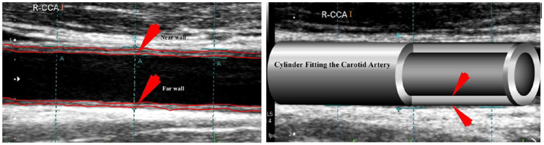
Left: IMT complex for the near and far wall. Right: Computer-assisted CCA.

For cIMT computation, we have used a standard intelligence-based, deep learning (DL)–based technique for automated carotid wall interface detection followed by cIMT and TPA measurements. Since DL paradigms require manual tracings to train the neural network, we have adapted 2 different manual tracers for the DL design. This leads to 2 sets of DL systems. The DL system captures plaque morphology along the carotid walls (typically carotid mid or carotid proximal subsections of the carotid artery) and cIMT is measured using the automated standardized polyline distance method.^22,23 As the wall interfaces for LI and MA are all along the morphology of the plaque, the TPA computations are therefore labeled as morphologic TPA (mTPA) (Appendix B). As explained earlier, mTPA is a function of LD and cIMT. From here, we will call LD as D, representing diameter.²⁴ The advantage of geometric total plaque area (gTPA) is its fast computation due to cylindrical-fitting approach. Note that our study presents a novel and DL-based fast solution using cylinder-based method for an automated cIMT and gTPA computation for CCA only. Such models are truly helpful in subclinical atherosclerosis monitoring, especially, the real world clinics that normally adapt CCA for their subclinical atherosclerosis monitoring. Furthermore, since CCA scans can have positive slope and negative slope in US scans, such models are very helpful since the shape still resembles 3D cylinder. Note that our model is only applicable to CCA, unlike bulb or ICA as defined by Suri et al.^25,26 The second novelty lies in computing the 10-year risk using image-based phenotypes due to its simplicity, unlike considering conventional cardiovascular risk (CCVR) factors. Note that this study is focused only on the 2D longitudinal CCA-based paradigm for gTPA computation, due to its popularity and adaptability in the US industry, unlike 3D-based plaque imaging. The novelty of this article is more on gTPA rather more on an engineering context. The novelty design of DL and benchmark-related validations are published with Elsevier (computers in biology and medicine).²⁷ As it is already published, we did not reproduce the same again.

Our contribution is demonstrated in Figure 2. The pipeline consists of 3 phases: (1) cIMT and LD measurement, (2) gTPA measurement, and (3) risk stratification and assessment.

Figure 2.

Main pipeline, global picture of the system.

Performance Numbers

Our system demonstrates that the coefficient of correlation (CC) between gTPA and cIMT using DL and manual was 0.92 (P < .001) and 0.94 (P < .001), respectively. Using 2 cutoffs leading to low, moderate, and high risk assessment system, the area under the curve (AUC) for cIMT and gTPA was 0.76 (P < .001) and 0.85 (P < .001) using DL1 and 0.76 (P < .001) and 0.86 (P < .001) using DL2, respectively. The gTPA is an equally powerful carotid risk biomarker like cIMT. Given the cIMT and LD, cylindrical fitting is a fast method for gTPA measurements.

The article is organized as follows. “Background Survey on cIMT, LD, and TPA Measurements” section presents background survey related to IMT, LD, and TPA, and “Materials and Methodology” section shows materials and methods used for gTPA computation. “Experimental Protocol, Results, and Its Validation” section presents the results and “Statistical Tests and 10-year Risk Analysis” section demonstrates statistical tests and correlation plots. “Discussion” section explains discussions on result and hypothesis validation. Finally, the “Conclusions” section presents the conclusion and future directions. Note that the symbols used in all mathematical equations are discussed in Appendix E.

Background Survey on cIMT, LD, and TPA Measurements

cIMT Detection and Measurement Methods

Several studies had tried for LI/MA detection of the carotid far wall and corresponding cIMT measurements. Molinari et al²³ proposed automated techniques for cIMT measurement. The Completely Automated Multiresolution Edge Snapper (CAMES) was designed on a multiresolution-based approach and utilized the concept of scale-space. The Completely Automated Layers EXtraction (CALEX) method²⁸ is integrated with feature extraction, line fitting, and classification. The second method was Completely Automated Robust Edge Snapper (CARES) that combines feature extraction and edge detection paradigm.²⁹ Furthermore, the fourth method was a system of Carotid Automated Double-Line Extraction System based on Edge-Flow (CAUDLES-EF).³⁰

Previous methods utilized edge detection technique with US texture and edge energies. In the year 2012, Suri and Saba et al³¹ proposed an automated system AtheroEdge™ for automated cIMT measurement. The study used scale-space strategy for the computation of cIMT. Ikeda et al,³² in 2015, proposed a combination of global and local strategy with texture-based entropy and morphology for cIMT measurement along with classification paradigm. In 2016, Saba et al³³ developed an automated cloud-based solution AtheroCloud^TM for cIMT measurement. Recently in 2017, Ikeda et al²⁵ used the bulb edge point as a reference marker and proposed an automated segmental-cIMT measurement technique. The above-discussed methods depend on features such as grayscale median and calcium area for automated cIMT computation for risk assessment. The external factors make these spatial methods prone to interoperator and intraoperator observer variability and reproducibility study and lack with robust system.

The DL-based system removes some limitations in US imaging technology. The neural networks intelligence power is used to gain shape information from carotid US cohorts. It helps to take advantage of multiresolution approaches for increased processing speed and feature extraction at multiple scales, and thus improves spatial deck of information. Current imaging techniques experience challenges in feature extraction due to the presence of calcium in near wall and due to the shadows in the far wall. This results in the LI, MA border position errors, and cIMT error. Even though previous methods did employ multiresolution-based approaches for increasing the processing speed, the feature extraction at multiple scales was not derived, thus lacking a comprehensive spatial deck of information. Furthermore, carotid US cohorts have shape information which can be learnt via neural networks, intelligence power of which is well established. The current DL-based study removes all the above challenges and thus provides reliability and robustness to the system. This study is motivated by previous works of Suri and his team who had applied machine intelligence in different fields of medicine such as gynecology, urology, dermatology, neurology,^34-37 and recently in endocrinology area.³⁸

LD Detection and Measurement Methods and Our Proposal

Previous literature has also tried several methods for LD measurement. Molinari et al²⁸ used 4 points of the ROI using Hough transform. However, the algorithm performance is limited in the case of less-bright images where the lumen region may not get detected at all. The study used an integrated approach for geometric feature extraction, line fitting, and classification to extract the CCA. However, the final algorithm outcome is affected by noise and presence of similar echo graphic structures (such as jugular vein) and fails in classification of final line pairs, ie, CCA near wall (also known as LI-near) and CCA far (also known as LI-far) wall. Loizou et al³³ introduced snake-based approach for the CCA segmentation but it suffered from initialization and boundary leakage problem.^34,35 Araki et al³⁶ combined the scale-space approach with level set for determining the lumen borders. Kumar et al³⁹ used combination of spatial transformation and scale-space-based approach to estimate the LI-far wall and LI-near wall. The major drawback of the above-discussed methodologies used is lack of intelligence-based approach in their models. Furthermore, they also lack the accumulated information from the population required for intelligent learning by the system. The earlier systems also lacked model-based imaging which is required for full automation. These limitations demand an immediate need for intelligence-based reliable, accurate, and robust method for LD measurement, which can be used as an indicator of atherosclerotic build-up for predicting the risk of stroke. Current study is focused on the results evaluated by an automated LD measurement using DL paradigm, a class of AtheroEdge™ (AtheroPoint™, Roseville, California) system in CCA. We are motivated by training-based learning strategies in the field of classification and segmentation of US images. Extreme learning machine (ELM) and support vector machines (SVM) have been used successful in characterization and stratification of US Fatty Liver Disease (FLD) images.⁴⁰ However, they do not produce accurate results in case of segmentation as they depend on conventional feature extraction techniques. We thus introduce the results of DL-based system⁴¹ for CCA lumen segmentation from US images. The main benefit of using DL is that it is independent from conventional feature generation techniques. This is because DL system generates features internally. In this article, we had applied 3-stage DL-based model for results evaluation.

TPA grows all around the artery tree which causes life-threatening cardiovascular events. We hypothesize that cylindrical-fitting method covers the larger cylinder area for plaque burden calculation in arteries. Intelligence-based cIMT and LD computations using the DL framework can provide better results in comparison with the conventional exiting systems.

Assumptions

Our TPA^8,42-43 by default is only relevant to the longitudinal plane taken from clavicle bone to jaw in the neck region. Even though the carotid artery^28,30 has 3 segments (ICA, Bulb, CCA-distal, CCA-mid, CCA-proximal), our model assumes CCA region for gTPA measurement, along the lines as reported by Spence et al,^14,15 Rundek et al,¹⁶ Mathiesen et al,¹⁷ Herder et al,¹⁸ Kamycheva et al,¹⁹ Romanens et al,²⁰ and Adams et al.²¹ Further due to simplicity of projection rates for cIMT, we only consider image-based projection rates for computing the 10-year risk, unlike adding the CCVR factors.

Materials and Methods

Patient Demographics and Image Acquisition

The study consisted of 204 patients (157M/47F; mean age: 69 ± 11 years) ranging between 29 and 88 years. The database consisted of a total of 396 images out of the supplied 407 left and right carotid images taken from 204 patients. Both left and right CCA retrospectively analyzed by 2 operators (novice and experienced). Table 1 shows the detail of the patient demographics.

Table 1.

Patient Demographics.

Demographic variables	Men (n = 157) mean	Women (n = 47) mean	Combined mean
Age (years)	67.0 ± 11.0	75.3 ± 8.4	68.9 ± 11.0
Rt mean cIMT (mm)	1.0 ± 0.5	1.1 ± 0.4	1.1 ± 0.5
Lt mean cIMT (mm)	1.2 ± 0.5	1.2 ± 0.5	1.2 ± 0.5
Plaque score	8.9 ± 5.5	9.1 ± 4.8	9.0 ± 5.3
LDL cholesterol (mg/dL)	100.0 ± 31.9	105.1 ± 29.9	101.1 ± 31.5
HDL cholesterol (mg/dL)	48.1 ± 13.2	59.0 ± 18.1	50.5 ± 15.0
eGFR (µmol/L)	42.2 ± 18.6	56.0 ± 24.2	45.3 ± 20.8
Calcium (%)	2.8 ± 2.8	3.5 ± 2.7	2.8 ± 2.2
History of CVD (%)	13.2	8.5	21.7
Denovo	1.0 ± 0.0	1.0 ± 0.0	1.0 ± 0.0
HT (mm Hg)	0.7 ± 0.5	0.7 ± 0.4	0.7 ± 0.4
DM	0.3 ± 0.5	0.2 ± 0.4	0.3 ± 0.4
Dyslipidemia	0.6 ± 0.5	0.4 ± 0.5	0.6 ± 0.5
Family History	0.1 ± 0.3	0.1 ± 0.3	0.1 ± 0.3
HD	0.1 ± 0.3	0.1 ± 0.3	0.1 ± 0.3
Smoking	0.5 ± 0.5	0.1 ± 0.4	0.4 ± 0.5
FBS	121.7 ± 34.1	119.2 ± 38.1	121.1 ± 34.9
HbA1c (mg/dL)	6.3 ± 1.2	6.3 ± 0.9	6.3 ± 1.1
Cr	1.7 ± 2.1	1.3 ± 1.9	1.6 ± 2.1

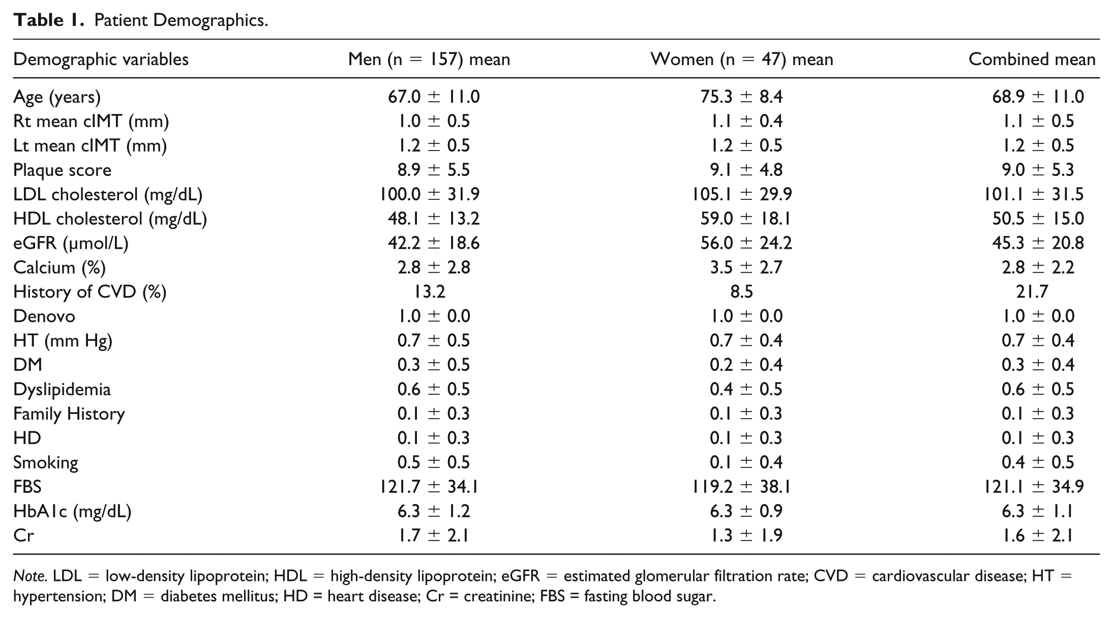
Note. LDL = low-density lipoprotein; HDL = high-density lipoprotein; eGFR = estimated glomerular filtration rate; CVD = cardiovascular disease; HT = hypertension; DM = diabetes mellitus; HD = heart disease; Cr = creatinine; FBS = fasting blood sugar.

The patient’s data and the ethical approval were granted by Toho University Institutional Review Board (IRB), Japan. The data collection and preparation was carried out between July 2009 and December 2010. A total of 11 images were rejected due to lack of tissue information in the grayscale US scans. The cohort consisted of mean HbA1c level of 6.30 ± 1.1% (ranging between 4.8% and 13.0%), total cholesterol of 175.39 ± 38.26 (mg/dL) (ranging between 61 mg/dL and 297 mg/dL), low-density lipoprotein cholesterol (LDL-C) of 101.16 ± 31.79 (mg/dL) (ranging between 24 and 193 mg/dL), and high-density lipoprotein cholesterol (HDL-C) of 50.59 ± 15.13 (mg/dL) (ranging between 18 and 115 mg/dL). From the pool of 203 patients, 92 patients were regular smokers. The hypertensive and high cholesterol patients were on adequate medication: Statin was prescribed for 93 patients to lower the cholesterol levels and 84 of them received renin angiotensin system antagonists. The blood pressure statistics of the patients were not available.

A sonographic scanner (Aplio XV, Aplio XG, Xario; Toshiba, Inc, Tokyo, Japan) equipped with a 7.5-MHz linear array transducer was employed to examine the left and right carotid arteries. All scans were performed under the supervision of an experienced sonographer (with 15 years of experience). High-resolution images were acquired as per the recommendations by the American Society of Echocardiography Carotid Intima Media Thickness Task Force. The mean pixel resolution of the database was 0.05 ± 0.01 mm/pixel. This Japanese diabetic cohort had 148 patients diagnosed with hypertension, 118 patients with dyslipidemia, and 83 were smokers. Out of total patients, 108 patients had proximal lesion location, 29 had at distal, and 67 had at mid lesion location in CCA.

gTPA Modeling Using Cylindrical Fitting

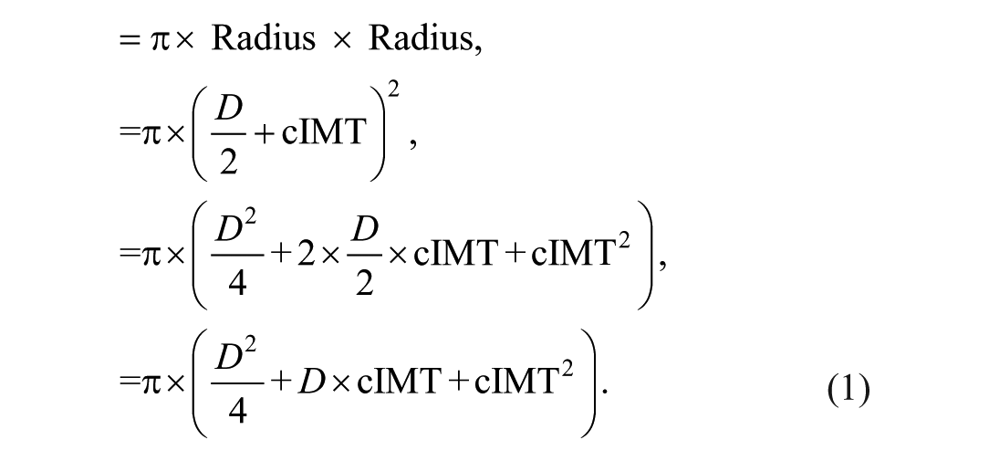
In this section, we analyze the relationship between gTPA, LD, and cIMT. The basic idea is to compute the cylindrical outer and inner area and to subtract them take a difference to compute the mTPA. Outer area of the circular risk can be used for the outer cylinder as represented in equations 1 to 3:

Outer lumen area (LA_outer) of the circle along the LA (longitudinal axis)

\begin{array}{l} = π \times Radius \times Radius, \\ = π \times {(\frac{D}{2} + cIMT)}^{2}, \\ = π \times (\frac{D^{2}}{4} + 2 \times \frac{D}{2} \times cIMT + {cIMT}^{2}), \\ = π \times (\frac{D^{2}}{4} + D \times cIMT + {cIMT}^{2}) . \end{array}

(1)

Inner lumen area (LA_inner) of the circle along the LA (longitudinal axis):

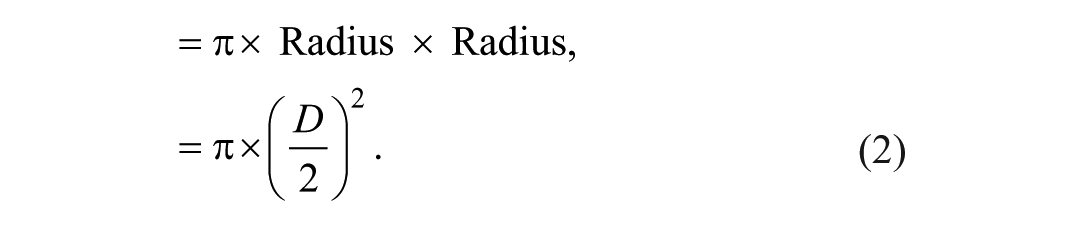
\begin{array}{l} = π \times Radius \times Radius, \\ = π \times {(\frac{D}{2})}^{2} . \end{array}

(2)

Total area of IMT complex:

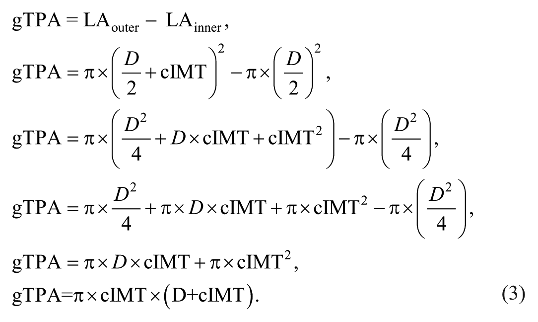
\begin{array}{l} gTPA = {LA}_{outer} - {LA}_{inner}, \\ gTPA = π \times {(\frac{D}{2} + cIMT)}^{2} - π \times {(\frac{D}{2})}^{2}, \\ gTPA = π \times (\frac{D^{2}}{4} + D \times cIMT + {cIMT}^{2}) - π \times (\frac{D^{2}}{4}), \\ gTPA = π \times \frac{D^{2}}{4} + π \times D \times cIMT + π \times {cIMT}^{2} - π \times (\frac{D^{2}}{4}), \\ gTPA = π \times D \times cIMT + π \times {cIMT}^{2}, \\ gTPA= π \times cIMT \times (D+cIMT) . \end{array}

(3)

Thus, gTPA is a function of cIMT and lumen diameter.

Overall Architecture

The expanded version of the overall system (Figure 2) is shown in Figure 3. There are the 3 fundamental stages. Stage 1 consists of cIMT and LD border estimation using DL paradigm, given the gold standard manual tracings of cIMT and LD. A detailed discussion of stage 1 is provided in the next subsection. The main focus of stage 2 is to compute gTPA based on cIMT and LD measurements, which in turn is computed using standardized polyline distance method (Appendix B). The process of gTPA computation in stage 2 is called IMT complex and is performed using the cylindrical-fitting approach. Given the ground truth manual readings for cIMT and mTPA, we determine the risk of the patient using 2 different cutoffs. This stratifies the patient into low, moderate, and high risk bins. Stage 3 represents the risk stratification and assessment based on gold standard and risk threshold.

Figure 3.

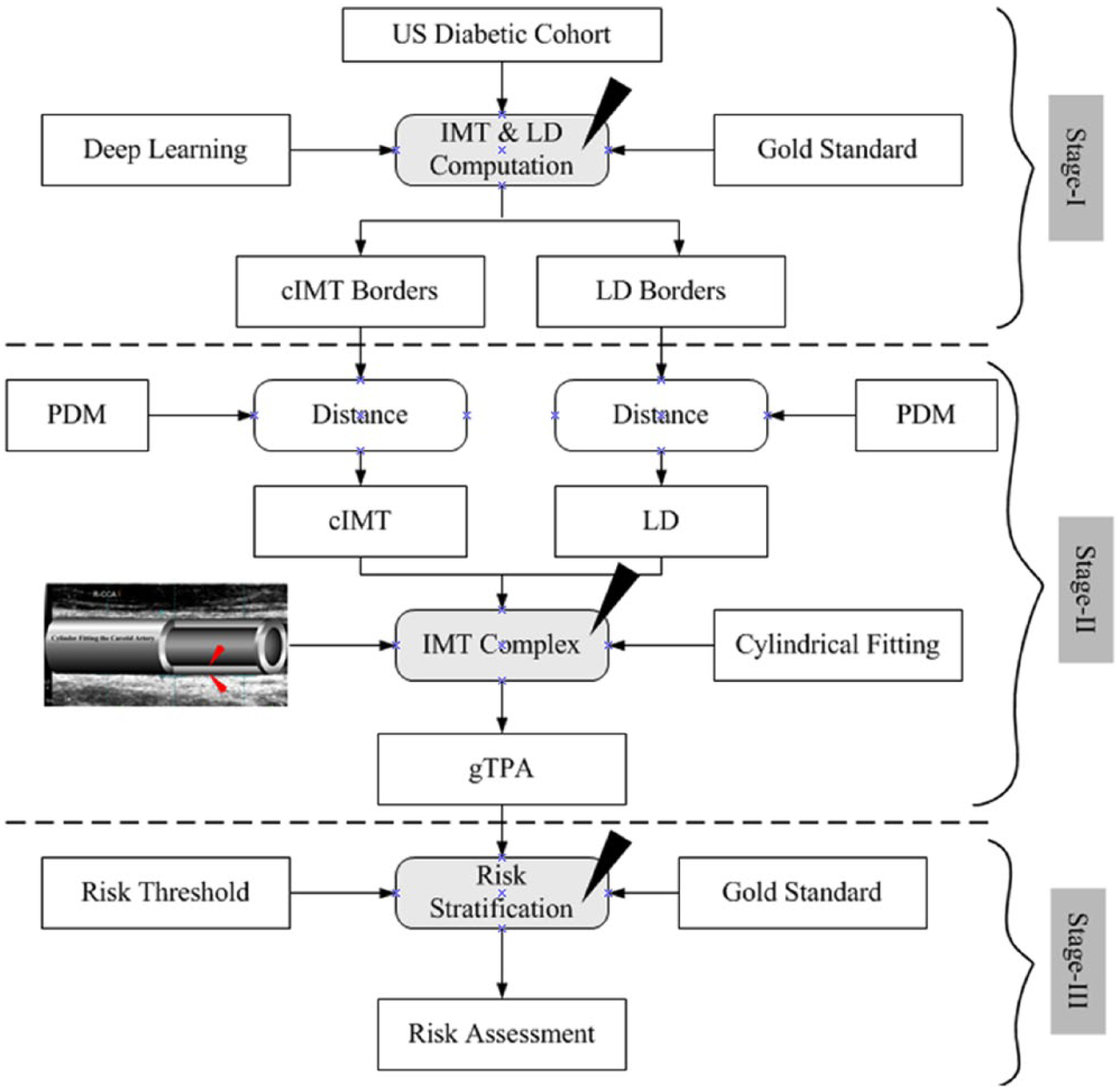
Overall architecture for gTPA and cIMT phenotype measurements and risk stratification.

cIMT and LD Detection Using DL System

In this section, we briefly discuss the concept of how the intelligence is used for deep feature extraction from the grayscale US images and further segment the inner lumen region and outer wall region. The DL system consists of 3 stages: preprocessing, LI and MA region segmentation, and finally LI/MA border detection. The stage 1 requires automatic cropping of the US scans to remove the patient information followed by the process of converting the images to binary along the lines as developed by Suri’s team.⁴⁴ To speed the core of the DL system, we use the previous spirit of Suri’s multiresolution approach for down sampling the carotid scans for cIMT estimation and applications.^22,23,45

The stage 2 is the DL stage consisting of encoder, decoder, and the gold standard. This stage is run 2 times: one for the lumen region extraction and second for the interadventitial outer wall region extraction (Appendix A). When DL is made to run the first time, the gold standard for lumen borders is used for training the DL system, and when used second time, the gold standard for the interadventitial borders is used for the training system. Similarly, the DL system is used 2 times for the test data set for the LD border²⁷ and interadventitial diameter (IAD) borders.⁴⁶ The preprocessed image is then encoded for feature extraction and finally segmentation using decoder along the lines as published by Suri’s team.^27,46 The encoder adapts a 13 layered architecture called VGG16 for feature extraction. This uses the combination of 13 convolutions with 5 max-pooling layers, which is used for downsampling the features from the previous convolution layer. ImageNet is used for computation of the pretrained VGG weights, which are the initialization of the weights during the DL paradigm. Each max-pool layer downsample the features of its previous convolution layer. During the decoding process, the binary output segmentation is performed where the high-level features are computed and transformed by the training weights. The decoding process is performed by the last 3 layers of the VGG16 architecture. Basically, the decoder uses the upsampling layers of Fully Convolutional Network (FCN).⁴⁷ Here, upsampling is performed, while utilizing the skip-connection technique, paving the way to full spatial resolution for semantic segmentation. The cross-entropy loss function was used for spatial segmentation.

The stage 3 consists of calibration process where the machine learning system is used for the correction of raw border estimated from the DL system. This is a linear system leading to final smooth LI/MA border estimation for the far wall. The DL protocol was implemented using cross-validation consisting of 90% training and 10% testing (so-called K10 protocol), where we partition the data set into 10 parts and run the DL system for 10 combinations. For optimization of the results, we took several combination of iterations starting from 4K, 8K, 12K, 16K, and 20K (where K is 1000).⁴⁶

Japanese cohort is used for gTPA calculation. Gold standard data were prepared with the help of sonographer by taking manual readings. Polyline distance method is applied over prepared data set and DL is used for LD measurement (Appendix B). Manual and DL methods are used for cIMT measurement. Finally, we have used Linhart et al²⁴ formula for gTPA calculation. The overall system is demonstrated in Figure 4.

Figure 4.

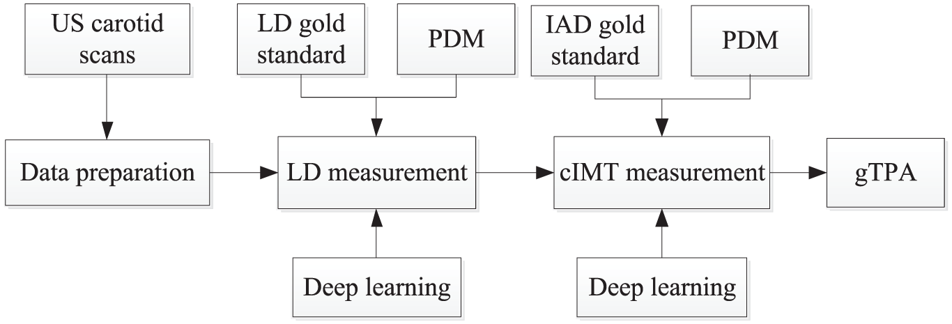
Flow diagram for DL-based LD and cIMT measurements.

Experimental Protocol, Results, and Its Validation

This section consists of the following experimental protocols and its results.

DL system results and visual display of LI and MA interfaces.

Mean value computations for cIMT and gTPA for 2 DL systems.

Relationship of age versus cIMT and gTPA measurements.

Validation of DL systems against the manual readings.

DL System Results and Visual Display of LI and MA Interfaces

A methodology recently developed by Suri’s group²⁷ is used for the computation of LI/MA wall interfaces. The display of LI/MA borders using DL strategy is shown in Figures 5 to 7, respectively, for the low risk, moderate risk, and high risk patients. The LI borders are shown in RED color, MA borders in GREEN color, and YELLOW colors represent the ground truth borders. Figures 5 to 7 represent the sample of low, moderate, and high risk categories of grayscale images of CCA. The corresponding LD, cIMT, and gTPA values are also mentioned.

Figure 5.

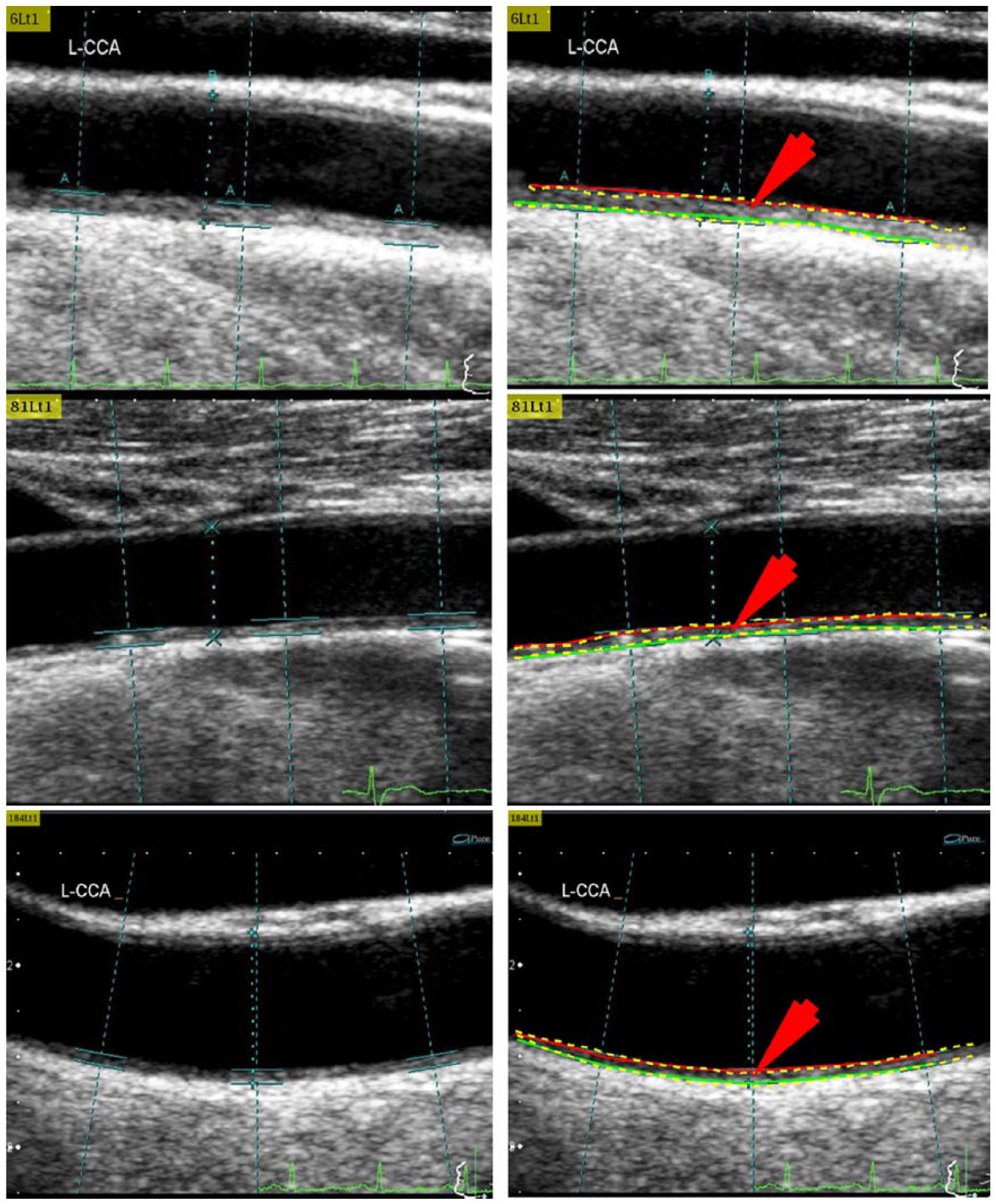
Three examples of low risk category using DL1 system.

Figure 6.

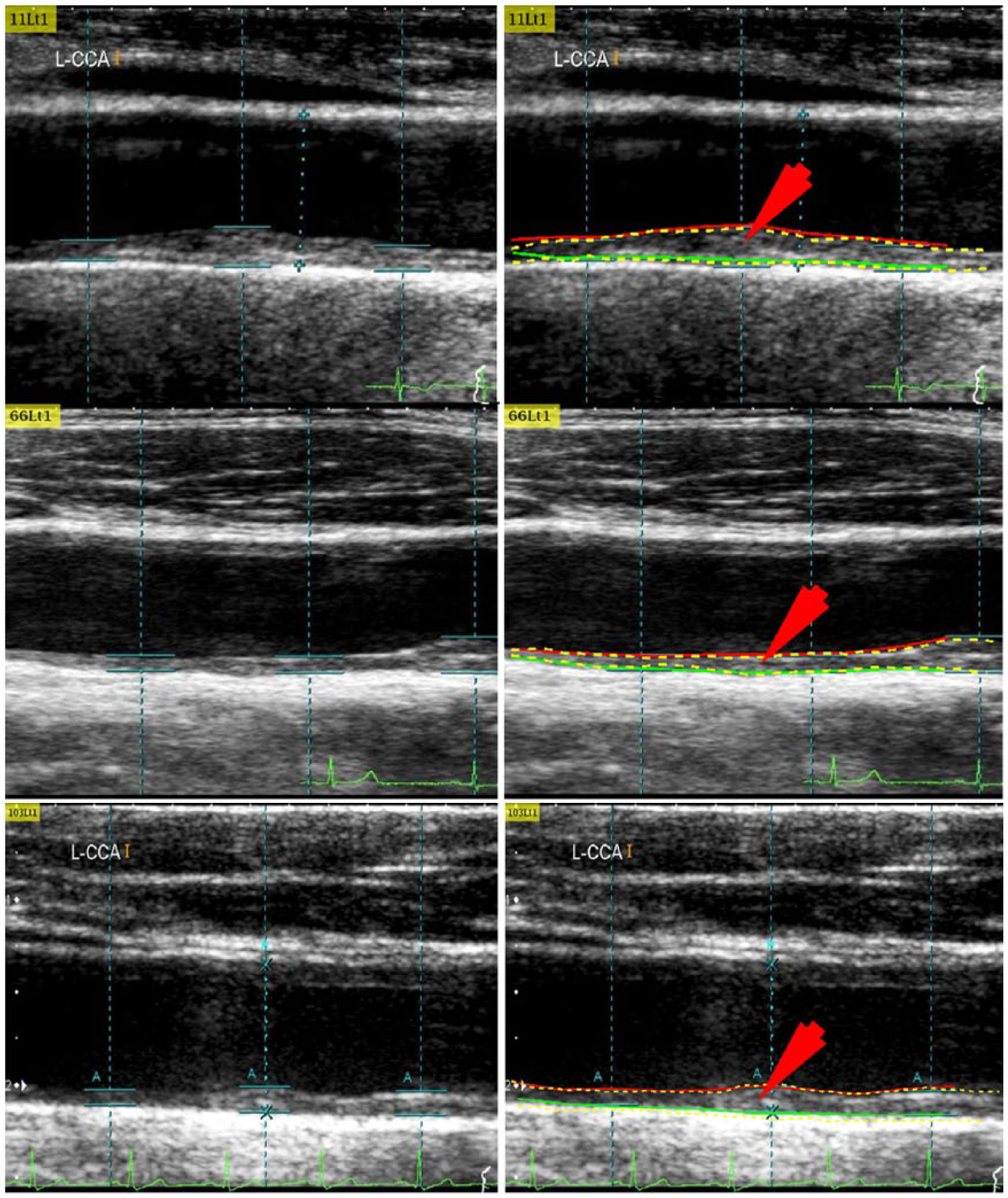
Three examples of moderate risk category using DL1 system.

Figure 7.

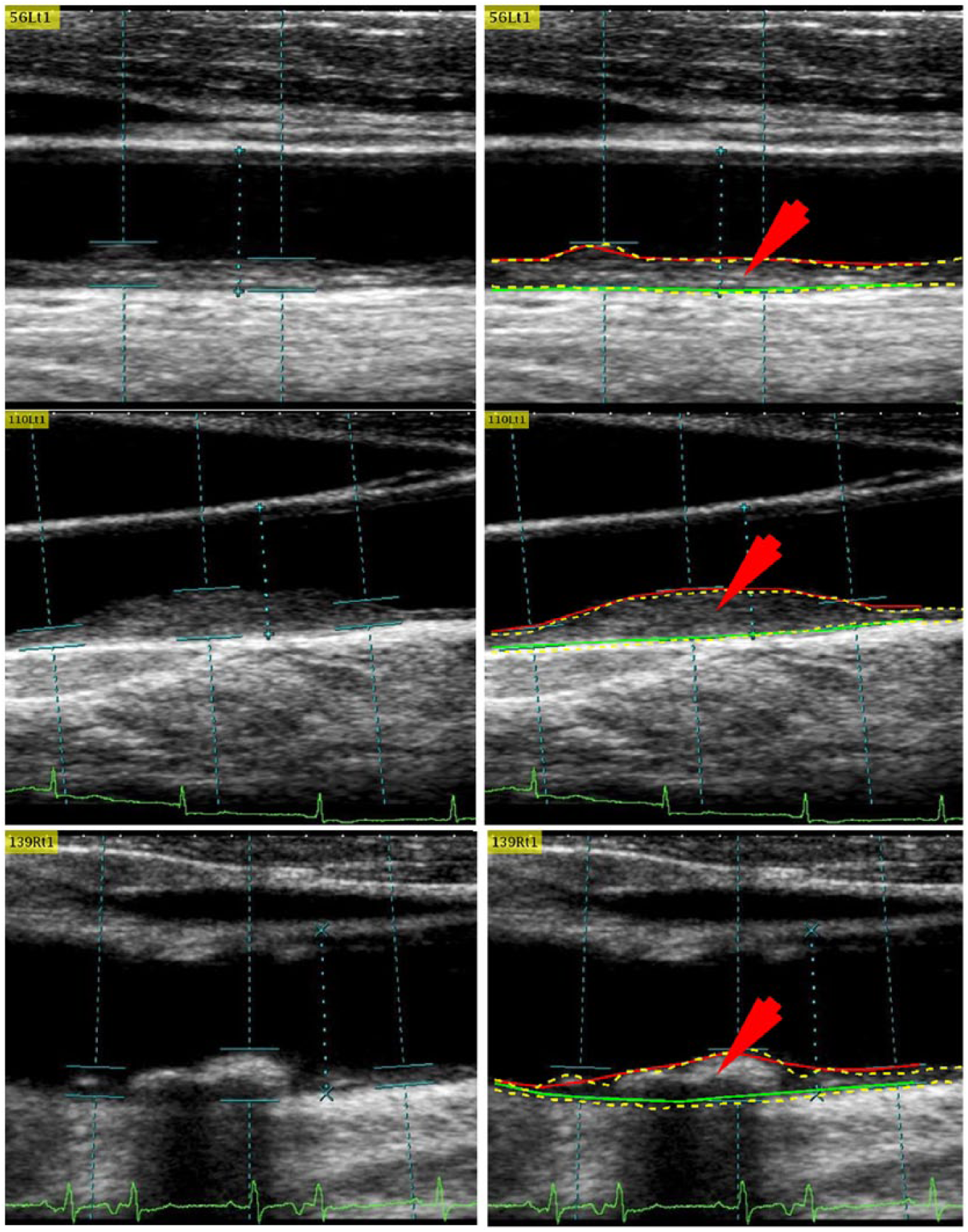
Three examples of high risk category using DL1 system.

Mean Value Computations for cIMT and gTPA for 2 DL Systems

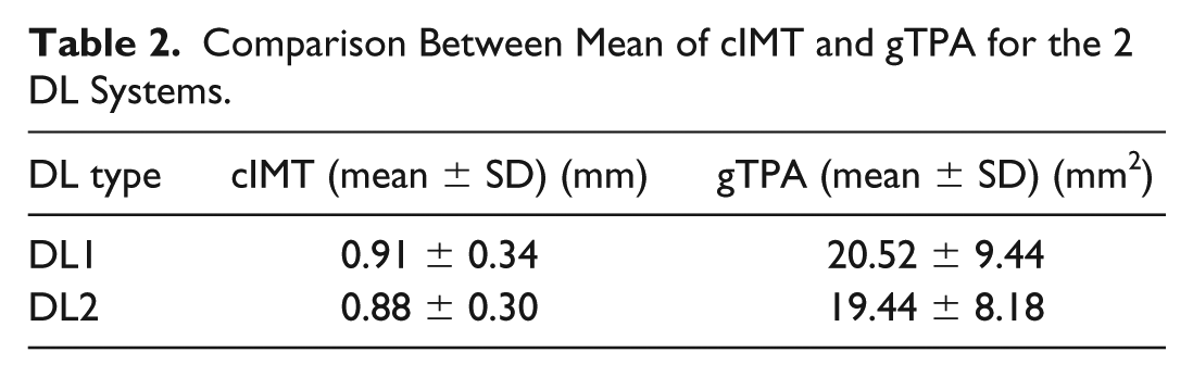
Table 2 shows the mean and standard deviation values of the cIMT and gTPA corresponding to the 2 DL systems.

Table 2.

Comparison Between Mean of cIMT and gTPA for the 2 DL Systems.

DL type	cIMT (mean ± SD) (mm)	gTPA (mean ± SD) (mm²)
DL1	0.91 ± 0.34	20.52 ± 9.44
DL2	0.88 ± 0.30	19.44 ± 8.18

Relationship of Age Versus cIMT/gTPA

The relationship between age versus cIMT and between age versus gTPA is shown in Table 3.

Table 3.

CC of Age (Years) Versus cIMT and gTPA With DL Systems 1 and 2.

SN	Relationship type	CC	P value	Relationship type	CC	P value
1	Age (years) vs cIMT (DL1)	0.1925	<.001	Age (years) vs cIMT (DL2)	0.1868	<.001
2	Age (years) vs cIMT (GT1)	0.1536	<.001	Age (years) vs cIMT (GT2)	0.1415	<.001
3	Age (years) vs gTPA (DL1)	0.2007	<.001	Age (years) vs gTPA (DL2)	0.2038	<.001
4	Age (years) vs gTPA (GT1)	0.1665	<.001	Age (years) vs gTPA (GT2)	0.1554	<.001

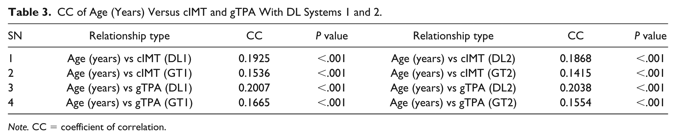
Note. CC = coefficient of correlation.

gTPA was observed to be higher than cIMT for both DL and manual systems. The corresponding plots are as presented in Figures 8 and 9.

Figure 8.

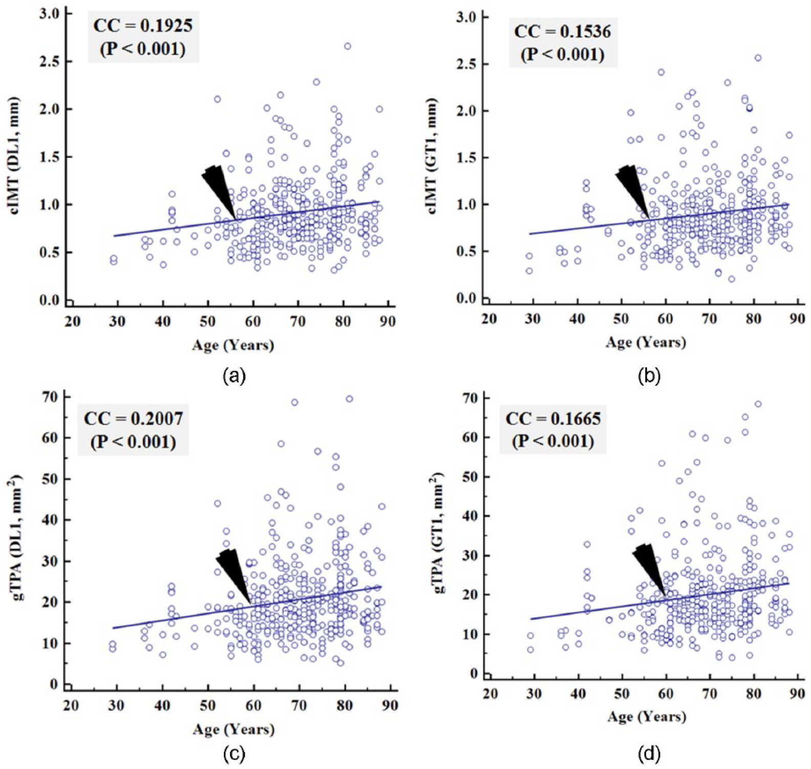
CC plots of age (years) versus cIMT (DL1) and cIMT (GT1) shown in 8(a) and 8(b) and age (years) versus gTPA (DL1) and gTPA (GT1) shown in 8(c) and 8(d) for DL1 system.

Figure 9.

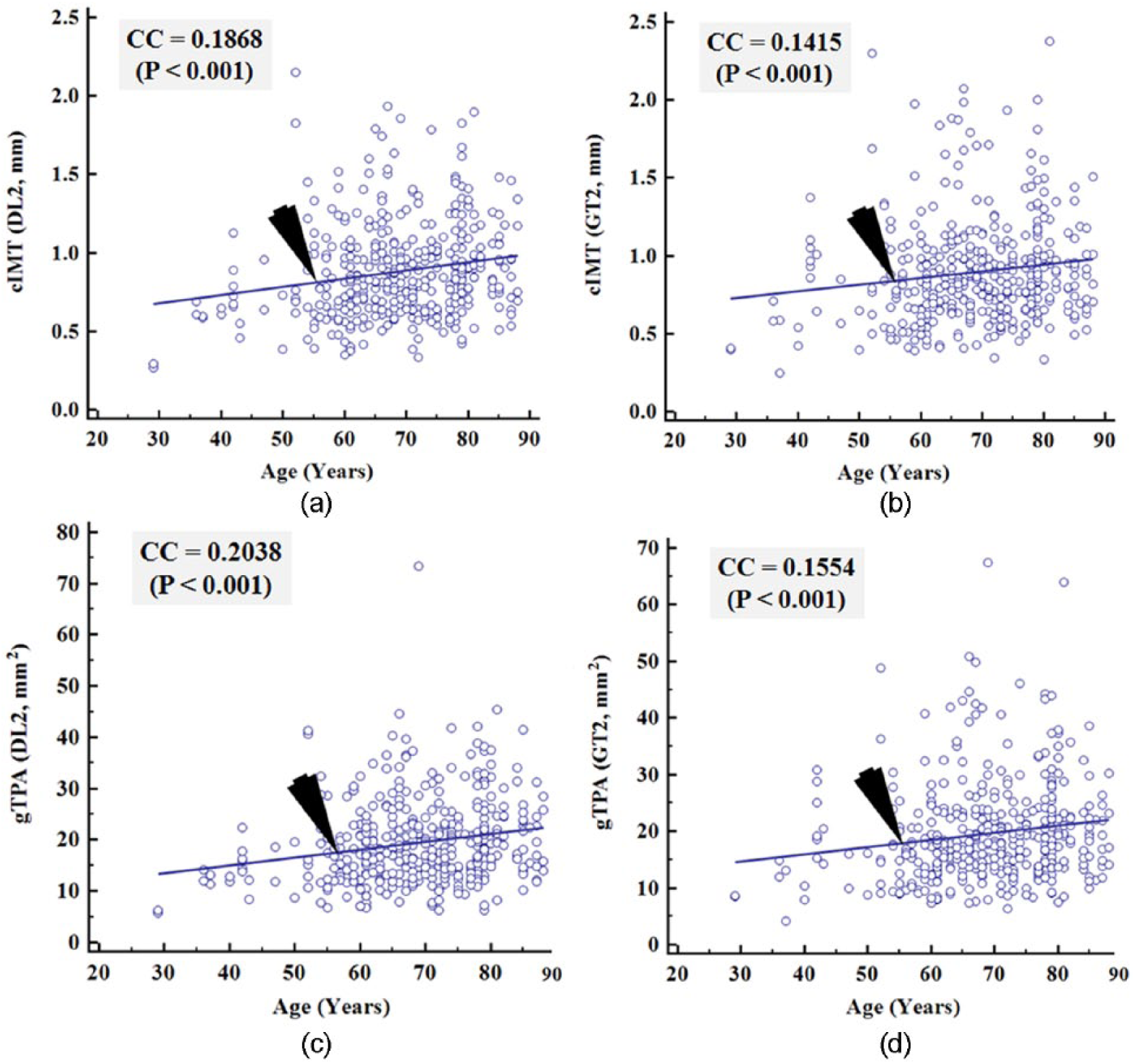
CC plots of age (years) versus cIMT (DL2) and cIMT (GT1) shown in 9(a) and 9(b) and age (years) versus gTPA (DL2) and gTPA (GT2) shown in 9(c) and 9(d) for DL2 system.

Validation

It is important to validate the behavior of gTPA against other wall parameters. This includes cIMT, LD, and IAD derived using DL1 and DL2 frameworks. Furthermore, we need to know how gTPA behaves against the manual (ground truth) readings. If the results between automated system and manual readings tend to show statistical significance, this would signify one step closer to the validation criteria. Sections “gTPA versus cIMT for DL1, GT1, DL2 and GT2” to “gTPA versus IAD for DL1, GT1, DL2, GT2” show the regression plots of the relationships between gTPA and other wall parameters, while the corresponding table is shown in Appendix Table C1.

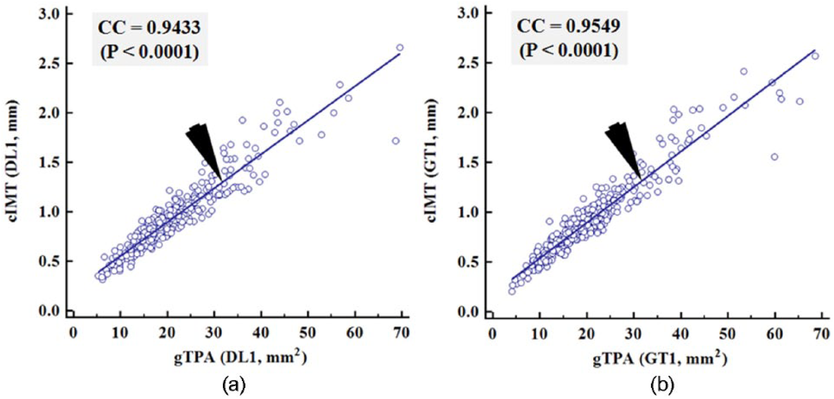
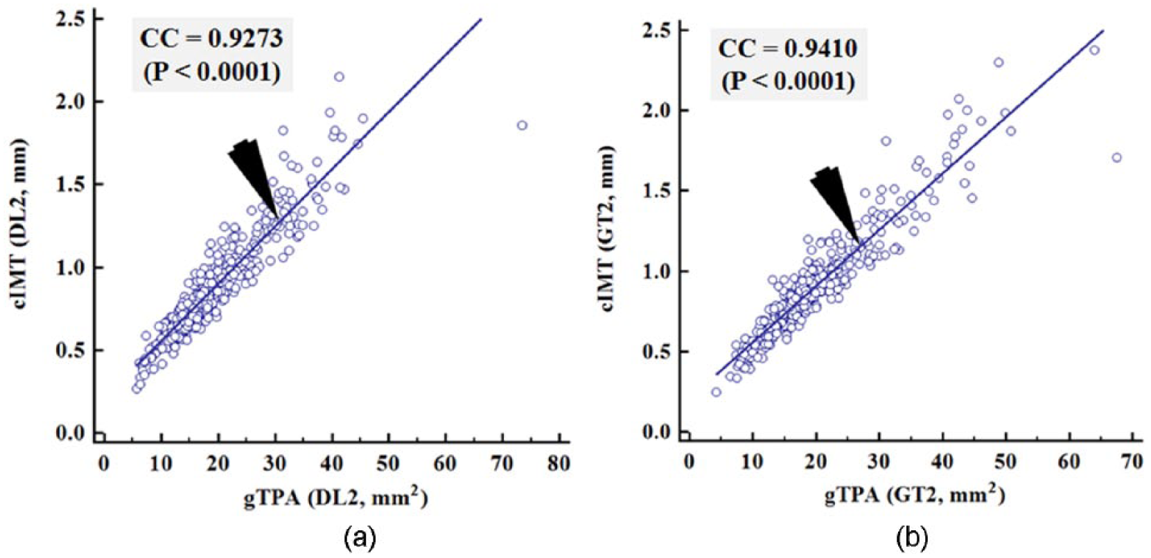
gTPA versus cIMT for DL1, GT1, DL2, and GT2

Figure 10(a) and 10(b) shows the CC plots of gTPA (DL1) versus cIMT (DL1) and gTPA (GT1) versus cIMT (GT1). The CC value for DL system was 0.94 (P value < .001), while for the manual reading, it was 0.95 (P value < .001). This clearly shows the consistent behavior of DL with the doctor’s manual readings. Above results prove our assumption that if the CC values are close to each other, and if the behavior is linear, then the DL can be considered to be validated. A similar pattern was observed between gTPA (DL2) versus cIMT (DL2) (see Figure 11(a)) and gTPA (GT2) versus cIMT (GT2) (see Figure11 (b)) leading to CC values of 0.92 (P value < .001) and 0.94 (P value < .001). Above results prove the consistency of DL1 and DL2 systems.

Figure 10.

Correlation plots of gTPA (DL1) versus cIMT (DL1) and gTPA (manual 1) versus cIMT (manual 1) based system. Manual implies GT.

Figure 11.

Correlation plots of gTPA (DL2) versus cIMT (DL2) and gTPA (manual 2) versus cIMT (manual 2) based system. Manual implies GT.

gTPA versus LD for DL1, GT1, DL2, GT2

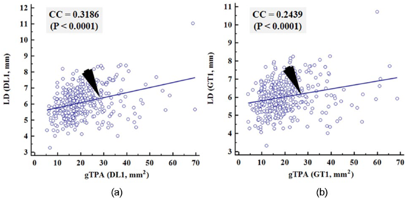
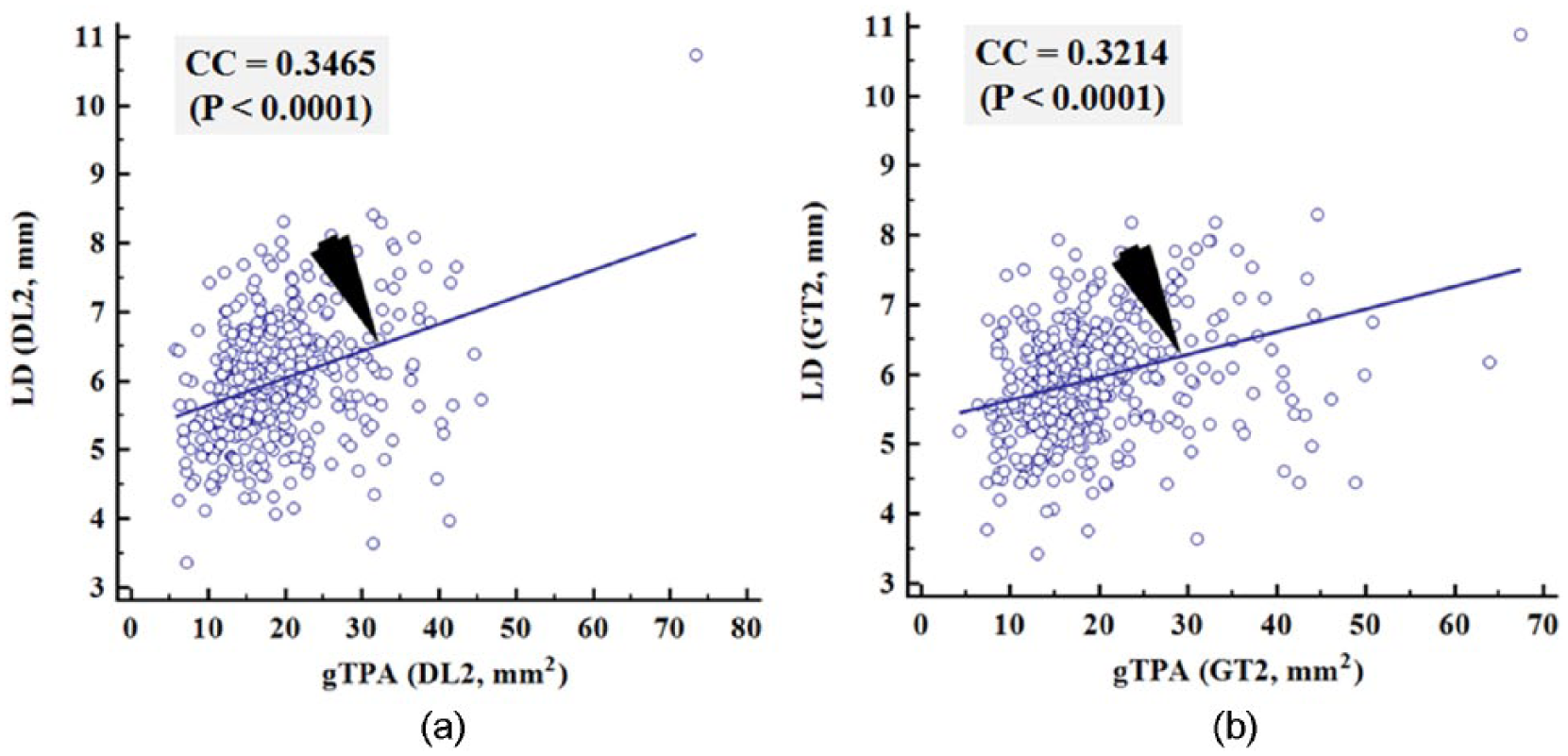
We further validated the relationship between gTPA and LD for DL1 against GT1, and DL2 against GT2. This can be seen in Figure 12(a), which shows the correlation plots of gTPA (DL1) versus LD (DL1) using DL1 system, while Figure 12(b) shows the relationship between gTPA (GT1) versus LD (GT1). Note that the CC was 0.31 (P value < .001) and 0.24 (P value < .001) for DL1 and GT1 systems, respectively. A similar pattern was observed for gTPA (DL2) versus LD (DL2) (see Figure 13(a)) and gTPA (GT2) versus LD (GT2) (see Figure 13(b)) leading to CC values of 0.34 (P value < .001) and 0.32 (P value < .001). This proves our assumption that if the CC values are close to each other, and the behavior is linear, then the DL systems can be considered to be validated. Note that the CC between gTPA versus LD is not as strong as gTPA versus cIMT, which is obvious. This is due to the reason that as cIMT increases, TPA must increase and as LD increases (heading to normal), the gTPA will be moderate or low. This further validates the stability of DL systems.

Figure 12.

Correlation plots of gTPA (DL1) versus LD (DL1) and gTPA (manual 1) versus LD (manual 1) based system.

Figure 13.

Correlation plots of gTPA (DL2) versus LD (DL2) and gTPA (manual 2) versus LD (manual 2) based system. Manual implies GT.

gTPA versus IAD for DL1, GT1, DL2, GT2

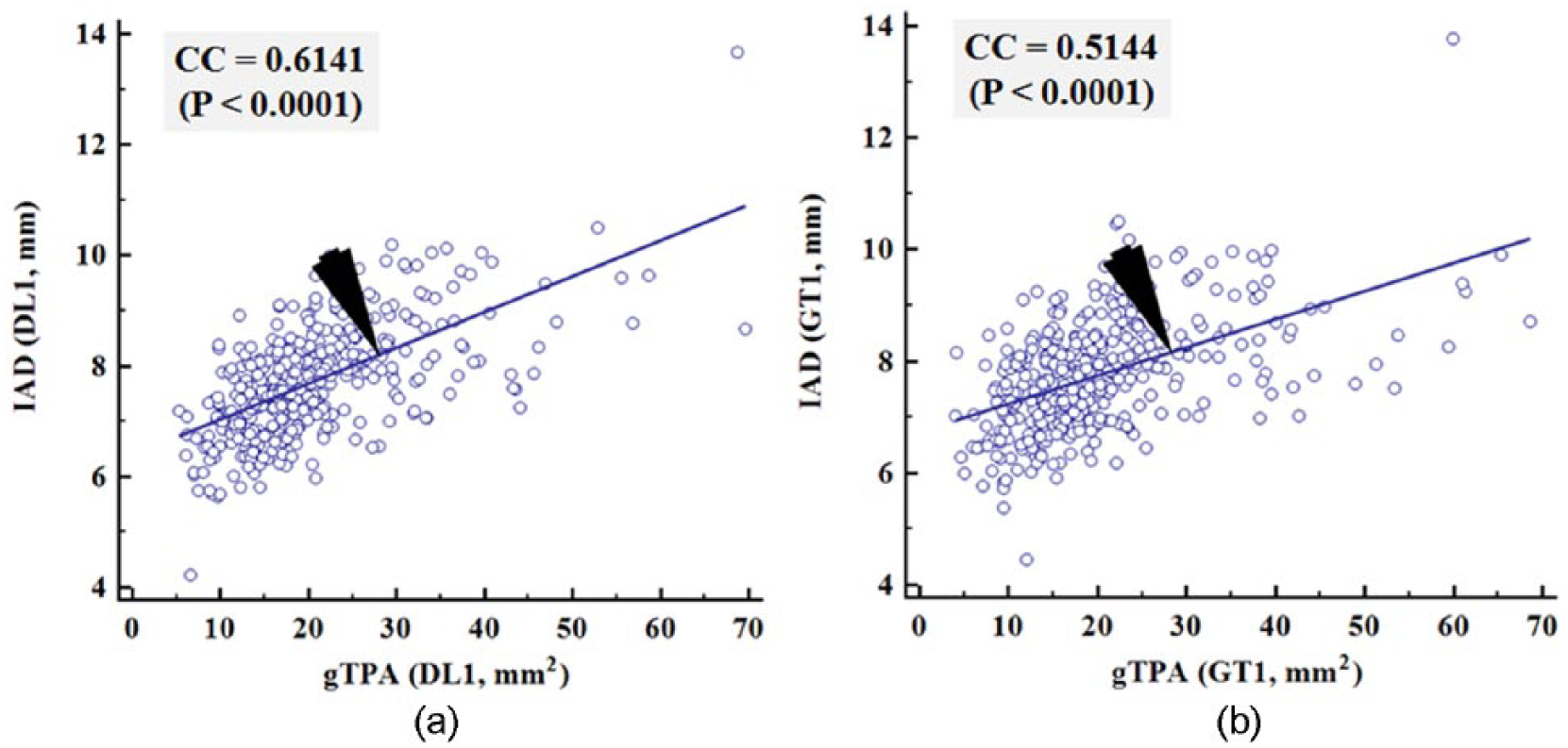
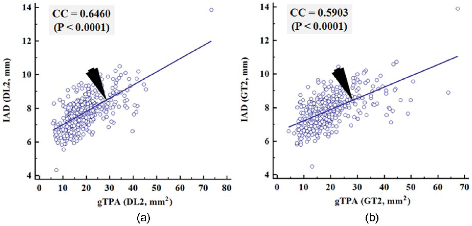
We further validate the relationship between gTPA and IAD for DL1 against GT1 and DL2 against GT2. This can be seen in Figure 14(a), which shows the correlation plots of gTPA (DL1) versus IAD (DL1) based system, while Figure 14(b) shows the relationship between gTPA (GT1) versus IAD (GT1). Note that the CC is 0.61 (P value < .001) and 0.51 (P value < .001), respectively. A similar pattern was observed for gTPA (DL2) versus IAD (DL2) (see Figure 15(a)) and gTPA (GT2) versus IAD (GT2) (see Figure 15(b)) leading to CC values of 0.64 (P value < .001) and 0.59 (P value < .001). This clearly shows both DL1 and DL2 systems had same behavior with respect to manual readings. These results further prove our assumption that if the CC values are reasonably close to each other, and the behavior is linear, then the DL can be considered to be validated.

Figure 14.

Correlation plots of gTPA (DL1) versus IAD (DL1) and gTPA (manual 1) versus IAD (manual 1) based system.

Figure 15.

Correlation plots of gTPA (DL2) versus IAD (DL2) and gTPA (manual 2) versus IAD (manual 2) based system. Manual implies GT.

Bland-Altman plots

The Bland-Altman plots of the average of gTPA (DL1) and cIMT (DL1) and average of gTPA (GT1) and cIMT (GT1) for DL1 and GT1 system, respectively, are shown in Figure 16. Similar pattern was also shown in Figure 17 and represents average of gTPA (DL2) versus cIMT (DL2) and average of gTPA (GT2) versus cIMT (GT2) for DL2 and GT2 system, respectively.

Figure 16.

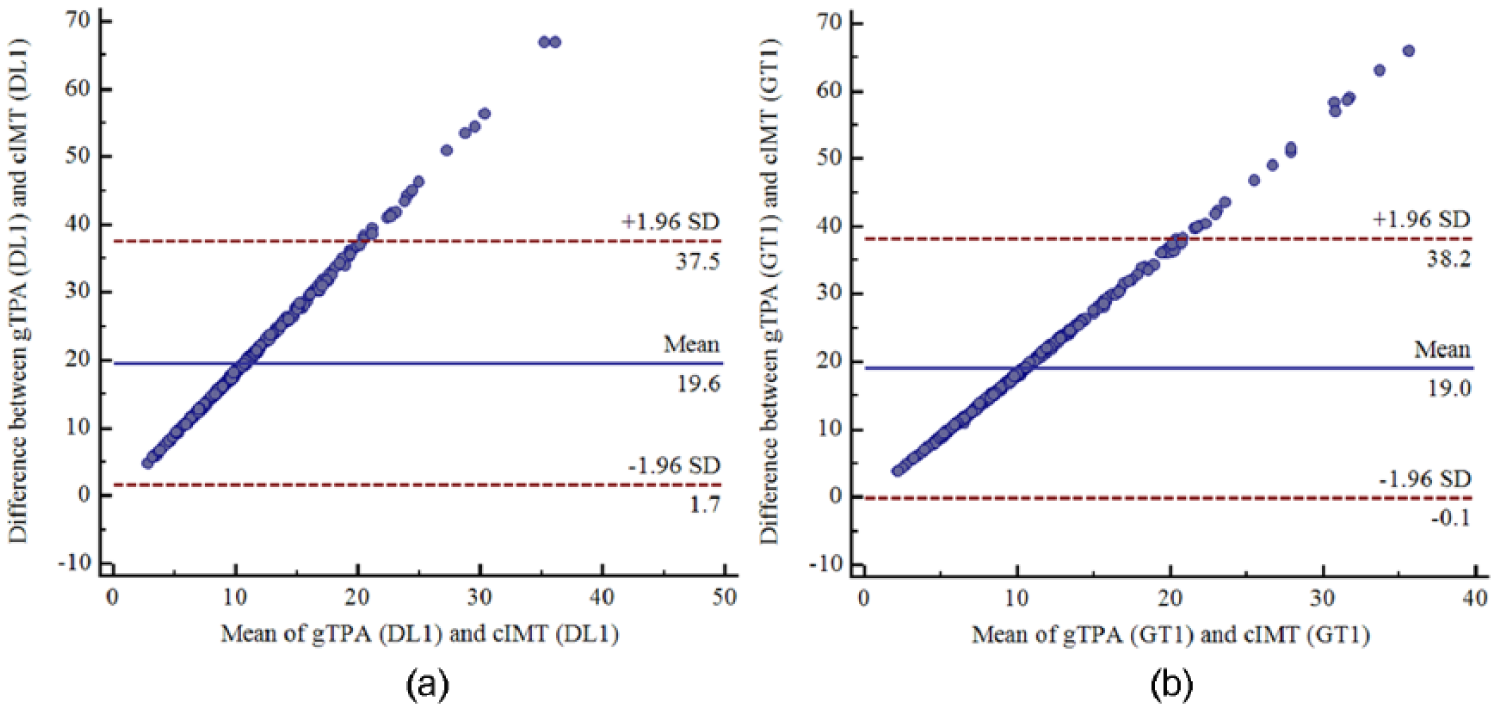
Bland-Altman plots of mean of gTPA (DL1) versus cIMT (DL1) and mean of gTPA (GT1) versus cIMT (GT1).

Figure 17.

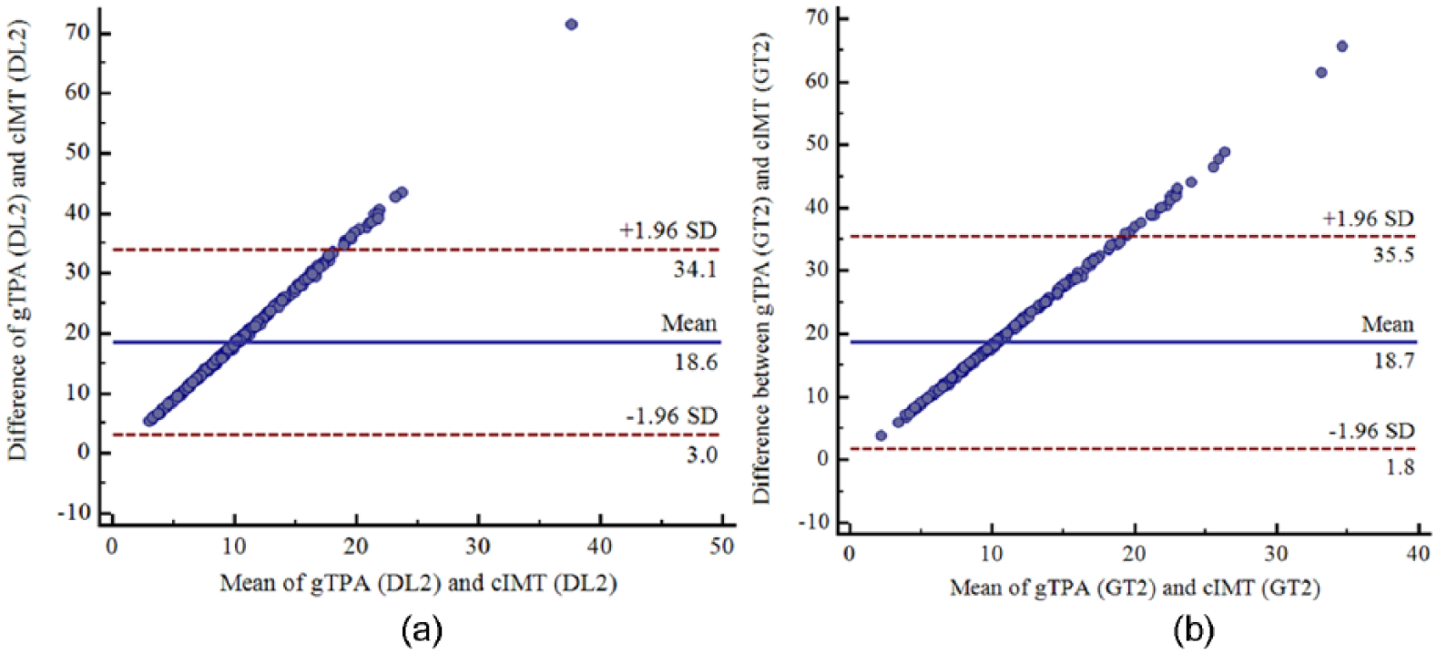
Bland-Altman plots of mean of gTPA (DL2) versus cIMT (DL2) and mean of gTPA (GT2) versus cIMT (GT2).

The Bland-Altman plot or difference plot is used to compare the 2 measurement techniques. It is a graphical method, which shows the differences and plots the averages of the 2 techniques. Finally, the mean differences are plotted against the 2 methods. The limit of agreement defines the mean differences and ±1.96 times the standard deviation (SD) of the differences. It is a well-known measurement technique, which shows the systematic biasing between measurements and informs us how far the 2 methods are likely to be. When we are comparing or assessing methods repeatability, it is important to calculate confidence intervals for 95% limits of agreement.

Statistical Tests and 10-Year Risk Analysis

Risk Analysis

Receiver operating characteristic (ROC) is a measure of performance validation of any technique as it captures all the record variation at every possible cutoff. Area under the curve value shows the accuracy of the performance measure. For ROC analysis, the cohort data are divided into 3 risk classes: low risk, moderate risk, and high risk patients using 2 cutoffs. For gTPA, the cutoffs were 20 mm² and 40 mm². For cIMT, the cutoffs were 0.6 mm and 0.9 mm: low risk (0 mm to less than 0.6 mm), moderate risk (greater and equal to 0.6 mm and less than 0.9 mm), and high risk (greater and equal to 0.9 mm). Same thresholds were considered while evaluating the manual readings. The plots for both DL systems and manual systems are shown in Figure 18(a) and Figure 18(b). From the plots, it can be observed that gTPA performs better than cIMT for both DL and manual systems.

Figure 18.

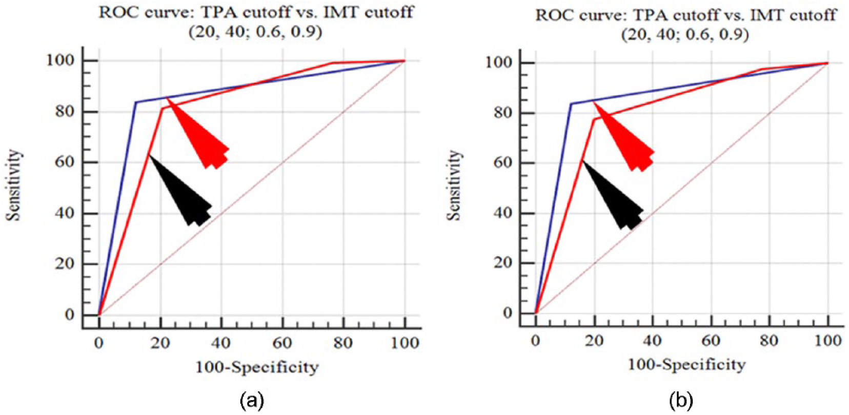
ROC plot comparison between gTPA and cIMT for (a) DL1 and (b) GT1.

Statistical Tests

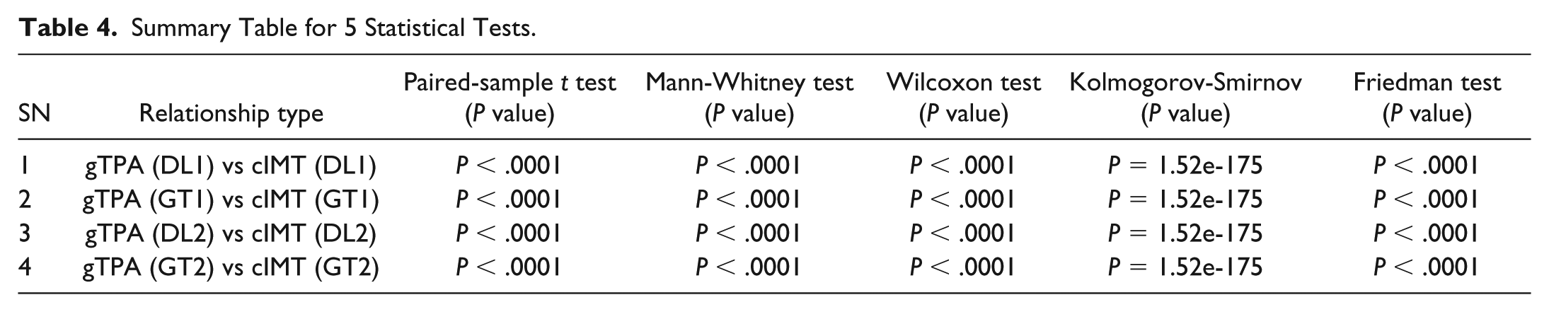
All the 5 statistical test results (paired-sample t test, Mann-Whitney test, Wilcoxon test, Kolmogorov-Smirnov test, and Friedman test) are shown in Table 4. The P values of the results confirm that the paired samples qualify the test successfully. The results of DL-based system with respect to GT1 and GT2 have been analyzed and tested using paired-sample t test, Mann-Whitney test, and Wilcoxon test whose corresponding box-plots are shown in Figure 19.

Table 4.

Summary Table for 5 Statistical Tests.

SN	Relationship type	Paired-sample t test(P value)	Mann-Whitney test(P value)	Wilcoxon test(P value)	Kolmogorov-Smirnov(P value)	Friedman test(P value)
1	gTPA (DL1) vs cIMT (DL1)	P < .0001	P < .0001	P < .0001	P = 1.52e-175	P < .0001
2	gTPA (GT1) vs cIMT (GT1)	P < .0001	P < .0001	P < .0001	P = 1.52e-175	P < .0001
3	gTPA (DL2) vs cIMT (DL2)	P < .0001	P < .0001	P < .0001	P = 1.52e-175	P < .0001
4	gTPA (GT2) vs cIMT (GT2)	P < .0001	P < .0001	P < .0001	P = 1.52e-175	P < .0001

Figure 19.

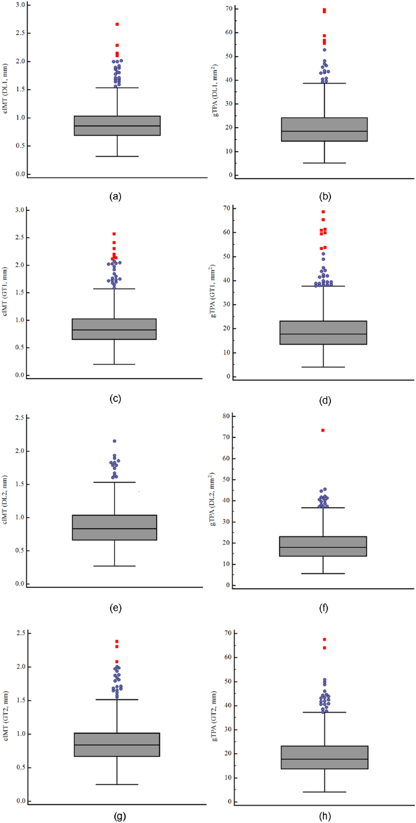
Box plots of cIMT and gTPA for both DL1 and DL2.

The corresponding P values for paired-sample t test corresponding to gTPA and cIMT with reference to both DL systems and its ground truth values are observed to be less than .0001, This proves that the results are statistically significant for all the combinations; results are shown in Appendix D (Tables D1, D5, D9, and D13). The P values for Mann-Whitney test for DL1 and DL2 with reference to GT1 and GT2 corresponding to gTPA and cIMT are less than .0001. This proved that both the results are statistically significant and are as shown in Appendix D (Tables D2, D6, D10, and D14). The P values for Wilcoxon test for DL1 and DL2 with reference to GT1 and GT2 corresponding to gTPA and cIMT are less than .0001. This proved that both the results are statistically significant and are as shown in Appendix D (Tables D3, D7, D11, and D15). We have performed Kolmogorov-Smirnov test for DL1 and DL2 and results are significant in terms of their P values. The P values with respect to DL1 and DL2 were below .0001. Furthermore, we performed Friedman tests for DL1 and DL2 and their corresponding results are shown in Appendix D (Tables D4, D8, D12, and D16). The P values corresponding to DL1 and DL2 are below .0001, therefore rejecting the null hypothesis that the data taken from same distribution cannot be retained for DL1 and DL2.

Ten-Year Risk Assessment

Risk assessment is a mechanism through which we can identify the CVD risk based on the cIMT thickness and gTPA. Here, we considered 10-year risk for all the patients. The cohort consists of both male and female categories, so the risk is calculated as per following equations 4 to 7:

\begin{array}{l} cIMT (10-year, men) = cIMT (current, men) + \\ Projection Rate (men) \times 10, \end{array}

(4)

\begin{array}{l} cIMT (10-year, women) = cIMT (current, women) + \\ Projection Rate (women) \times 10, \end{array}

(5)

\begin{array}{l} gTPA (10-year, men) = gTPA (current, men) + \\ Projection Rate (men) \times 10, \end{array}

(6)

\begin{array}{l} gTPA (10-year, women) = gTPA (current, women) + \\ Projection Rate (women) \times 10, \end{array}

(7)

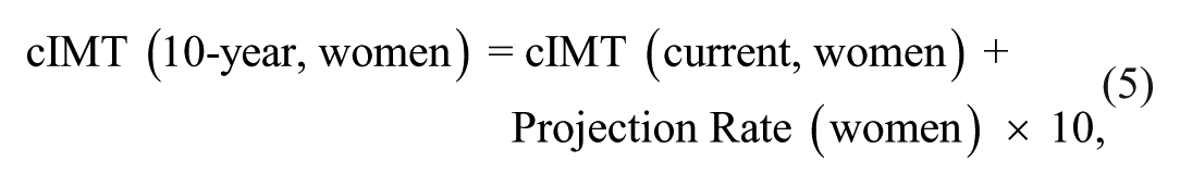
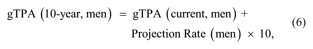
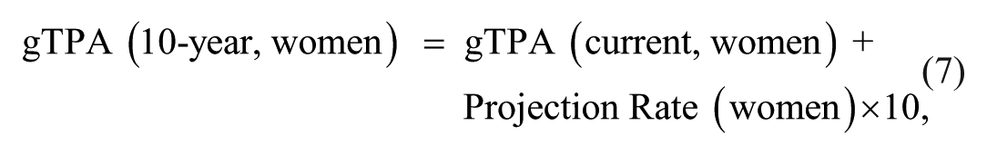
where the projection rate for the Japanese men and women are 0.03 mm/year and 0.02 mm/year, respectively. Our aim is to design a linear model for computing the 10-year risk due to age.

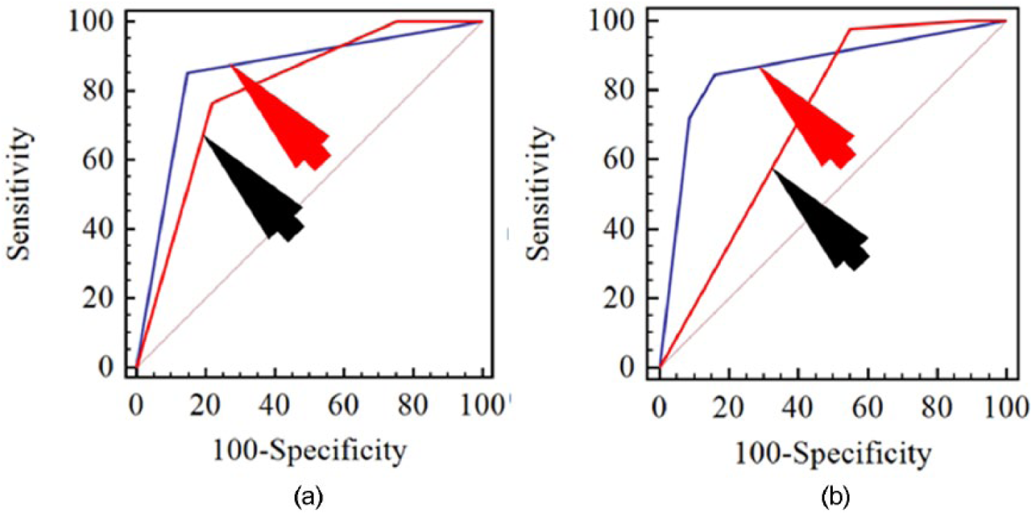
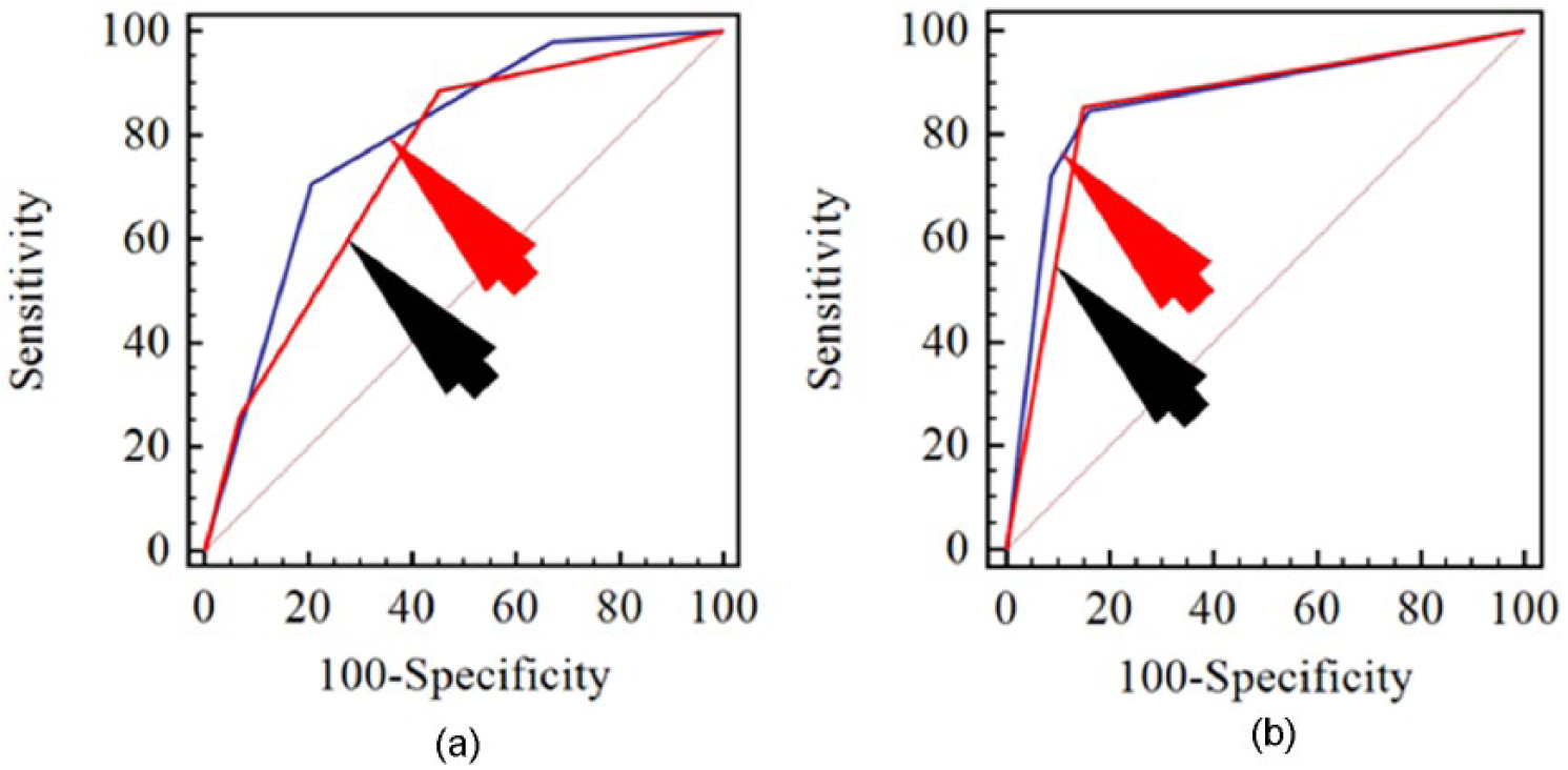
Note that the our model does not take into consideration CCVR factors such as the effect of diabetes, body mass index (BMI), low-density lipoproteins (LDL), and systolic blood pressure (SBP) due to its simplicity and scope of work. The current versus 10-year risk corresponding to cIMT and gTPA for both DL systems is shown in Figures 20 and 21. The corresponding AUC summary is shown in Table 5.

Table 5.

Current Risk Versus 10-Year Risk.

Type of plot (DL system 1)	AUC (before)	AUC (after)	Type of plot (DL system 2)	AUC (before)	AUC (after)
cIMT (DL1) vs cIMT (GT1)	0.745	0.792	cIMT (DL2) vs cIMT (GT2)	0.764	0.819
gTPA (DL1) vs gTPA (GT1)	0.852	0.864	gTPA (DL2) vs gTPA (GT2)	0.860	0.870

Figure 20.

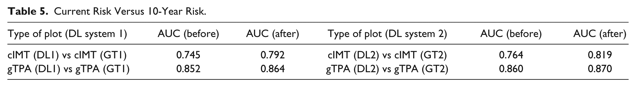
ROC plots of cIMT versus gTPA. (a) Current cIMT risk (red) versus current gTPA risk (blue). (b) 10-year cIMT (red) versus 10-year gTPA (blue).

Figure 21.

ROC plots of current risks versus 10-year risks. (a) Current cIMT risk (red) versus 10-year cIMT risk (blue), (b) current gTPA risk (red) versus 10-year gTPA risk (blue).

Table 5 showed that current gTPA is higher than current cIMT and gTPA10 is better than cIMT10, which proves our assumption that gTPA is a strong clinical biomarker for stroke risk and can be adapted for risk assessment. The AUC for gTPA showed an improvement over cIMT by 14.36% and 12.57% for DL1 and DL2, respectively. The corresponding 10-year risk improvements were 9.09% and 6.26%.

Discussion

The study presented a cylindrical-based model for the automated computation of gTPA, given the cIMT and LD. An intelligence-based technique²⁷ was employed for computing the cIMT and LD. We demonstrated that gTPA is an equally strong biomarker as cIMT for risk assessment. The results showed a high CC between gTPA and cIMT using DL and manual, 0.92 (P < .001) and 0.94 (P < .001), respectively. Furthermore, by using 2 cutoffs, leading to low, moderate, and high risk assessment system, the AUC for cIMT and gTPA was 0.76 (P < .001) and 0.85 (P < .001) using DL1 and 0.76 (P < .001) and 0.86 (P < .001) using DL2, respectively. The study further demonstrates that gTPA is more strongly associated with age compared with cIMT. Note that our model was only applicable to CCA for its subclinical atherosclerosis modeling, unlike bulb or ICA.

Benchmarking

There are several similarities between our study and the work done by others. This can be seen from Table 6; we can observe that most of the previously published work used “manual” criteria for gTPA measurement while current study adapted automated morphological-based gTPA measurement. Furthermore, the current study used intelligence-based criteria for cIMT and LD for detection.

Table 6.

Benchmarking Table.

C1	C2	C3	C4	C5	C6	C7	C8	C9	C10	C11	C12	C13	C14	C15
SN	Author & year	PS	Class	HT	HbA1c(mg/dL)	LDL-C	BMI(kg/m²)	Age(mean)	TPA, mm² (2 cutoff)	Type	DM (%)	TPA^a Tech.	Male/Female	Smoking(%)
R1	Spence et. al (2008)	876	2	—	—	—	—	53.4 ± 12	38	M	6.7	mTPA (w)	463 (Ma) 413 (F)	For-39.6 Cu-11.5
R2	Matheisen et. al (2012)	2743	2	—	—	—	25.85 ± 3.5	56.2 ± 9.64	6.08	L	1.40	mTPA (wp)	1307 (Ma) 1436 (F)	Cu-27.7
R3	Matheisen et. al (2013)	4194^a	2	—	—	—	26.6 ± 3.9	61.2 ± 9.8	9.85 ± 16.2	L	—	mTPA (w)	1994 (Ma) 2200 (F)	—
R4	Rundek et. al (2013)	1327^b	3 (EL, I, ED)	71%	—	129 ± 34	28 ± 5	66 ± 9	9.1 & 21.5	LM	20	mTPA (wp)	544 (Ma) 783 (F)	Ne-48, For-37, Cu-15
R5	Rundek et. al (2015)	1356^b	2	—	—	—	—	<70 (744) 70 + (612)	20.3	LM	N81 Y19	mTPA (w)	540 (Ma) 816 (F)	No-48 Yes-52
R6	Spence et. al (2016)	2035	3 (LR, MR, HR)	35%	—	—	—	59 ± 0.2	33.0 & 80.4	MH	14	mTPA (wp)	1175 (Ma) 860 (F)	—
R7	Spence et. al (2017)	2447	2	—	—	<1.8	27.61 ± 5.0	63.59 ± 13.4	113.33 ± 121.5 129.56 ± 134.3	H	16.7	mTPA (wp)	1413 (Ma) 1174 (F)	16.24 ± 19.6
R8	Adams et. al (2017)	5144	4	—	—	3.8 ± 1.0		51.5 ± 9.5	25 & 75	M	—	mTPA (wp)	3073 (Ma)2071 (F)	Cu-23.8
R9	Adams et. al (2018)	8008	6 (Ty1, Ty2a &b, Ty3, Ty4a & b)	—	—	158 ± 39	27.96 ± 4.2	54 ± 6	70 & 120	H	8.4	mTPA (wp)	—	Cu-43.2
R10	Proposed(2018)	204	3 (LR, MR, HR)	—	5.8 ± 1.0	101.1 ± 31.5		68.9 ± 11.0	20 & 40	M	—	gTPA	157 (Ma)47 (F)	—

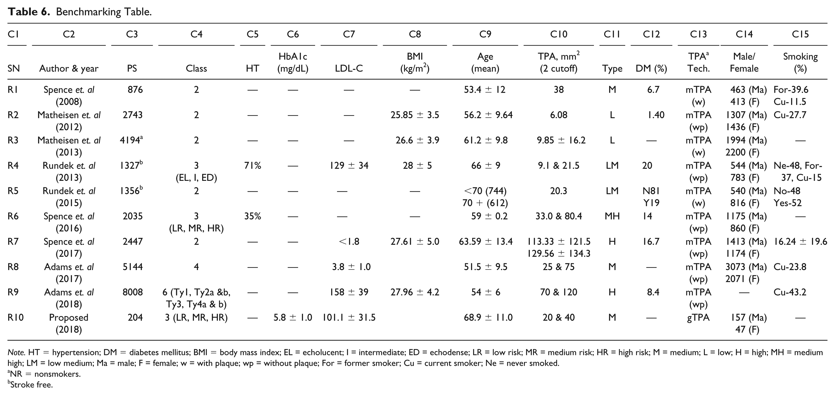
Note. HT = hypertension; DM = diabetes mellitus; BMI = body mass index; EL = echolucent; I = intermediate; ED = echodense; LR = low risk; MR = medium risk; HR = high risk; M = medium; L = low; H = high; MH = medium high; LM = low medium; Ma = male; F = female; w = with plaque; wp = without plaque; For = former smoker; Cu = current smoker; Ne = never smoked.

NR = nonsmokers.

Stroke free.

The work of Spence et al^14,43 has been prominent for TPA computation. The demographics of the study consisted of 1686 patients with mean age (56.95 years), mean hypertension range (650 mm Hg), BMI range (27.4 kg/m²), mean diabetes mellitus (8.9 mg/dL), mean pack years of smoking (12.6 years), and percentage of male and female (53% and 47%). The study identified low and moderate category of carotid plaque for early state cardiovascular risk detection with cutoffs 4.4 mm² and 21.2 mm².

Two years later, the same group¹⁵ again published a study consisting of 1821 patients with mean age of 57.2 ± 14.6 years, mean LDL-C of 3.2 ± 1.13 mg/dl, BMI range of 27.4 kg/m², and 963 males and 858 females for TPA calculation. The 2 mean TPA cutoffs were 87 mm² and 106 mm². The study had an objective of identification of carotid plaque for cardiovascular risk. For the moderate type of risk stratification, Spence and Solo⁴⁸ took 876 patients with mean age of 53.4 ± 12.0 years with an average 6.7% diabetes mellitus cases, out of which 11.5% were smokers. This study considered 463 male and 413 females. The mean TPA cutoff was 38 mm².

Mathiesen et al¹⁷ proposed a mechanism for identifying gTPA. The demographics consisted of a total 6580 patients with mean age 60.2 ± 10.2 years. The patients were categorized into low risk of plaque burden by considering gTPA cutoff value of 3.9 ± 2.2 mm². This study had quite low cutoff, partially due to attributing factor due to low percentage (3.22%) of diabetes mellitus patients. Mathiesen et al¹⁸ again presented a study of 2743 patients having an average gTPA cutoff of 6 mm². The patient demographics consisted of an average age of 56.2 ± 9.65 years and average BMI of 25.85 ± 3.5 kg/m². Mathiesen et al¹⁹ considered 4194 nonsmoker patients in the study for identifying the low risk associated with plaque burden. Their gTPA cutoff for the low risk category was 13 mm². The difference in cutoff can be attributed to factors like lower age group (61.2 ± 9.8 years), nonsmokers, and higher female (2200) compared with male (1994) patient population.

Alsulaimani et al¹⁶ presented a study consisting of cohort having 71% hypertensive, high HbA1c (129 ± 34 mmol/mol), and 20% diabetes patients with an average age of 66 ± 9 years. Their low risk cutoff was 9 mm². This can be attributed to lower female participants in the cohort. The study showed that females (783) had a lower plaque burden compared with male (544) candidates. Rundek et al⁴⁹ further presented a study where 45% of the cohort consisted of high age group (>70 years) and the TPA cutoff was 20 mm², stratifying the risk into low risk and moderate risk.

Spence et al⁴³ considered a cutoff which was twice the cutoff of our current study. The study consisted of cohort (2035 patients) with 35% hypertensive, 37% with higher SBP, and 14% were diabetic. The study took an average of 16 mm², 33 mm², and 80 mm² cutoff points for risk stratification into low risk, moderate risk, and high risk patients. Our current study took 2 cutoffs for gTPA as 20 mm² and 40 mm², which is closer to Spence’s study.⁴³ The slight difference between our cutoff and Spence’s cutoff lies due to the demographic factors like hypertension, diabetes, and hypercholesterolemia.

Spence and Solo⁴⁸ showed that plaque burden (TPA) is a good predictor of CVD. The study showed that the low level of LDL-C did not result in plaque burden and even patients having low LDL-C showed resistance to atherosclerosis. A study was published by Suri and his team demonstrating 34% more plaque in bulb compared with CCA.³⁴ The study¹⁵ found substantial proportion of high risk patient with plaque progression despite low level of LDL-C. The study considered higher male percentage with 16% diabetic, higher BMI, and higher cholesterol patients yielding higher TPA.

Recently, Romanens et al²⁰ presented an extensive study for detection of subclinical atherosclerosis by lowering the risk thresholds. The study showed patients taken from younger age group (51.5 ± 9 years) for detection of moderate and low risk of plaque burden using morphological TPA calculation method. Their cutoffs for low and moderate risks were 25 mm² and 75 mm², respectively. The mean LDL of the population was 3.8 ± 1.0 mmol/L while 23.8% were smokers. Adams et al²¹ performed a pilot study on a small group of patients (33) to detect cardiovascular event. The patient demographics consisted of mean BMI of 27.96 ± 4.20 kg/m², in which 43.2% were smokers and 8.4% had diabetes. The mean patient age was 54 ± 6 years. The authors considered 2 gTPA cutoffs of 70 mm² and 120 mm², respectively. The gTPA (DL) versus gTPA (GT) and cIMT (DL) versus cIMT (DL) are showing strong correlation that produces significant results (see Figure 22).

Figure 22.

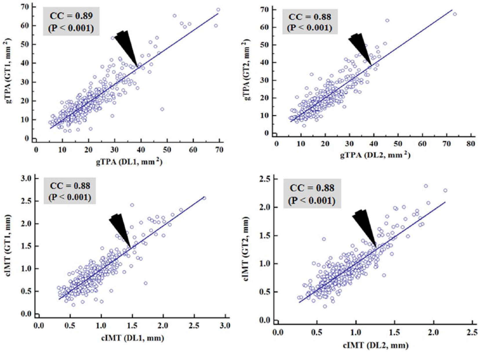
CC plots of gTPA (DL) versus gTPA (GT) and cIMT (DL) versus cIMT (GT) (a) gTPA (DL1) versus gTPA (GT1) (b) gTPA (DL2) versus gTPA (GT2) (c) cIMT (DL1) versus cIMT (GT1) (d) cIMT (DL2) versus cIMT (GT2).

From the above discussions, we conclude that risk factors like LDL, BMI, age, hypertension, and diabetes played a prominent role in cutoff design of TPA and this could be a diagnostic tool for risk stratification and possibly prediction of cardiovascular events (see Kotsis et al⁵⁰).

Strengths/Weakness/Extensions

The system offers the following key advantages: (1) simplicity in gTPA computation given the cIMT and LD computation; (2) simple model for CCA subclinical atherosclerosis modeling; (3) current cIMT and LD computation models can be easily replaced by other models; (4) current model of cIMT/LD is estimated using intelligence-based strategy; and (5) the system can be extended for internal carotid artery.

In spite of several advantages, the system encounters the following limitations: (1) the model will not be suitable for multifocal and nonsubclinical subjects or subjects having plaque burden with larger plaque above the baseline; (2) only valid for cylindrical shapes such as CCA; (3) the system requires larger database validation; and (4) our model considered a simple linear solution to computing the 10-year risk for computing image-based phenotypes such as cIMT and TPA, rather than fusing CCVR factors for its nonlinearity. In spite of above challenges, the results are encouraging adapting the new technique for gTPA computation, which is equally powerful as cIMT.

Conclusions

Carotid intima-media thickness is currently well-adapted biomarker for monitoring stroke and coronary artery disease. Recently, manually computed TPA was proposed to be useful biomarker for stroke and cardiovascular risk. The manual cIMT and TPA computations are prone to interobserver and intraobserver variabilities and tedious in computations. This study presented a DL-based technique for carotid wall interface detection followed by automated cIMT, LD, and TPA measurements. Standardized 2 DL methods were used for wall detection which followed the plaque morphology. The cIMT measurement used automated standardized polyline distance method while geometric TPA (gTPA) was measured using the concept of cylinder fitting for CCA and only requires cIMT and lumen diameter (LD). The CC between gTPA and cIMT using DL and manual proves gTPA as an equally powerful carotid risk biomarker like cIMT. Given the cIMT and LD, cylindrical fitting was observed as a fast method for gTPA measurements.

Footnotes

Appendix A

Appendix B

Appendix C

Appendix D

Appendix E

List of Abbreviations/Symbols.

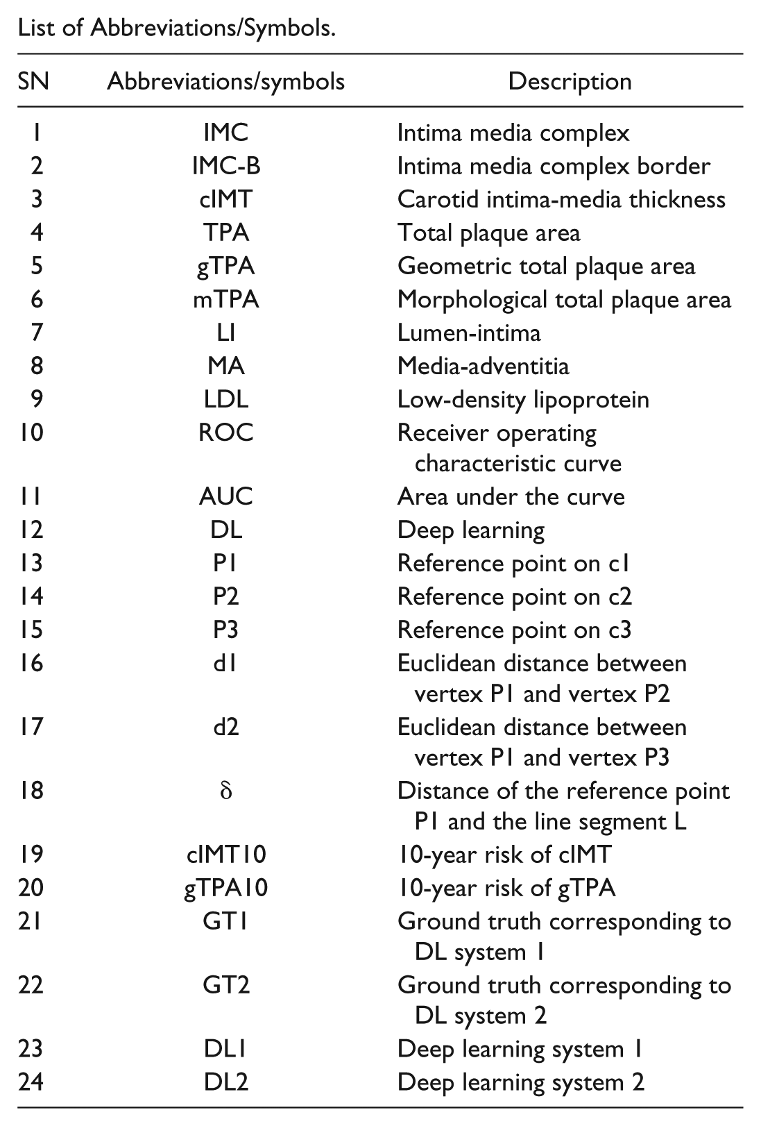
SN	Abbreviations/symbols	Description
1	IMC	Intima media complex
2	IMC-B	Intima media complex border
3	cIMT	Carotid intima-media thickness
4	TPA	Total plaque area
5	gTPA	Geometric total plaque area
6	mTPA	Morphological total plaque area
7	LI	Lumen-intima
8	MA	Media-adventitia
9	LDL	Low-density lipoprotein
10	ROC	Receiver operating characteristic curve
11	AUC	Area under the curve
12	DL	Deep learning
13	P1	Reference point on c1
14	P2	Reference point on c2
15	P3	Reference point on c3
16	d1	Euclidean distance between vertex P1 and vertex P2
17	d2	Euclidean distance between vertex P1 and vertex P3
18	δ	Distance of the reference point P1 and the line segment L
19	cIMT10	10-year risk of cIMT
20	gTPA10	10-year risk of gTPA
21	GT1	Ground truth corresponding to DL system 1
22	GT2	Ground truth corresponding to DL system 2
23	DL1	Deep learning system 1
24	DL2	Deep learning system 2

Declaration of Conflicting Interests

The author(s) declared no potential conflicts of interest with respect to the research, authorship, and/or publication of this article.

Funding

The author(s) received no financial support for the research, authorship, and/or publication of this article.

References

Benjamin

Blaha

Chiuve

SE.

Heart disease and stroke statistics—2017 update: a report from the American Heart Association. Circulation. 2017;135(10): e146-e603.

Cardiovascular Disease. Date unknown. http://www.who.int/cardiovascular_diseases/en/. Accessed September 28, 2018.

O’leary

Daniel H.

Polak

Joseph F.

Kronmal

Richard A.

Manolio

Teri A.

Burke

Gregory L.

Wolfson

Sidney K.

Jr.

Carotid-artery intima and media thickness as a risk factor for myocardial infarction and stroke in older adults. N Engl J Med. 1999;340(1):14-22.

Libby

Geng

Sukhova

Simon

Lee

RT.

Molecular determinants of atherosclerotic plaque vulnerability. Ann N Y Acad Sci. 1997;811:134-142; discussion 142-145.

Saba

Banchhor

Londhe

, et al. Web-based accurate measurements of carotid lumen diameter and stenosis severity: an ultrasound-based clinical tool for stroke risk assessment during multicenter clinical trials. Comput Biol Med. 2017;91:306-317.

Molinari

Meiburger

Zeng

, et al. “Automated carotid IMT measurement and its validation in low contrast ultrasound database of 885 patient indian population epidemiological study: results of AtheroEdge® software” Int Angiol. 2012;31(1):42-53.

Patel

Suri

Singh

, et al. A review on atherosclerotic biology, wall stiffness, physics of elasticity, and Its ultrasound-based measurement. Curr Atheroscler Rep. 2016;18(12):83.

Saba

Jain

Suri

, et al. Plaque tissue morphology-based stroke risk stratification using carotid ultrasound: a polling-based PCA learning paradigm. J Med Syst. 2017;41(6):98.

Laine

Sanches

Suri

JS.

Ultrasound imaging: advances and applications. New York, NY: Springer-Verlag; 2012.

10.

Saba

Sanches

Pedro

, et al. eds. (2014). Multi-modality atherosclerosis imaging and diagnosis. New York: Springer.

11.

Suri

Kathuria

Molinari

, eds. Atherosclerosis Disease Management. 1st ed. New York, NY: Springer-Verlag; 2011.

12.

Bots

ML.

Carotid intima-media thickness as a surrogate marker for cardiovascular disease in intervention studies. Curr Med Res Opin. 2006;22(11):2181-2190.

13.

Nambi

Chambless

Folsom

AR.

Carotid intima-media thickness and presence or absence of plaque improves prediction of coronary heart disease risk: the ARIC (Atherosclerosis Risk in Communities) study. J Am Coll Cardiol. 2010;55(15):1600-1607.

14.

Spence

Eliasziw

DiCicco

Hackam

Galil

Lohmann

Carotid plaque area: a tool for targeting and evaluating vascular preventive therapy. Stroke. 2002;33(12):2916-2922.

15.

Spence

Hegele

RA.

Noninvasive phenotypes of atherosclerosis: similar windows but different views. Stroke. 2004;35(3):649-653.

16.

Alsulaimani

Gardener

Elkind

MSV

Cheung

Sacco

Rundek

Elevated homocysteine and carotid plaque area and densitometry in the northern Manhattan study. Stroke. 2013;44(2):457-461.

17.

Mathiesen

Johnsen

Wilsgaard

Bønaa

Løchen

Njølstad

Carotid plaque area and intima-media thickness in prediction of first-ever ischemic stroke: a 10-year follow-up of 6584 men and women: the Tromsø study. Stroke. 2011;42(4):972-978.

18.

Herder

Johnsen

Arntzen

Mathiesen

EB.

Risk factors for progression of carotid intima-media thickness and total plaque area: a 13-year follow-up study: the Tromsø study. Stroke. 2012;43(7):1818-1823.

19.

Kamycheva

Johnsen

Wilsgaard

, et al. Evaluation of serum 25-hydroxyvitamin D as a predictor of carotid intima-media thickness and carotid total plaque area in nonsmokers: the Tromsø Study. Int J Endocrinol. 2013;2013:305141. doi: 10.1155/2013/305141.

20.

Romanens

Mortensen

Sudano

Szucs

Adams

Extensive carotid atherosclerosis and the diagnostic accuracy of coronary risk calculators. Prev Med Rep. 2017;6:182-186.

21.

Adams

Bojara

Schunk

Early diagnosis and treatment of coronary heart disease in asymptomatic subjects with advanced vascular atherosclerosis of the carotid artery (type III and IV b findings using ultrasound) and risk factors. Cardiol Res. 2018;9(1):22-27.

22.

Molinari

Zeng

Suri

JS.

Intima-media thickness: setting a standard for a completely automated method of ultrasound measurement. IEEE Trans. IEEE Trans Ultrason Ferroelectr Freq Control. 2010;57(5):1112-1124.

23.

Molinari

Pattichis

Zeng

, et al. Completely automated multiresolution edge snapper—a new technique for an accurate carotid ultrasound IMT measurement: clinical validation and benchmarking on a multi-institutional database. IEEE Trans Image Process. 2012;21(3):1211-1222.

24.

Linhart

Gariepy

Giral

Levenson

Simon

Carotid artery and left ventricular structural relationship in asymptomatic men at risk for cardiovascular disease. Atherosclerosis. 1996;127(1):103-112.

25.

Ikeda

Dey

Sharma

, et al. Automated segmental-IMT measurement in thin/thick plaque with bulb presence in carotid ultrasound from multiple scanners: stroke risk assessment. Comput Methods Programs Biomed. 2017;141:73-81.

26.

Ikeda

Araki

Dey

, et al. Automated and accurate carotid bulb detection, its verification and validation in low quality frozen frames and motion video. Int Angiol. 2014;33(6):573-589.

27.

Biswas

Venkatanareshbabu

Luca

, et al. Deep learning fully convolution network for lumen characterization in diabetic patients using carotid ultrasound: a tool for stroke risk. Med Biol Eng Comput 2018: 1-22.

28.

Molinari

Zeng

Suri

JS.

An integrated approach to computer- based automated tracing and its validation for 200 common carotid. J Ultrasound Med. 2010;29:399-418.

29.

Molinari

Rajendra Acharya

Zeng

Meiburger

Suri

. Completely automated robust edge snapper for carotid ultrasound IMT measurement on a multi-institutional database of 300 images. Med. Med Biol Eng Comput. 2011;49(8):935-945.

30.

Molinari

Meiburger

Nicolaides

Suri

JS.

CAUDLES-EF: carotid automated ultrasound double line extraction system using edge flow. J Digit Imaging. 2011;24:129-162.

31.

Saba

Molinari

Meiburger

Acharya

Nicolaides

Suri

JS.

Inter- and intra-observer variability analysis of completely automated cIMT measurement software (AtheroEdge^TM) and its benchmarking against commercial ultrasound scanner and expert Readers. Comput Biol Med. 2013;43(9):1261-1272.

32.

Ikeda

Gupta

Dey

, et al. Improved correlation between carotid and coronary atherosclerosis SYNTAX score using automated ultrasound carotid bulb plaque IMT measurement. Ultrasound Med Biol. 2015;41(5):1247-1262.

33.

Saba

Banchhor

Suri

, et al. Accurate cloud-based smart IMT measurement, its validation and stroke risk stratification in carotid ultrasound: a web-based point-of-care tool for multicenter clinical trial. Comput Biol Med. 2016;75:217-234.

34.

Acharya

Rajendra

MRK

Mookiah

, et al. Evolutionary algorithm-based classifier parameter tuning for automatic ovarian cancer tissue characterization and classification. Ultraschall in der Medizin-European J Ultrasound. 2014;35(3): 237-245.

35.

Acharya

Sree

Kulshreshtha

, et al. GyneScan: an improved online paradigm for screening of ovarian cancer via tissue characterization. Technol Cancer Res Treat. 2014; 13(6):529-539.

36.

Pareek

Acharya

Sree

, et al. Prostate tissue characterization/classification in 144 patient population using wavelet and higher order spectra features from transrectal ultrasound images. Technol Cancer Res Treat. 2013;12(6):545-557.

37.

Shrivastava

Londhe

Sonawane

Suri

JS.

Reliable and accurate psoriasis disease classification in dermatology images using comprehensive feature space in machine learning paradigm. Expert Syst Appl. 2015;42(15-16):6184-6195.

38.

Maniruzzaman

Rahman

Al-MehediHasan

, et al. Accurate diabetes risk stratification using machine learning: role of missing value and outliers. J Med Syst. 2018;42(5):1-17.

39.

Kumar

Araki

Rajan

, et al. Accurate lumen diameter measurement in curved vessels in carotid ultrasound: an iterative scale-space and spatial transformation approach. Med Biol Eng Comput. 2017;55(8):1415-1434.

40.

Kuppili

Biswas

Sreekumar

, et al. Extreme learning machine framework for risk stratification of fatty liver disease using ultrasound tissue characterization. J Med Syst. 2017;41(10):152.

41.

LeCun

Bengio

Hinton

Deep learning. Nature. 2015;521(7553):436-44.

42.

Klein

Hegele

Hackam

Koschinsky

Huff

Spence

JD.

Lipoprotein(a) is associated differentially with carotid stenosis, occlusion, and total plaque area. Arterioscler Thromb Vasc Biol. 2008;28(10):1851-1856.

43.

Perez

Garcia

Spence

Armando

LJ.

Adding carotid total plaque area to the Framingham risk score improves cardiovascular risk classification. Arch Med Sci. 2016;12(3):513-520.

44.

Molinari

Liboni

Giustetto

Badalamenti

Suri

JS.

Automatic computer-based tracings (ACT) in longitudinal 2-D ultrasound images using different scanners. J Mech Med Biol. 2009;9(4):481-505.

45.

Meiburger

Molinari

Acharya

, et al. Automated carotid artery intima layer regional segmentation. Phys Med Biol. 2011;56(13):4073-4090.

46.

Biswas

Kuppili

Araki

, et al. Deep learning strategy for accurate carotid intima-media thickness measurement: an ultrasound study on Japanese diabetic cohort. Comput Biol Med. 2018;98:100-117.

47.

Long

Shelhamer

Darrell

(2015) Fully convolutional networks for semantic segmentation. In Proceedings of the IEEE conference on computer vision and pattern recognition (pp. 3431-3440).

48.

Spence

Solo

Resistant atherosclerosis: the need for monitoring of plaque burden. Stroke. 2017;48(6):1624-1629.

49.

Dong

Della-Morte

Cabral

, et al. Sirtuin/uncoupling protein gene variants and carotid plaque area and morphology. Int J Stroke. 2015;10(8):1247-1252.

50.

Kotsis

Jamthikar

Araki

, et al. Echolucency-based phenotype in carotid atherosclerosis disease for risk stratification of diabetes patients. Diabetes Res Clin Pract. 2018;143:322-331.