Fuel-saving ship route using the Navy’s ensemble meteorological and oceanic forecasts

Abstract

Fuel conservation and carbon reduction are important issues in current naval operations. Optimal ship route (i.e. minimum fuel consumption) depends on specific ship platform characteristics and near real-time environment such as weather, ocean waves, and ocean currents. The environmental impact of shipping can be measured on different spatial and temporal scales. As a vital component of the smart voyage planning (SVP) decision aid, the US Navy’s meteorological and oceanographic (METOC) forecast systems play an important role in optimal ship routing, which enables fuel savings in addition to the aid of heavy weather avoidance. This study assesses the impact of METOC ensemble forecast systems on optimal ship route. Tests of the SVP decision aid tool are also conducted for operational fleet use and concept of operations for the USS Princeton guided missile cruiser (CG)-59 in a sea trial test following the 2012 Rim of the Pacific exercises.

Keywords

Navy operational global atmospheric prediction system WaveWatch III Navy coastal ocean model brier score ensemble prediction fuel conservation and carbon reduction fuel consumption fuel-saving ship routing smart voyage planning (SVP) decision aid ensemble SVP modeling ship tracking and routing system

1. Introduction

Ship routing involves optimal control from the meteorological and oceanographic (METOC) effects on the navigation to specific ship platform characteristics. For instance, the course of a ship between two given points may be determined by minimal fuel consumption with course and speed of the ship as control variables. To compute an optimal path, all the ship characteristics such as platform hull form, power curve, and loading, as well as all the disturbing forces that could influence the ship on its way, such as winds, waves, and currents (environmental disturbing forces),¹ must be known.

By applying the available surface and upper air forecasts to transoceanic shipping, it is possible to effectively avoid heavy weather while generally sailing shorter routes than previously. The development of computers, the internet and communications technology has made weather routing available to nearly everyone afloat. Criteria for route selection reflect a balance between the captain’s desired levels of speed, safety, comfort, and consideration of operations such as fleet maneuvers, fishing, towing, etc. Ship weather routing services are being offered by many nations. Also, several private firms provide routing services to shipping industry clients. Additionally, several PC-based software applications have become available, making weather routing available to virtually everyone at sea.

The smart voyage planning (SVP) decision aid tool has been identified as a key technology for the US Navy, capable of assisting with the fleet energy saving goals. The US Navy’s Task Force Energy has identified SVP as a key technology, capable of reducing the Navy’s carbon footprint (i.e. amount of CO₂ emission in a year) and accomplishing energy saving goals. Commercial SVP tools currently use weather, ocean waves and specific ship platform characteristic data to develop optimal transit routes which save on the order of 5% in fuel expenditures. Today’s robust Navy METOC models and forecasts, combined with improved algorithms, enable fuel savings in addition to the aid of heavy weather avoidance. However, with enhanced model output, the improvement in the least cost route, as compared to the best possible route using actual analysis environmental data in SVP models, has not been thoroughly studied.

Questions arise: Which environmental factors carry the highest sensitivity for the SVP models? What is the improvement in the least cost route as compared to the best possible route using actual analysis environmental data in SVP models? What additional incremental efforts are required to optimize ship routing and yield drastic improvements in fuel efficiency? To answer these questions, sensitivity studies on the SVP models have been conducted in this study to analyze the dependence of fuel savings on the ship characteristics (speed, track, ship limits) and METOC environment such as winds, waves, and currents from Navy’s modeled and reanalyzed data. The route optimization with SVP is intended to minimize the fuel consumption while maintaining ship safety. A concept of operation (CONOPS) test was conducted following the 2012 Rim of the Pacific (RIMPAC) exercises with the USS Princeton CG-59. During the CONOPS test, trials were used to identify how the SVP results could be used by ship routing personnel to assist in analyzing alternatives and aiding ship routing decisions.

2. Fuel Consumption

Consider a ship moving in the ocean. Each point of the ocean is characterized by certain properties describing the severity of the sea conditions at that particular location and time. Clearly, the motion is affected by the position of the ship in the sea because the mean added resistance will be a function of space and time. This is not the case in calm water, where the problem is time and space invariant. Recognizing this, a natural choice for the ‘state’ of the system is the ship’s location on the sea surface. This location should be referenced to an appropriate coordinate system. By definition, a state should have the property of describing the current condition and prior history of a process in sufficient detail to allow evaluation of current alternatives.

Let (x, y) be the coordinates representing east and north directions. The state vector is the position vector x(t) = [x(t), y(t)]^T with the superscript ‘T’ denoting transpose. The ship position is predicted by

\begin{matrix} \frac{dx}{dt} = U (t) \cos p (t) + C_{1} (t, x, y), \\ \frac{dy}{dt} = U (t) \sin p (t) + C_{2} (t, x, y), \end{matrix}

(1)

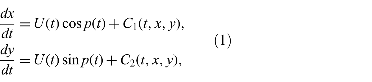
where (C₁, C₂) are the components of the ocean current velocity. The control is the ship speed (U) and course (p) measured from true north. The fuel rate in the engine is given by the product of the specific fuel consumption (S) and the break power (P_B):

q = S P_{B} .

(2)

The break power can be expressed as

P_{B} = \frac{R_{total}}{η_{D} η_{TRM}}

(3)

where η_D is the quasi-propulsive coefficient; η_TRM is the transmission efficiency; and R_total is the total towing resistance. The total tow resistance is decomposed by

R_{total} = R_{calm} (U) + {\bar{R}}_{w} (u, x, t) .

(4)

Thus, the fuel consumption can be calculated by

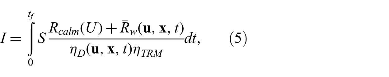
I = \int_{0}^{t_{f}} S \frac{R_{calm} (U) + {\bar{R}}_{w} (u, x, t)}{η_{D} (u, x, t) η_{TRM}} dt,

(5)

which is very sensitive to ship speed. For a naval gas turbine, it increases rapidly with ship speed, by approximately 1% to 4% per knot at moderate speeds and approximately 9% per knot at high speeds. Fuel consumption efficiency in gas turbine ships is also very sensitive to lower speeds. Optimizing the ship speed profile during transit can yield significant fuel savings. Realistic propulsion fuel curves are used for the various classes of ships. A typical gas turbine propulsion plant fuel curve is identified in Figure 1(a). A ship’s fuel consumption rate increases significantly with moderate waves, wind, and current. At constant speed, fuel consumption in sea-state 4, with 1 knot current, increases by approximately 10% over the calm water value. Therefore, optimizing the ship route together with the speed profile to reduce drag by avoiding adverse sea-state conditions during transit can yield even greater fuel savings. This effect is illustrated in Figure 1(b). Other factors affecting fuel consumption are wind, hull/propeller fouling condition, reduced propulsive efficiency, ships service loads, plant operation mode (e.g. full plant, trail shaft), and propeller pitch control system.

Figure 1.

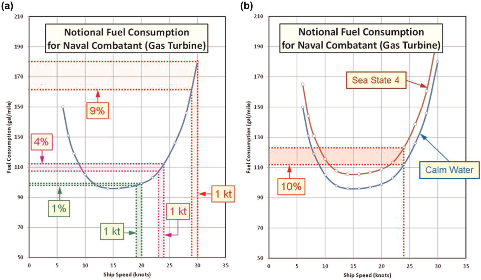
Fuel consumption curve and relationship to speed: (a) general information, and (b) sensitivity to sea state.

Speed reduction curves are often used for fuel savings. They indicate the effect of head, beam, and following seas of various significant wave heights on the ship’s speed. Each vessel will have its own speed reduction curves, which vary widely according to hull type, length, beam, shape, power, and tonnage. Figure 2 shows the speed reduction curves for the DDG-58 class ships. Due to timeliness, the commonly used methods for fuel reduction in the shipping industry such as ‘slow-steaming’ and ‘super-slow-steaming’ might not be suitable for the Navy. Mathematically, the fuel-saving ship routing is to minimize the fuel consumption (I)²

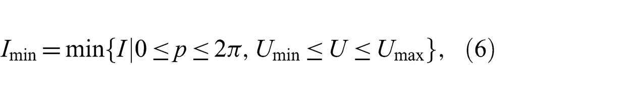
I_{min} = min {I | 0 \leq p \leq 2 π, U_{min} \leq U \leq U_{max}},

(6)

subject to the given range of the ship speed [U_min, U_max]; the dynamic constraint (1); speed reduction curves; a safety constraint; control bounds maximum allowable wave height in head, beam, and following seas; maximum allowable true and relative wind speeds; tropical cyclone avoidance limits for 18 m/s (35 knots) and 26 m/s (50 knots) wind circles; land mass avoidance; initial conditions; and final time

x (0) = [\begin{matrix} x (0) \\ y (0) \end{matrix}], t_{f} prescribed .

(7)

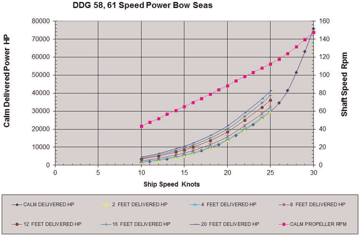
Thus, the METOC variables such as winds, significant wave height, ocean current velocity, and tropical cyclone track and radius affect the fuel consumption (I) directly through changing the ship location x [see equations (1) and (4)] and indirectly through changing the constraints in the optimization process depicted by equation (6). Accurate METOC prediction takes an important role in SVP.

Figure 2.

DDG 58 speed reduction curves for bow seas.

3. Navy METOC Models and DATA

3.1. Navy Operational Global Atmospheric Prediction System

The Navy operational global atmospheric prediction system (NOGAPS) is a high resolution global numerical weather prediction (NWP) model (see the website: http://www.nrlmry.navy.mil/nogaps_his.htm). Its development and operation is a joint activity of the Naval Research Laboratory (NRL) and the Navy’s Fleet Numerical Meteorology and Oceanography Center (FNMOC). The NOGAPS is spectral in the horizontal and energy-conserving finite difference (sigma coordinate) in the vertical. The model top pressure is set at 0.04 hPa; however, the first velocity and temperature level is approximately 0.07 hPa. The variables used in dynamic formulations are vorticity and divergence, virtual potential temperature, specific humidity, surface pressure, skin temperature, and ground wetness. NOGAPS is also a primary tropical cyclone forecast tool for forecasters at the Joint Typhoon Warning Center. NOGAPS uses a four-dimensional variational analysis scheme for data assimilation. Besides using conventional observations (surface, rawinsonde, pibal, and aircraft), the analysis employs both direct radiance (brightness temperature) and derived soundings from NOAA and Defense Meteorological Satellite Program polar-orbiting satellite instruments. The instruments utilized include the advanced microwave sounding unit-A, atmospheric infrared sounder, infrared atmospheric sounding interferometer, special sensor microwave imager/sounder (SSMI/S), and microwave humidity sounder. Additional soundings are derived via GPS-radio occultation measurements. Surface marine wind speeds are assimilated using several different scatterometers (ASCAT, ERS-2, WindSat, SSMI) while winds aloft are estimated from atmospheric motion vector measurements. These measurements consist of water vapor, infrared, and visible satellite imagery, such as geostationary, moderate resolution imaging spectroradiometer, advanced very high resolution radiometer, and low Earth orbit (. NOGAPS provides forcing fields for mesoscale weather prediction; tropical cyclone prediction; aerosol prediction; ocean, wave, and ice prediction; and aircraft and ship routing applications. NOGAPS also forms the backbone of the Navy’s ensemble prediction system, which provides global forecasts up to 10 days. NOGAPS was replaced by the Navy General Environmental Model (NAVGEM) in March 2013.

3.2. WaveWatch III

WaveWatch III (WW3) is a third generation wave model developed at the NOAA National Centers for Environmental Prediction.³ It uses the statistical properties of waves to predict the sea state at a point, rather than trying to predict individual waves. The full sea state at any point over the ocean consists of the overlaying (or more technically, the superposition) of waves with different characteristics (wavelength and amplitude) arriving from all directions. Both the global and regional WW3 models predict the energy spectrum of these waves over a range of discrete frequencies and directions, using what is known as a wave action density equation.

3.3. Navy operational global ocean model

The US Navy Coastal Ocean Model (NCOM) is a three-dimensional ocean circulation model developed by the Naval Research Laboratory (NRL) and operated by the Naval Oceanographic Office.^4,5 It is used as the basis for the forecast of global ocean temperature, salinity, and current velocity. NCOM is a free-surface, primitive-equation model based primarily on two other models: the Princeton ocean model and the sigma/z-level model.⁶ In its global configuration, NCOM implements a curvilinear horizontal grid designed to maintain a grid-cell horizontal aspect ratio near 1.⁷ Horizontal resolution varies from 19.5 km near the equator to 8 km or finer in the Arctic, with mid-latitude resolution of about 1/8° latitude (~14 km). Horizontal resolution has been sacrificed to allow increased vertical resolution. To improve the detail of upper-ocean dynamics, a maximum 1-m upper level thickness in a hybrid sigma/z vertical configuration with 19 terrain-following sigma-levels in the upper 137 m over 21 fixed-thickness z-levels extending to a maximum depth of 5500 m is used. Model depth and coastline are based on a global 2-minute bathymetry produced at the NRL. The 1/8^o global NCOM was also replaced by a 1/12° global hybrid coordinate ocean model (HYCOM) in March 2013. Data assimilation is via 3DVAR. NCOM is still used for regional (1/30°) domains.

3.4. Data

Four-time daily data of winds, waves, and ocean currents were obtained from FNMOC and used as the environmental input into the SVP model. The data of tropical cyclone tracks and radius for the SVP model were extracted from the Joint Typhoon Warning Center. The surface winds were the output of the NOGAPS model. The ocean waves/swells (sea states) were the output of WW3 model with the NOGAPS winds as the forcing function (input). The ocean currents were the output of global NCOM, which used atmospheric forcing function from the NOGAPS, with latent and sensible heat fluxes calculated internally using the NCOM sea surface temperature. The present daily NCOM model consisted of a 72-hour hindcast to assimilate fields, including recent observations and a 72-hour forecast. Data assimilation is based on global profiles of temperature and salinity derived using operational sea-surface fields and in situ data within the modular ocean data assimilation system (MODAS).^8,9 The climatology of surface winds, waves/swells, and currents was also generated at FNMOC for the last 15 years. The bathymetry data was extracted from the Navy’s Digital Bathymetric Data Base Variable Resolution with 2-minute horizontal resolution. A 12 m depth is used as the cutoff for navigable waters, i.e. depth less than 12 m is referred to as shallow water, and depth deeper than 12 m is referred to deep water.

3.5. Ensemble modeling

Ensemble METOC numerical forecast models are excellent tools for quantifying the uncertainties in natural environments that impact tactical operations. The key concept is that ensemble modeling takes us from a deterministic (one answer, no indication of uncertainty) to a probabilistic (one answer with a plus or minus level of skill) forecast. The latter allows sailors to assess the risk associated with the recommended courses of action. Usually, ensembles account for three sources of uncertainty in weather forecast models. The first is errors introduced by uncertain initial conditions. The second is errors introduced by uncertain boundary conditions.¹⁰ The third is errors introduced because of imperfections in the model, such as the discretization and initial uncertainty. The verified weather pattern should be consistent with ensemble spreads and the amount of spread should be related to the confidence of certain weather events occurring. Therefore, ensembles can be a key in increasing forecast skill for better route predictions.

Model forecasts can be sensitive to the design of the model as well as to the initial conditions. Each model configuration approximates the actual behavior of the atmosphere differently, so this introduces another source of forecast uncertainty. It is not possible to construct an NWP model that includes the behavior of the atmosphere in every detail at infinitely high resolution. The FNMOC global ensemble forecast system (GEFS) has 80 NOGAPS perturbed members at T159L42 resolution run for 6-hour forecasts (used to produce the perturbations for the next cycle), where 20 of these members continue the forecast out to 16 days. Output from the model runs are on one-degree by one-degree spherical grids. For production of probabilities and other statistics, the members also include one-degree grids from the deterministic NOGAPS 42-level T319 forecast and the T319L42 forecast lagged by 12 hours, for a total of 32 members. FNMOC also runs 32 members of the wave model ensemble forced by winds from the NOGAPS ensemble forecast system. The wave model runs on a 1°×1° resolution global grid on a 12 hour update cycle. The WW3 EFS members forecast out to 10 days (240 hours). Unlike the NOGAPS EFS, the ‘first guess’ wave field is not perturbed; rather the variability among the members comes from the variability of the wind forcing.

4. SVP

SVP is an advanced computerized optimization of ship operations offering intelligent speed and route management that can significantly reduce fuel consumption and associated emissions while maintaining the same overall transit time.^11–13 A ship’s speed and route can be optimized based on the wind, waves, and currents, taking into account the ship’s performance criteria such as hull shape, horsepower, load, trim, ballast, pitch and roll limits, and other factors (Figure 3). This SVP program incorporates advanced voyage optimization algorithms that include the ship’s hull design, propulsion systems, and sea keeping models, as well as user-defined safe operating limits.

Figure 3.

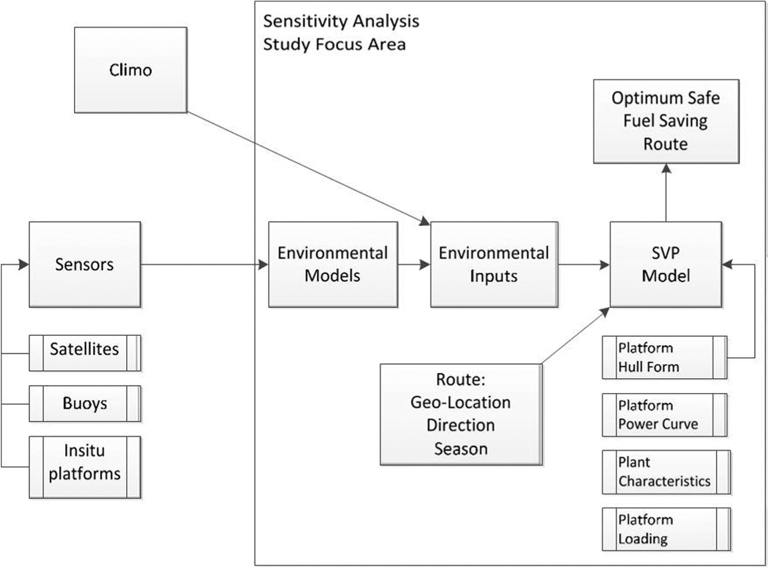
Flow chart of SVP with METOC model input.

Once specific environmental model outputs are identified, follow-on efforts can be made to improve METOC forecast skills and model outputs to enhance near term and medium term forecast accuracy/precision. Methods such as ensembles and improved air/ocean coupled numerical models and/or increased resolution may be utilized. Use of assimilated forcing data from various sensors and climatology may also enhance model output and reduce variance. Utilizing targeted improved forecast weather, wave, and current accuracy, SVP models will ensure a least cost track, thereby maximizing fuel savings while sailing safe routes. Sensitivity analysis methods can utilize the best outcomes for SVP model input (Figure 3). Specifically, weather, wave and ocean current model outputs will be used as inputs into the SVP model. To enable the sensitivity studies, the following data fields were input into the model using 2010–2011 archived environmental data and realistic empirical data for vessel platform characteristics: waves (period/swell/height), winds, currents, platform hull forms, ship power curves and plant L/U (ship length versus ship speed), and ship loading characteristics.

5. Ship route engine design

5.1. Ship tracking and routing system

The ship tracking and routing system (STARS) is a ship route optimization suite of software provided for research by FNMOC and modified for use in NRL-Monterey computing environment.¹⁴ The model outputs an optimum route which is defined as the route that completes the voyage within time limits and with the least amount of fuel expended, while keeping the vessel from exceeding the wind and sea limits specified by competent authority. STARS utilizes a Dijkstra exhaustive search algorithm for minimum cost using the follows steps: (1) creating a 3-D point grid (latitude, longitude, time to point) based on user-specified departure/arrival locations and times and min/max ship speed; (2) grid aligning with the great circle (GC) route and internally defined grid spacing or utilizes manually inputted upper and lower boundary points; (3) exhaustively searching all feasible routes (i.e. all possible forward-traversing connections between grid nodes that meet the constraints); and (4) examining both the minimum and maximum ship speeds from all points at the previous stage for each geographic grid location. Note that manually inputted upper and lower boundary points were used for this research with the bounded grid resolution of 300×60,¹⁴

METOC inputs of winds and seas provide information to the algorithm that calculates the fuel expended over a number of test routes and selects the optimized route (courses and speeds) to sail that will use the least fuel and avoid weather limits that the user specifies. The input parameters are: swell direction, swell height, swell period, surface (10 m height) wind speed and direction, wind wave direction, wind wave height, and wind wave period. The wind and sea limits used were 18 m/s (35 knots) and 3.66 m (12 foot), in accordance with US Navy standing operational order requirements.

The ships are sometimes pushed forward (driving force) and sometimes pulled backward (resisting force) by the winds, seas, and currents. It is advantageous to use (avoid) the driving (resisting) force for any ship. The fuel expended over the route is directly related to the relative winds and seas that resist the forward advance of the ship and the distance/time that the engine runs. The application of favorable winds, seas, and currents can reduce fuel consumption. For the favorable (unfavorable) case, the greater the amplitude of the relative winds, seas, and currents, the greater the driving (resisting) force, and the longer (higher) the engine runs, and the less (more) the fuel that is expended. Thus, calculations of relative winds, seas, and currents are important in the ship routing (course and speed).¹⁴

5.2. SVP decision aid

The SVP Decision Aid (SVPDA, Figure 4(a)) uses a cost evaluation function,¹¹

C (Ω, N + 1) = \sum_{i = 1}^{N} α_{i} (Ω, U, M) + β (Ω_{N + 1})

(8)

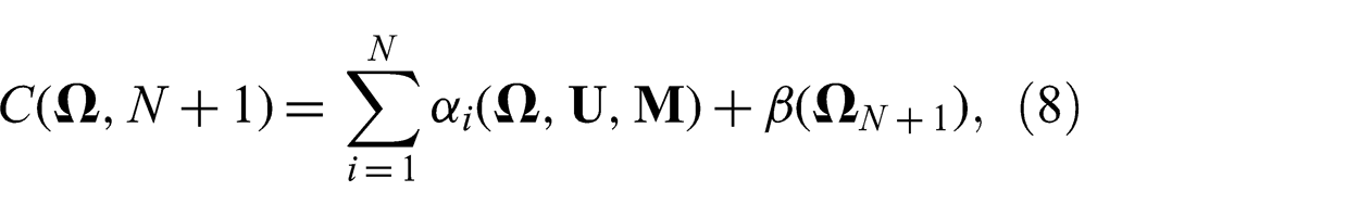
to minimize the fuel consumption for stage (N+ 1) with the operating cost α_i at stage i (= 1, 2, …, N) and the terminal coast β, subject to the constraints within the predicted grid system, allowable transitions between grids, and allowable motion. Here, α_i is a function of Ω, U, M and β is a function of Ω_N+1. Ω is the state variable containing the navigational coordinates and time. U is the control variable consisting of a set of allowable forward-transitions between present and next states as well as a set of discretized power output. M is the generalized ship motion and sea-keeping index, and the subscript “i” is the stage variable (monotonically increasing integer) related to the headway and consistent with the set of allowable forward transitions at each stage. Usually, α_i and β are nonlinear functions. The ship route engine has the overall objective of minimizing fuel consumption within environmental and geographic constraints. The optimizer calls the cost evaluation function many times, so it must be computationally efficient. The cost evaluation function (C) depends on ship’s hull friction, power plant fuel use, ocean wave height/period/velocity swell height/period/velocity (from WW3), ocean current velocity (from NCOM), and surface winds (from NOGAPS).

Figure 4.

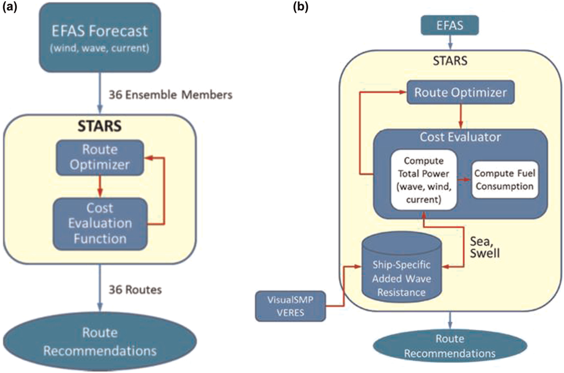
Flow chart for (a) basic routing engine, and (b) routing engine with improved cost prediction.

Long running calculations (e.g. added wave resistance) are cached in a data-store and interpolated at the routing engine run-time. Short running cost calculations are performed in line. Estimated added resistance in waves is done using first order principle computational tools such as the ship motions program and vessel responses. All above costs are then combined to determine a total fuel consumption rate in the cost evaluator as identified in Figure 4b.

5.3. Routine options

Three primary options are available in running the SVP software: WEAX, SPEEDX, and ROUTEX. WEAX uses given waypoints, returns a route with intermediate synoptic reporting points interspersed, and reports weather and any warnings along the route. This option is useful for determining the actual cost of a route when run in an analysis forecast environment. SPEEDX uses given waypoints, adjusts speeds between points to avoid bad weather, and is useful for divert routing. ROUTEX uses given start and end points or boundary limits, constructs grids within those limits, and determines the optimum route within the grid based on fuel efficiency and weather/bathymetry limits.

An overview of the current route optimization algorithm is outlined as follows. It constructs a grid between the start and end points of the track. If the user has specified upper and lower boundary lines, these are used. The grid not only has two-dimensional latitude/longitude locations, but also a third dimension of time stages. That is, the ship can arrive at each location at a variable time. Using the maximum and minimum speeds for the ship specified by the user, the maximum and minimum times to each of the grid points from all of the previous grid points are calculated. Similar calculations are done for maximum time and minimum speed.

The optimization loop (nested) function (or feature) is depicted as follows. For each point in the X-direction (along the track), Y-direction (across the track) and each time increment (1 hour), compute time to travel from each previous y-state (point in last Y column) to the current point looping over all possible arrival times from the previous state from minimum to maximum arrival time at the point. If there is a solution at the previous y-state; if the speed required is greater than the minimum speed, and less than the maximum speed; if no land is encountered for the track; and if no environmental limits are exceeded for the track, compute the total power (HP-hours or fuel) to get to the current point. If the total power is less than the total power to get to this point at this time from any of the previous y-state points, save it as the best solution for this y-state. Loop through all the time solutions for the entire route, find the solution with an arrival time that does not exceed the estimated time of arrival which has the least power cost. If no valid route is found, return an error message and stop processing. If a valid route is found, the track is traversed backward through the links to save the best path in common for subsequent processing.

6. Ensemble SVP modeling

6.1. Ensemble members

The initial conditions for the FNMOC GEFS were produced by the four-dimensional NRL atmospheric variational data assimilation system-accelerated representer (NAVDAS-AR). The 42 level T319 spectral truncation analysis produced by this system was used for the T319L42 control (deterministic) forecast, and also truncated to T159 and perturbed using the Ensemble Transform (ET) technique for the GEFS. For statistical analysis, the members also included one-degree grids from the deterministic NOGAPS 42-level T319 forecast and the T319L42 forecast lagged by 12 hours, for a total of 32 members. FNMOC also ran a 32 member wave model (WW3) ensemble forced by winds from the NOGAPS Ensemble Forecast System on a 1°×1° global grid on a 12 hour update cycle. The WW3 EFS members forecasted up to 10 days (240 hours). Unlike the NOGAPS EFS, the ‘first guess’ wave field was not perturbed; rather the variability among the members comes from the variability of the wind forcing.

6.2. Modeling strategy

The METOC ensemble that is downloaded from a central site or from multiple sites and averaged in the ensemble forecast application system (EFAS) database is referred to as the raw ensemble. The average of the raw ensemble members is called the ensemble average. The ensemble data calibration process is initiated by applying a bias-correction to every grid point and level at every forecast step (τ) that a result is needed. For the SVPDA model ensemble input, bias-correction was applied to the needed forecast parameters at 6 hour intervals across the full set of available forecasts out to TAU 240 h. For each forecast τ (6 h, 12 h, 18 h… 240 h) and at every grid point each of the ensemble members, the forecast parameter value was subtracted from the verifying analysis value. The average difference across the ensemble members between the forecast and analysis at each grid point and τ comprise the bias value at that grid point. For each forecast cycle (00Z forecast cycle and 12Z forecast cycle) a running mean of the last 30 days of 00Z and 12Z forecast bias values was then computed at each τ and grid point. Then the new 30-day running mean grid point bias-correction was applied to each ensemble member (the time span for the running mean is configurable). This data set is referred to as the bias-corrected ensemble. This process was repeated at every 12 hour forecast cycle after the raw ensemble is produced.

6.3. Brier score

The Brier Score

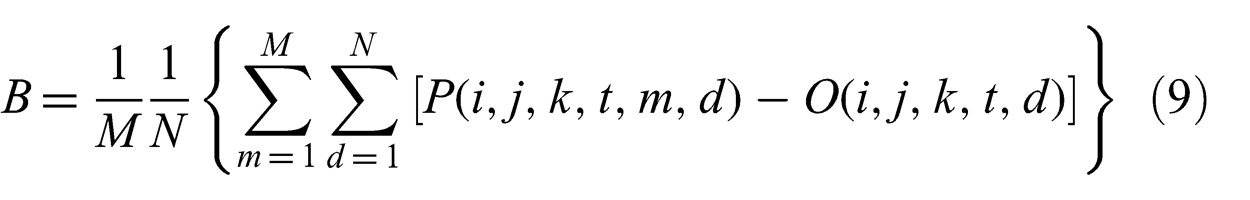
B = \frac{1}{M} \frac{1}{N} {\sum_{m = 1}^{M} \sum_{d = 1}^{N} [P (i, j, k, t, m, d) - O (i, j, k, t, d)]}

(9)

is commonly used to identify the bias of ensemble forecast. Here P is the forecast probability, O is the actual outcome of the event at instance; N is the number of model runs; M is the number of ensemble members; and d is the prediction period with d = 0 for the nowcast (near realistic).

If a wind direction forecast is needed we extract the information from the raw ensemble average. When these individual consensus forecasts are combined it is referred to as the hybrid forecast or the hybrid ensemble. This hybrid combination of forecast values can then be interfaced to the SVPDA in the same manner as provided by a deterministic forecast. When using hybrid consensus forecasts whose method varies by parameter and forecast τ, it is important to remember that the resulting forecasts are not physically/meteorologically consistent because it is a statistical result. The EFAS is interfaced to STARS (Figure 5) to derive a 35 member (16 raw ensemble members, 16 bias-corrected members, 1 raw ensemble average, 1 bias-corrected average, and 1 hybrid) ensemble of ship routes optimized for minimum fuel burn and to avoid high winds and sea-states.

Figure 5.

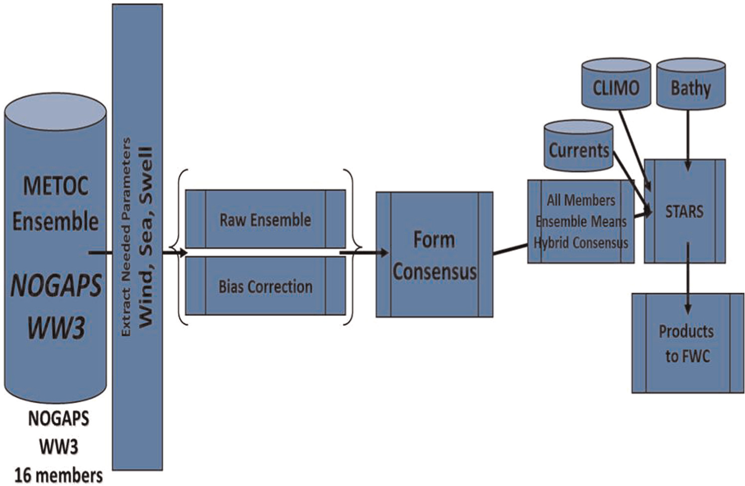
Environmental and ensemble STARS modeling.

7. Impact of METOC model forecasts

The impact of METOC model prediction on optimum ship routing can be identified by the case study. Additionally, ensemble methods were utilized for quantifying the environmental model uncertainties and improving forecast skill. The benefits of using realistic platform characteristics of various classes of naval vessels are also determined. Impacts of individual model (NOGAPS, WW3, NCOM) quality on the SVPDA route outputs are also identified. In order to try and capture variability due to space and time, the sensitivity analysis was conducted over the course of various seasons and various regional locations of the globe. The model outputs were in pure extensible markup language (XML) and required a robust scripting tool in order to parse all route output for each model run. A complex PYTHON script was written to parse the XML output file and creates a flat file in addition to several statistical figures.

7.1. Ship parameters

Three United States Naval Ships (TAO-187, DDG-90, and DDG-93) are used to identify the impact of METOC ensemble prediction on fuel-saving using the SVPDA with various METOC ensemble forecasts. Among them, TAO-187 is a fleet replenishment oiler, and DDG-90 and DDG-93 are guided missile destroyers. The ship wind speed limits are 35 knots (18 m/s) for bow, beam, and stern. The ship sea heights limits are 12 feet (3.66 m) for bow, beam, and stern. Allowable speed is between 25 knots (12.86 m/s) and 10 knots (5.14 m/s). The great circle baseline speed is 17.5 kts for TAO-187 and 16.6 kts for DDG. The number of start and ending waypoints is 2. The number of upper and lower bound waypoints is 4 each. The starting dates are 1 June 2010, 1 July 2010, 1 December 2010, and 1 June 2011. Two cases are presented here. Case-1 is the route between Diego Garcia and the Gulf of Oman with one way great circle distance of 1946.60 nm. Case-2 is the route between San Diego and Pearl Harbor with one way great circle distance of 2191.09 nm. Figure 6 shows the examples of ship routes with red color denoting the GC route.

Figure 6.

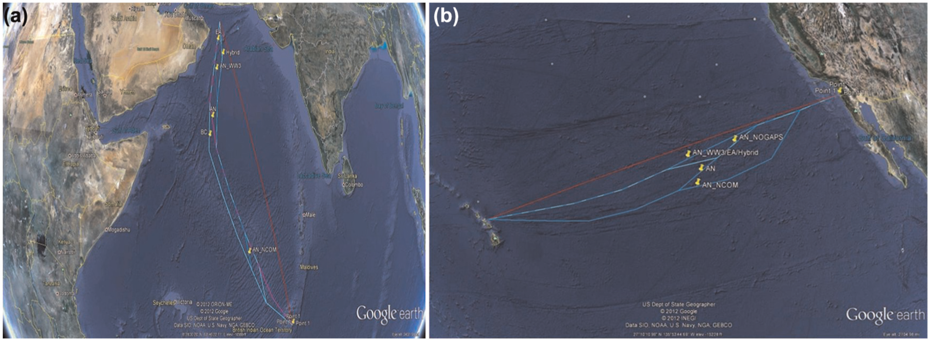
Examples of ship routes for (a) Case-1, (b) Case-2, with the red color denoting the great circle route.

7.2. Fuel-saving characteristics

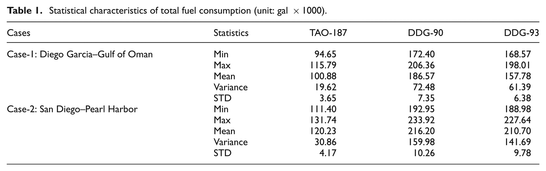
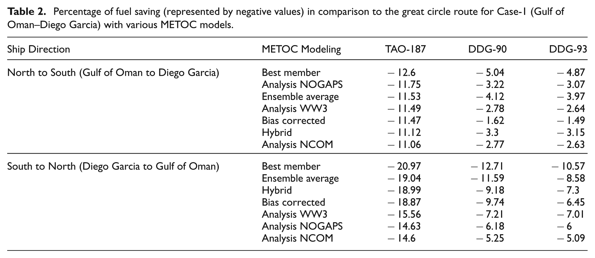
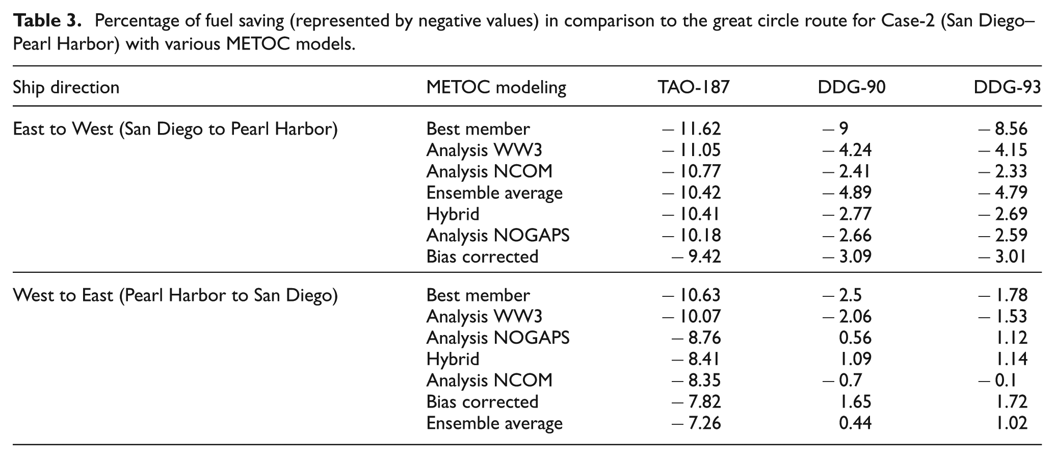
In order to visualize the various route costs by using ensembles, a customized display methodology was developed, which displays all ensembles in a horizontal rank order (Figure 7). Although the difference between ensemble mean (20,686 gal) versus GC (21,229 Gal) is only 2.5%, an overall picture can be derived concerning how well the initial ensemble spread predicted the overall actual weather outcome and route costs. This is observed by viewing the overall blue horizontal bar layout (predicted route cost) in relation to the green horizontal bar layout (predicted route run in the analysis environment cost). Observations identified that sometimes initial ensemble spreads predicted the overall actual route cost spread, and at other times, it under predicts or over predicts the cost. This is a characteristic that is also seen in environmental forecast ensembles when compared with analysis results. Figure 7 clearly shows that the ship route using the METOC ensemble forecasts can save fuel consumption drastically in comparison to the GC route. The statistical characteristics of the total fuel consumption for the three ships (Table 1) shows opportunities using METOC information to save fuels. For example, the difference between maximum and minimum values of TAO-187 is 21,140 gal for Case-1 and 20,340 gal for Case-2. The percentage of fuel saving depends on ship route direction and can reach 12.6% from the Gulf of Oman to Diego Garcia, 21.0% from Diego Garcia to the Gulf of Oman (Case-1, Table 2), 11.6% from San Diego to Pearl Harbor, and 10.6% from Pearl Harbor to San Diego (Case-2, Table 3). Seasons had a profound effect on the route variances as identified by reviewing the outputs from spring, summer, fall and winter runs.

Figure 7.

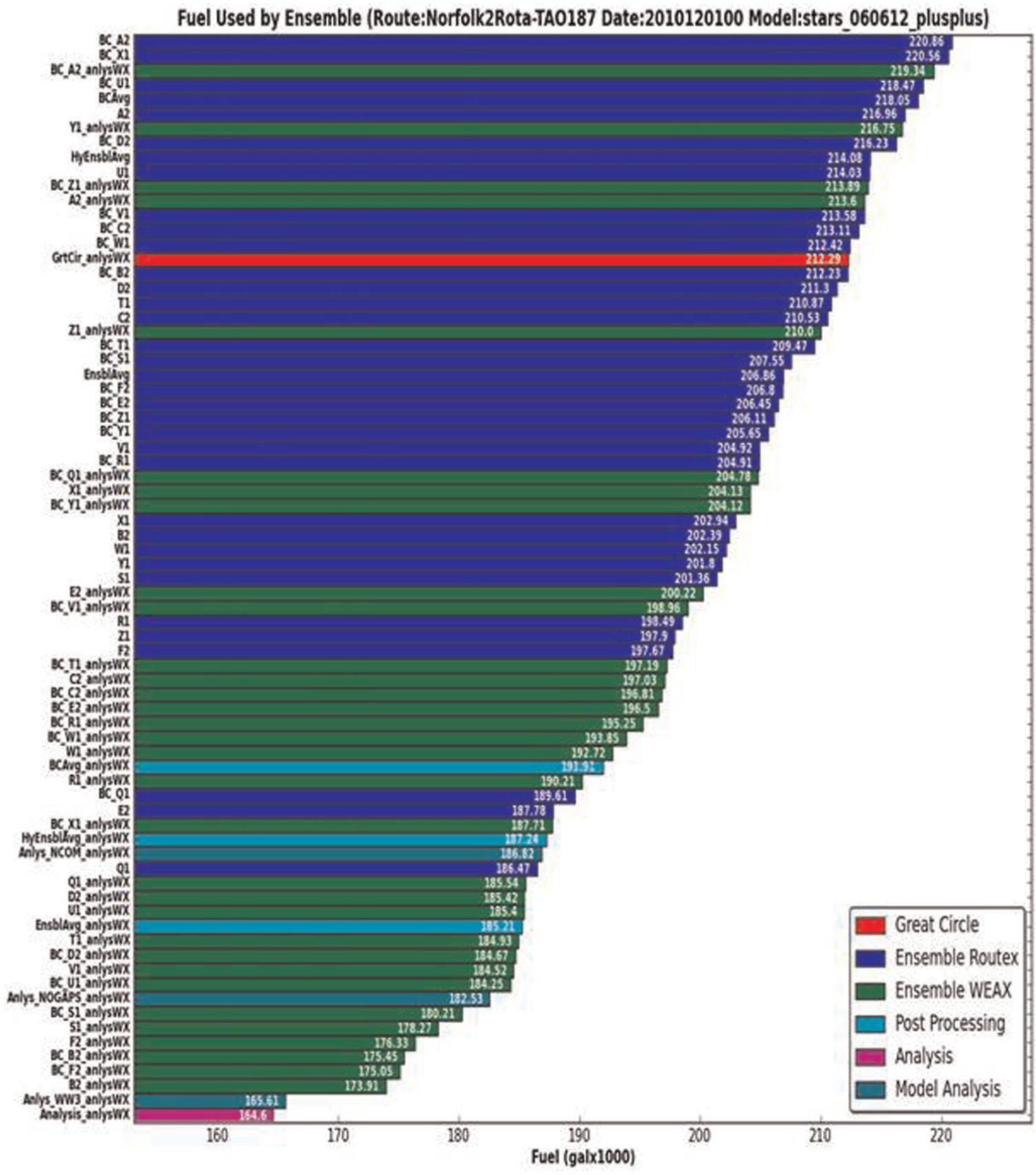
TAO-187 fuel used by ensemble spread distribution (Norfolk to Rota: 01 Dec 2010). Here, the ‘analysis’ bar represent the idea case with the nowcast values (near realistic) for the environmental parameters such as winds, seas, and currents.

Table 1.

Statistical characteristics of total fuel consumption (unit: gal ×1000).

Cases	Statistics	TAO-187	DDG-90	DDG-93
Case-1: Diego Garcia–Gulf of Oman	Min	94.65	172.40	168.57
	Max	115.79	206.36	198.01
	Mean	100.88	186.57	157.78
	Variance	19.62	72.48	61.39
	STD	3.65	7.35	6.38
Case-2: San Diego–Pearl Harbor	Min	111.40	192.95	188.98
	Max	131.74	233.92	227.64
	Mean	120.23	216.20	210.70
	Variance	30.86	159.98	141.69
	STD	4.17	10.26	9.78

Table 2.

Percentage of fuel saving (represented by negative values) in comparison to the great circle route for Case-1 (Gulf of Oman–Diego Garcia) with various METOC models.

Ship Direction	METOC Modeling	TAO-187	DDG-90	DDG-93
North to South (Gulf of Oman to Diego Garcia)	Best member	−12.6	−5.04	−4.87
	Analysis NOGAPS	−11.75	−3.22	−3.07
	Ensemble average	−11.53	−4.12	−3.97
	Analysis WW3	−11.49	−2.78	−2.64
	Bias corrected	−11.47	−1.62	−1.49
	Hybrid	−11.12	−3.3	−3.15
	Analysis NCOM	−11.06	−2.77	−2.63

South to North (Diego Garcia to Gulf of Oman)	Best member	−20.97	−12.71	−10.57
	Ensemble average	−19.04	−11.59	−8.58
	Hybrid	−18.99	−9.18	−7.3
	Bias corrected	−18.87	−9.74	−6.45
	Analysis WW3	−15.56	−7.21	−7.01
	Analysis NOGAPS	−14.63	−6.18	−6
	Analysis NCOM	−14.6	−5.25	−5.09

Table 3.

Percentage of fuel saving (represented by negative values) in comparison to the great circle route for Case-2 (San Diego–Pearl Harbor) with various METOC models.

Ship direction	METOC modeling	TAO-187	DDG-90	DDG-93
East to West (San Diego to Pearl Harbor)	Best member	−11.62	−9	−8.56
	Analysis WW3	−11.05	−4.24	−4.15
	Analysis NCOM	−10.77	−2.41	−2.33
	Ensemble average	−10.42	−4.89	−4.79
	Hybrid	−10.41	−2.77	−2.69
	Analysis NOGAPS	−10.18	−2.66	−2.59
	Bias corrected	−9.42	−3.09	−3.01

West to East (Pearl Harbor to San Diego)	Best member	−10.63	−2.5	−1.78
	Analysis WW3	−10.07	−2.06	−1.53
	Analysis NOGAPS	−8.76	0.56	1.12
	Hybrid	−8.41	1.09	1.14
	Analysis NCOM	−8.35	−0.7	−0.1
	Bias corrected	−7.82	1.65	1.72
	Ensemble average	−7.26	0.44	1.02

Using the GC route as a baseline, some routes would display a clear geometric east of GC route bias during the summer season and a west of GC bias during the winter season. There was a very obvious variance among the various hull classes and propulsion types used. To be as efficient as possible, the SVP tactical decision aid (TDA) needs to be carefully tuned based on the specific hull form, optimum ship speeds and advantageous propulsion plant lineups. An example of this was identified with the TAO, which used significantly less fuel than the gas turbine powered warships were projected to use. This was most likely due to the linearly increasing fuel use curve that characterizes the TAO diesel power curves versus the nonlinear bowl shaped fuel curve used in the GT ships. Additionally, diesel engines are in general more fuel efficient than gas turbine engines.

Fouling slows down a ship and utilizes more fuel for a given route and speed using the GC route as a reference. The SVP model can also identify the environmental impact on fuel saving with various hull clean levels. The interesting finding was that, on average, the SVP route for a hull with more fouling was able to generate an increased relative fuel savings by approximately 1%. This finding was identified by using the DDG-90 vs. DDG-93 class data-stores as inputs for the various experiments (e.g., see Table 2 and Table 3). The only exception to this finding was during periods of heavy weather where the cleaner DDG-93 hull appeared to perform marginally better. This was apparent in the Norfolk to Rota routes where the optimizer had to increase ship speed to avoid heavy weather. The DDG-90 data-store modeled hull and propeller cleaning 6 months before DDG-93; therefore, DDG-90 should have increased fouling, inducing a greater friction cost. The gas turbine ships also displayed sensitivity to both low and high speeds due to their bowl shaped fuel curves. Therefore, if the TDA were to slow the ships to below the speed where fuel consumption increases markedly, a severe fuel cost penalty could be incurred similar to traveling at too high a speed. However, the DDG’s were also relatively slightly more efficient compared to the TAO at higher speeds. Based on the TDA’s spatial discretized resolution, it seems to make sense that longer route length (2500 nm and greater) would suit this TDA better to enable the best chance at a more fuel efficient route. However, relatively shorter runs (around 1500 nm) also displayed noticeable improvements in some of the latitude test cases; therefore, only utilizing transoceanic SVP routes may not be necessary to in order to save fuel.

8. Test for operational fleet use

A Naval Sea System Command (NAVSEA) integrated program team tested the SVPDA tool for operational fleet use and concept of operations (CONOPS) for the USS Princeton CG-59 in an operational demonstration for sea trial test following the 2012 RIMPAC exercises. This effort was part of the Navy’s surface ship energy conservation program initiative.

8.1. Conduct of the test

A data collection and analysis plan (DCAP) was developed in conjunction with Military Sealift Command (MSC) engineering staff to support this test, who embarked on the USS Princeton in Pearl Harbor, HI, and sailed with the ship back to its home port in San Diego on a 6 day voyage. To support testing, communications were established via email, chat, and plain old telephone system (POTS) lines. A movement report (MOVEREP) was generated by the ship and was the mechanism used to obtain a SVP route. Once, the MOVEREP was received by Fleet Weather System (FWC), San Diego, the request was then sent to NRL, Monterey for processing on the SVPDA model. The output route was then sent back to FWC, San Diego and finally sent back to the ship. Once the smart voyage route was received by the ship, the way points and speeds were entered into the electronic chart display and information system – Navy (ECDIS-N) system. After verification by the ship’s Navigator and chain of command, the ship began sailing the SVP route. This process is graphically displayed in Figure 8. Engineering, navigation and environmental logs were taken by the crew throughout the voyage for future analysis. During the cruise, various events occurred which required modification to the SVP route. The above process was then repeated as necessary to obtain new SVP routes.

Figure 8.

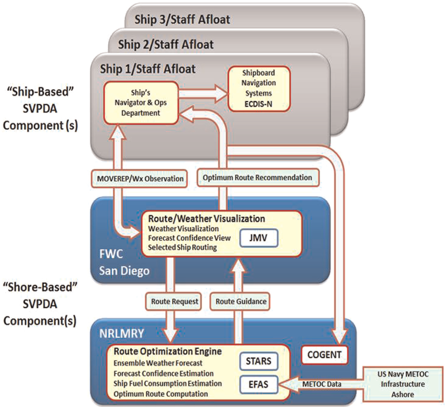
Ship to shore CONOPS for the USS Princeton SVP sea trial.

8.2. Recommendations

The original SVP was created from the ship’s departure port berthing area to the arrival port berthing area. However, most if not all SVP routes should begin at the departure port marker and end at the arrival port marker. Before this point for departure and after this point for arrival, the Navigator will have full control of the ship’s route due to the control of tugs, numerous hazards to navigation, and speed limit constraints experienced while departing and entering ports. Also, the initial SVP route received by the ship contained over 60 waypoints. Currently ships must enter these waypoints manually in the ECDIS-N systems and this is somewhat of an arduous process with that number of points. Until an automated process is established, the routes should be smoothed as much as practical so as not to interfere with saving fuel or compromising ship safety. The waypoints were also received in a format incompatible with the current ECDIS-N system, so a script was written on the shore side to correct the latitude/longitude formatting. CONOPS should be developed to import the SVP directly as a voyage plan into the voyage management system (VMS). This would alleviate the task of entering numerous waypoints into the system and minimize the possibility of manual entry errors.

The DCAP test plan proved to be easy to follow by the crew. It was written in a somewhat generic manner so that it can be executed with minimal training and on multiple ship platform types. Once the SVP was entered into the ship’s ECDIS-N system, it was relatively easy to execute and sail. Logs were collected on a daily basis from the engineering and navigation personnel. Some minor adjustments to the electronic format logs were required based on the ship specific machinery, but this was expected and relatively easy to update after the principle department heads provided feedback. The deck log should be utilized to identify when a SVP route begins/ends or if the ship is deviating from the SVP route, along with the reason.

The first operational change that required an updated SVP route occurred when the ship had a training evolution change for a required exercise. For this exercise, the ship required two new routes, since the Commanding Officer (CO) required two options with different latitudes and longitudes. For future SVPDA CONOPS planning, it’s feasible that multiple routes could be requested by a ship. (e.g. initial, followed by a change from operational tasking/mechanical failure/underway replenishment change) or a CO may just need to have flexibility based on later decision points. During processing with one of the submitted routes, it was discovered that the maximum speed was not high enough to get from point A to point B within the allotted time specified. Therefore, the operational version of STARS should contain some form of error checking to perform a quality assurance (QA) check for this type of erroneous request. It should then inform the operator of the problem and suggest a higher speed or increase of time. Another possibility is that SVPDA would provide the operator a best route, but note that time has been lengthened to account for given maximum speed constraints. The ship’s maximum speed may vary based on propulsion plant line-ups, maintenance and mechanical issues. For propulsion plant line-ups, maximum speed may also be constrained so that the ship can run in trail shaft mode. This mode is only available up to a certain speed and can provide a significant fuel efficiency advantage with this change alone. Therefore, the SVP engine needs to be optimized to provide speed limits based on the propulsion plant efficiency capabilities or reduced capabilities (i.e. trail shaft or split plant ops only). For example, one of the routes run during the CONOPS trial required the ship to travel 18 kts for 90% of the voyage, but then slow at the end. However if the ship could have made the entire route at 17 kts in trail shaft mode, significant fuel savings could have been observed.

Overall the communication process went well with ship to shore connectivity on non-classified and classified email, chat, POTS and normal message traffic. Daily logs that were recorded were sent off the ship via classified email once every two days to a shore side repository. A list of ship operations which would affect the ship being able to follow the SVP route were examined and actually encountered during this CONOPS trial. There were times when the ship had to stop executing the SVP or pause and then request an update based on its current lat/long position. This process worked fairly seamlessly with the only limit being the round trip time that it took to request a new route, received it and entered the update into the ECDIS-N system. On average, this process took approximately 2 hours. A lesson learned from this evolution was that the ship should dead reckon 2 hours down track and use this lat/long for the starting point of the newly requested SVP route due to the round trip delay time. This enabled the ship to begin sailing the new SVP route approximately at the same time that it had been entered into the system.

FNMOC helped develop a useful decision aid which enabled importing the SVP routes and weather into a SIPRnet Google Earth application. Utilizing this tool, shipboard personnel were able to view an entire SVP route with overlaid weather. It was then possible to simulate sailing the ship down track in the future with the weather evolving each day. This tool enabled the CO and ship’s senior leadership to quickly obtain situational awareness as to why a route was possibly zigging to avoid weather or slowing the Speed of Advance to minimize the effects of strong head seas, or to possibly take advantage of strong following seas. The navigator and CO could also use this tool to quickly view SVP routes before entering into the ships ECDIS-N system. After reviewing the history from this tool, there was value in obtaining updated SVP routes every day or at least every other day, as the weather changed noticeably over the course of 4 days compared to what was initially predicted off the coast of the Western U.S.

8.3. Limitations

The first limitation of this test was due to good weather, in that the effects of winds, waves, and currents were not evident in this situation. The GC route was essentially identified, although many valuable CONOPS lessons were learned and best practices were discovered. It would have been a little more satisfying to see that environmental (ensemble model) input to the SVPDA software resulted in at least some change to the GC route that was inevitably used to execute the USS Princeton’s transit to San Diego (along with a percentage of fuel savings, again, as shown in the sensitivity analysis).

The second limitation was due to the fact that the ensemble members were randomly generated in the FNMOC ensemble forecast. It was difficult to identify which member was the best for a long voyage. The bias correction over the past 30 days on one particular member could not be applied into the future. Since the fuel consumption was a highly nonlinear function of the wind speed, direction, wave height, period and direction, pre-processing the ensemble mean value as input to compute the mean value of the fuel consumption might not be suitable in the optimization. There is also a risk of encountering severe sea states because of the averaging process.

8.4. Future work

Unlike a METOC forecast for a fix location with temporal evolution, optimal ship routing involves both temporal and spatial processes. The emphasis of using the ensemble forecast should be on quantifying the risks and their impact on route selection, rather than trying to improve the forecast accuracy into the future based on past performance. Future route optimization for fuel saving will be conducted in three steps with the same departure and arrival times of a voyage. First, the SVP model with the analysis of winds, waves, and currents is taken as the bench mark (100%) of what can be achieved in fuel consumption without the forecast errors, and will be used for comparisons. Second, the route is optimized with forecast weather at departure time. The ship will be moved to the next day along the optimal route and re-optimized again using the archived forecast environmental data. This is repeated until the ship arrives. The phantom route then consists of the positions along the optimal route updated each day. This route is then simulated again with the analysis environmental condition. The fuel increase over the bench mark can be attributed to the forecast uncertainties. Third, the ensemble weather (i.e. mean, bias corrected, hybrid etc.) is used to replace the nominal forecasts in the above bench mark process to see if any techniques in using the ensemble forecast will reduce the fuel consumption over the bench mark one. It is noted that the above process will default to the GC route (minimum distance) and minimum speed route in good weather, but will deviate from the GC route to avoid bad weather similar to taking advice from the Navy’s METOC centers. Such a comparison is more realistic than comparing with the GC route regardless of weather conditions.

9. Conclusions

The primary goal of this study was to assess the impact and sensitivity of METOC input parameters to SVPDA modeling. Ensemble modeling was used to quantify the environmental model uncertainties. We demonstrated that inclusion of realistic METOC environment and platform characteristics into SVPDA would result in fuel reduction for various classes of Navy vessels. It was found that the SVPDA model was very sensitive to the following factors: location, direction, seasonal synoptic/mesoscale weather, hull/propulsion type and condition, route length, specific model improvements, and ensemble methods. Large fuel cost reduction was also identified by utilizing the best ensemble member with the maximum fuel-saving of 20%. Processing time with the SVPDA using multiple ensembles can easily be sped up by running parallel execution processes. During conduct of the CONOPS trial onboard the USS Princeton, we determined and experienced various types of operations which could affect a combatant vessel in conducting a SVP route. Key lessons were learned, while best practices and recommendations were also gained during the conduct of this operational trial. Since the test conducted during the RIMPAC exercise was mostly in good weather with little forecast uncertainties, further investigations are needed to validate the advantage of using ensemble forecast over the nominal forecast in different weather conditions with high forecast uncertainties.

Footnotes

Appendix

Acknowledgements

We thank the Naval Sea System Command (NAVSEA) and the entire SVPDA integrated program team for assisting with prototype development and testing at sea.

Declaration of conflicting interest

The authors declare that there is no conflict of interest.

Funding

This work was supported by the Commander, Naval Meteorology and Oceanography Command, the Naval Research Laboratory, the Naval Oceanographic Office, and the Naval Postgraduate School.

Author biographies

Peter C Chu is a distinguished professor, head of the Naval Ocean Analysis and Prediction Laboratory, and Chair of the Department of Oceanography at the US Naval Postgraduate School.

Scott E Miller is a Lieutenant Commander (USN) at the US Naval Postgraduate School.

James A Hansen is a meteorologist and head of the Meteorological Applications Development Branch at the Naval Research Laboratory, Monterey, California.

References

Chang

Tseng

Chen

. Ship routing utilizing strong ocean currents. J Navig 2013; 60: doi:10.1017/S0373463313000441.

Avgouleas

. Optimal ship routing. Master’s Thesis, Massachusetts Institute of Technology, Cambridge, MA, 2008.

Tolman

. User manual and system documentation of WaveWatch III version 3.14. Technical report no. 276, NOAA/NWS/NCEP/MMAB, 2009.

Martin

. Description of the Navy Coastal Ocean Model version 1.0. Technical report no FR/7322–00–9962, Naval Research Lab, Stennis Space Center, 2000.

Barron

Kara

Martin

. Formulation, implementation and examination of vertical coordinate choices in the global Navy Coastal Ocean Model (NCOM). Ocean Model 2006; 11: 347–375.

Chu

Chen

. Evaluation of the Princeton ocean model using the South China Sea monsoon experiment (SCSMEX) data. J Atmos Oceanic Technol 2001; 18: 1521–1539.

Rhodes

Hurlburt

Wallcraft

. Navy real-time global modeling systems. Oceanography 2002; 15: 29–43.

Fox

Teague

Barron

. The modular ocean data analysis system (MODAS). J Atmos Oceanic Technol 2002; 19: 240–252.

Chu

Wang

Fan

. Evaluation of the US Navy’s modular ocean data assimilation system (MODAS) using the South China Sea monsoon experiment (SCSMEX) data. J Oceanogr 2004; 60: 1007–1021.

10.

Chu

. Two kinds of predictability in Lorenz system. J Atmos Sci 1999; 56: 1427–1432.

11.

Chen

. A dynamic program for minimum cost ship routing under uncertainty. PhD Dissertation, Massachusetts Institute of Technology, Cambridge, MA, 1978.

12.

Chen

Cardone

Lacey

. Use of operation support information technology to increase ship safety and efficiency. Trans Soc Naval Architects Mar Eng 1998; 106: 105–127.

13.

Ballou

Chen

Homer

. Advanced methods of optimizing ship operations to deduce emissions detrimental to climate change. In: MTS/IEEE OCEANS 08 Conference, Quebec City, Canada, 15–18 September 2008, p.12.

14.

Miller

. Smart voyage planning model sensitivity analysis using ocean and atmospheric models including ensemble methods. Master’s Thesis, Naval Postgraduate School, 2012.