Modeling decoy state Quantum Key Distribution systems

Abstract

Quantum Key Distribution (QKD) is an innovative technology which exploits the laws of quantum physics to generate and distribute shared secret key for use in cryptographic devices. Quantum Key Distribution offers the advantage of ‘unconditionally secure’ key generation with the unique ability to detect eavesdropping on the key distribution channel and shows promise for high-security applications such as those found in banking, government, and military environments. However, Quantum Key Distribution is a nascent technology where realized systems suffer from implementation non-idealities, which may significantly impact system performance and security. In this article, we discuss the modeling of a decoy state enabled Quantum Key Distribution system built to study the impact of these practical limitations. Specifically, we present a thorough background on the decoy state protocol, detailed discussion of the modeled decoy state enabled Quantum Key Distribution system, and evidence for component and sub-system verification, as well as, multiple examples of system-level validation. Additionally, we bring attention to practical considerations associated with implementing the decoy state protocol security condition gained from these research activities.

Keywords

Quantum Key Distribution decoy state protocol model and simulation system security system performance

1. Introduction

Quantum Key Distribution (QKD) is the most mature application of the quantum information field and is heralded as a revolutionary technology offering the means for two physically separated parties to generate ‘unconditionally secure’¹ cryptographic key. Employing the laws of quantum physics, QKD systems can detect eavesdropping during the key generation process where unauthorized observation of quantum communication necessarily induces measurable errors. This work builds upon previous work,^1,2,3 with additional details regarding the modeling and simulation of a decoy state enabled QKD system. For detailed treatments and comprehensive reviews of QKD please see Gisin et al.,⁴ Scarani,⁵ Loepp and Wooters⁶ and Nielsen and Chuang.⁷

QKD technology is emerging as an important development in the military and national defense cybersecurity solution space with research occurring in the United States Navy,⁸ Army,⁹ and Air Force.¹⁰ Increasingly practical systems have been realized in numerous experiments and have recently become available from commercial vendors such as ID Quantique (Switzerland),¹¹ SeQureNet (France),¹² Quintessence Labs (Australia),¹³ MagiQ Technologies (USA),¹⁴ and Quantum Communication Technology Co., Ltd. (China).¹⁵ However, QKD is a nascent technology where real-world systems are constructed from non-ideal components, which may significantly impact system performance and security. As with any new technological development, and especially security technologies, one must carefully evaluate its use holistically. In the case of QKD systems, its overall security posture relies not only upon its theoretical security proofs but upon how well they are realized (i.e., designed, implemented, and operated), which few have addressed.

In this article, we provide a review of the decoy state protocol and describe our decoy state enabled QKD system model built to study practical system implementation issues. Furthermore, we provide results supporting component and sub-system verification, as well as, system-level validation against eight experimental systems. Through these exercises we gain confidence in the subject model, as well as, additional insight into design, implementation, and operational considerations for the decoy state protocol security condition.

A comprehensive discussion of the decoy state protocol is provided in Section 2, which includes a discussion of multi-photon vulnerabilities associated with practical QKD realizations. The modeled decoy state enabled QKD system is described in Section 3, with emphasis on the end-to-end quantum communications. A discussion of component and sub-system verification, along with system-level validation activities and their results are provided in Section 4. Practical implementation considerations for the decoy state security condition are introduced in Section 5. Conclusions and future works are offered in Section 6.

2. QKD systems and the decoy state protocol

2.1. QKD Background

The genesis of QKD technology can be traced back to Stephen Wiesner, who first developed the idea of fraud-proof quantum money in the late 1960s.¹⁶ In 1984, Charles Bennett and Gilles Brassard operationalized this concept when they proposed the first QKD protocol (i.e., BB84) where single photons, representing quantum bits (qubits), are used to securely generate shared cryptographic key.¹⁷Figure 1 illustrates a QKD system configured to generate shared secret key K for use in external encryptors to protect sensitive data, voice, or video communications. The architecture consists of a sender ‘Alice’, a receiver ‘Bob’, a quantum channel (i.e., an otherwise unused ‘dark’ optical fiber), and a classical channel (i.e., a conventional networked connection). Alice and Bob each consist of a central processing unit (CPU) configured to control QKD processes, a network interface configured to control communications on the classical channel, and a quantum module configured to control communications on the quantum channel. QKD systems can be paired with traditional symmetric encryption algorithms (e.g., DES, 3DES, or AES) where the QKD-generated key is used to increase the security posture of encrypted communications through frequent re-keying. Alternatively, the QKD-generated key can be used in conjunction with the One-Time-Pad (OTP) encryption algorithm to provide unbreakable communications.^18,19

Figure 1.

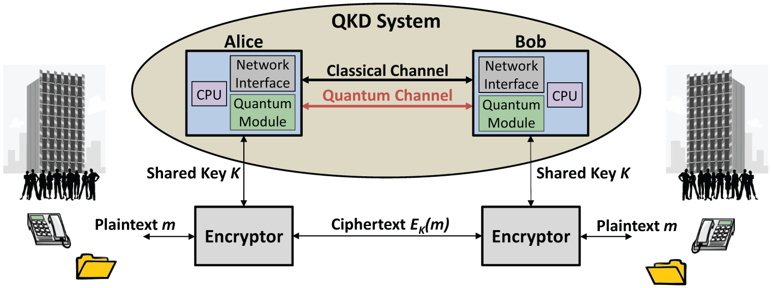
QKD system context diagram. QKD: Quantum Key Distribution.

2.2 The first QKD protocol: BB84

BB84 is a polarization-based prepare and measure QKD protocol, where four polarization states ↔, ↕, ⤡, and ⤢ are used to encode qubits as depicted in Table 1.¹⁷ Alice prepares qubits according to a randomly selected bit value (i.e., ‘0’ or ‘1’) and a randomly selected basis (i.e., rectilinear ‘ ⊕ ’ for the orthogonal polarization pair ↔, ↕ or diagonal ‘ ⊗ ’ for the orthogonal polarization pair ⤡, ⤢). For example, when the bit value ‘0’ and the basis ‘ ⊕ ’ is selected, the qubit is prepared in the horizontal orientation state ↔. Likewise, when the bit value ‘1’ and the basis ‘ ⊗ ’ is selected, the qubit is prepared in the diagonal state ⤢. In this manner, Alice randomly prepares qubits through polarization modulation and sends them to Bob where he randomly selects a basis ( ⊕ or ⊗) to measure each qubit. When Alice’s prepared and Bob’s measured bases agree, the qubit is correctly read with a high probability. Otherwise a random result occurs as depicted in the last column of Table 1 with a 0 or 1. The preparation, transmission, and measurement of qubits between Alice and Bob is known as ‘quantum exchange’ and inherently quantum in nature, whereas the remainder of the BB84 protocol (sifting, error reconciliation, and privacy amplification) is entirely classical.

Table 1.

Polarization-based prepare and measure example.

The sender ‘Alice’ prepares			The receiver ‘Bob’ measures
Random bit value	Random basis	Prepared polarization state	Random basis	Measured bit value
0	⊕	↔	⊕	0
0	⊕	↔	⊗	0 or 1
1	⊕	↕	⊕	1
1	⊕	↕	⊗	0 or 1
0	⊗	⤡	⊕	0 or 1
0	⊗	⤡	⊗	0
1	⊗	⤢	⊕	0 or 1
1	⊗	⤢	⊗	1

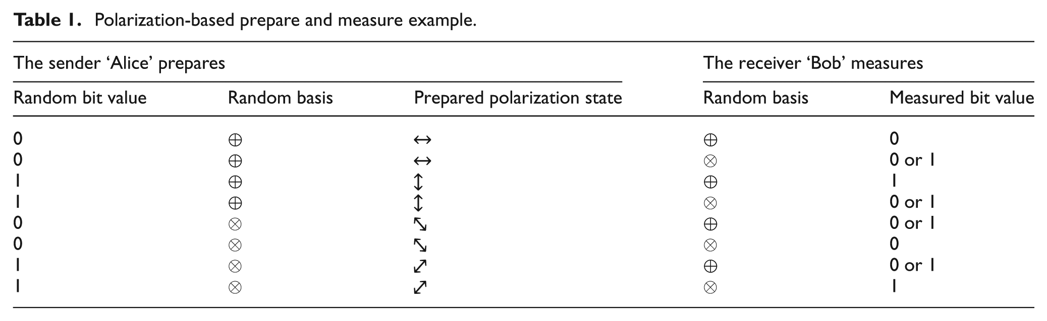
During sifting, error reconciliation, and privacy amplification Alice and Bob use classical information theory techniques and communicate over the classical channel. For sifting, Bob announces the measurement bases he used to Alice, and she responds indicating where the prepared and measured bases agreed (note only the bases are revealed and not the encoded bit values). Due to the random nature of Bob’s measurement basis selection, approximately 50% of the detected qubits are mismatched (i.e., erroneous) and sifted out (i.e., removed) of the secret key. Error reconciliation algorithms perform bi-directional error correction of the shared sifted keys to correct for quantum communication errors, while privacy amplification compensates for information leaked on the classical channel during error correction by producing a smaller, more secure key. Details of these processes can be found in Gisin et al.⁴ and Scarani et al.⁵

2.3 Multi-photon vulnerabilities in realized QKD systems

The security of QKD is based on ‘quantum uncertainty’ inherent in the BB84 protocol, where interference on the quantum channel necessarily increases the Quantum Bit Error Rate (QBER).^4,5 If an eavesdropper, commonly referred to as ‘Eve,’ attempts to listen on the quantum channel, she introduces additional errors and increases the QBER as captured in formal security proofs.^20,21 Since the source of quantum bit errors cannot be known, all errors are attributed to Eve; thus the QBER must be closely monitored. Owing to device imperfections and transmission errors, operational QBERs are typically 3-5% with practical security thresholds <12%.⁵ If the QBER threshold is exceeded, the key generation process is generally aborted, as it is assumed an adversary is interfering with the quantum key exchange.⁵

The unique nature of QKD theory makes it well-suited for high-security applications such as military, banking, and government environments, where information protection is of primary concern. However, practical design and implementation limitations can quickly undermine pristine theoretical security proofs.²² For example, BB84 security proofs assume (and attempt to compensate for) perfect on-demand single photon sources in Alice, yet practical on-demand single photon sources are not currently available nor are they expected in the near-term.²² Therefore, most prepare and measure architectures attenuate a classical laser pulse down from millions of photons to a Mean Photon Number (MPN) of 0.1 according to QKD security practices.⁴ 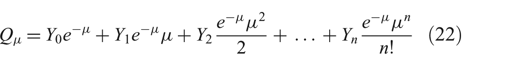These sub-quantum pulses are referred to as ‘weak coherent pulses’ and represented probabilistically using a Poisson distribution, $P (n | λ) = λ^{n} e^{- λ} / n!$ , where $λ = MPN$ and $n$ represents the number of photons in an optical pulse.⁴ For example, when $λ = MPN = 0.1$ , 90.48% of the pulses will have no photons, 9.05% of the pulses will have one photon, and 0.47% of the pulses will have two or more photons. This means only 1 in 10 pulses leaving Alice will actually contain a prepared qubit; the majority of pulses generated by Alice are attenuated to an energy level equivalent to zero photons.

A low MPN results in poor quantum throughput and thus low key generation rates. However, a low MPN is desirable to reduce the likelihood of multi-photon pulses, each of which exposes information about the distributed cryptographic key to a listening adversary. This multi-photon security vulnerability has been subject of a number of attacks against the quantum channel. More specifically, the Photon Number Splitting (PNS) attack was conceived to gain maximum information from this vulnerability without detection.^23–26 The decoy state protocol was introduced to mitigate this attack and has since become widely implemented in several high performance QKD experiments .²⁷

2.4 The decoy state protocol

The decoy state protocol represents a significant advancement in QKD technology, as the protocol is relatively cheap and easy to implement, while simultaneously increasing quantum throughput and security on the quantum channel. The decoy state protocol was introduced in 2003²⁷ and quickly improved in an initial series of works^28–31,38 and later.^{32–37,39,40,41}. Decoy state enabled QKD systems utilize the conventional signal state plus dedicated security states (decoy and vacuum) as described in Table 2. In this three state configuration, the signal state, represented as a ‘ μ,’ facilitates higher key distribution rates and greater operational distances through an increased MPN (i.e., an MPN of 0.6 is greater than the traditionally used 0.1), while the decoy state, represented as a ‘ ν,’ is used to increase the likelihood of detecting an attack using differential statistical analysis. Utilizing different MPNs for the signal and decoy states, allows the QKD system to detect photon number specific interference, such as the PNS attack (described in Section 5). The vacuum state, represented as a ‘ $Y_{0}$ ,’ is used to determine the detector error rate at Bob, where erroneous detections, known as ‘dark counts’ are measured.

Table 2.

Example decoy state protocol configuration.

State	Purpose	MPN	Occurrence percentage
Signal, μ	The signal state is used to transmit quantum pulses used for generating secret key.	0.6	70%
Decoy, ν	The decoy state is used to increase the likelihood of detecting photon number specific interference (i.e., the PNS attack) on the quantum channel through statistical differentiation with the signal state.	0.2	20%
Vacuum, $Y_{0}$	The vacuum state is used to determine the detector dark count rate when no photons are present.	∼0	10%

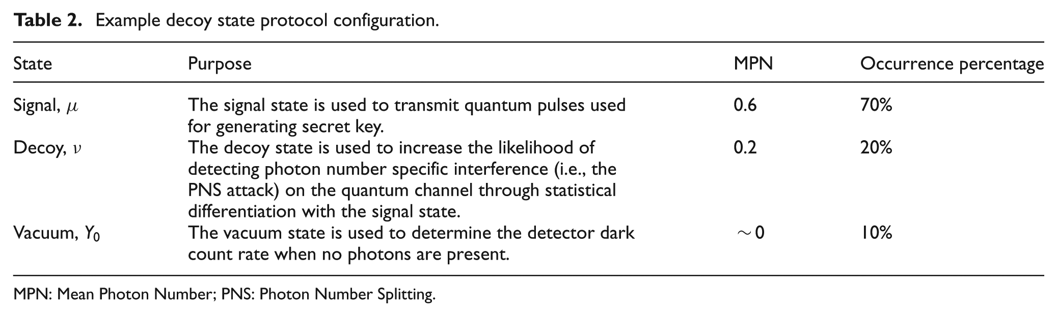
MPN: Mean Photon Number; PNS: Photon Number Splitting.

An outline of the decoy state protocol is described in Table 3^28,30 (note we’ve decomposed the decoy state protocol into multiple steps for clarity; it may be described differently, especially with respect to its implementation). The first step in the protocol is known as quantum exchange, where signal, decoy, and vacuum states are randomly transmitted across the quantum channel according to their unique MPN and occurrence percentage. Each pulse must have identical characteristics (e.g., wavelength, duration, etc.) other than the MPN, such that Eve cannot distinguish a decoy state from a signal or vacuum state.

Table 3.

Decoy state protocol.

Step	Name	Detailed description
1	Quantum exchange	Alice randomly encodes and transmits signal, decoy, and vacuum states (i.e., qubits) based on the prescribed occurrence percentages and MPNs, while Bob measures each qubit. This step is typically described as ‘quantum exchange.’
2	Sifting	Bob announces the basis he used to measure each qubit. Alice responds by announcing which bases are correct, along with the state: signal, decoy, or vacuum for each pulse sent. Alice and Bob perform sifting on both the signal and decoy state qubits for matched bases.
3	Count decoy state errors	For the sifted decoy state qubits, Alice announces the encoded bit values to Bob over the classical channel. Bob performs a comparison of Alice’s prepared bits and his measured values, and records the number of errors for use in step 5.
4	Signal state error reconciliation	For the sifted signal state qubits, Alice and Bob perform error reconciliation where quantum communication errors are counted and corrected for using bi-directional error correction algorithms over the classical channel. The number of corrected errors is recorded for use in step 5.
5	Calculate Gains, QBERs, and Dark Counts	The signal gain $Q_{μ}$ and decoy gain $Q_{ν}$ , respectively, are calculated from the measured number of qubits and total number of pulses sent. The signal QBER $E_{μ}$ is calculated from the measured number of errors in the reconciled key and the number of sifted signal states, while the decoy state QBER $E_{ν}$ is calculated from the measured number of errors in the sifted decoy state qubits. The number of detections measured by Bob when Alice sent a vacuum states is used to determine the system’s dark count probability $Y_{0}$ .
6	Perform decoy state security check	A comparison of signal and decoy estimated photon number specific yields $Y_{n}^{siganl}$ , $Y_{n}^{decoy}$ and/or QBERs $e_{n}^{signal}$ , $e_{n}^{decoy}$ is performed. If they are not the same (i.e., within a predetermined tolerance), an eavesdropper is assumed to be listening on the quantum channel and the key is considered compromised.

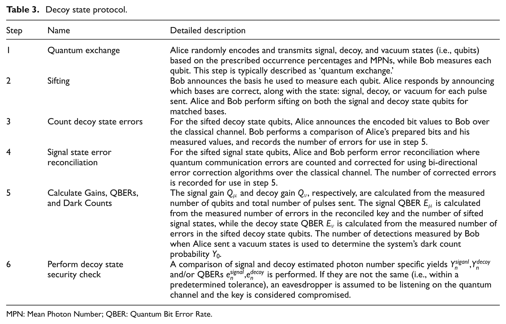
MPN: Mean Photon Number; QBER: Quantum Bit Error Rate.

After quantum exchange, Alice and Bob perform sifting where they announce the bases used to prepare and measure qubits along with each qubit’s state (signal, decoy, or vacuum). For the signal and decoy states, non-matching bases are sifted from the raw secret key, where the correctly matched signal states contribute to a sifted secret key and the decoy states are used for security analysis. Sifting is not necessary on vacuum states, since every detection is a dark count regardless of the basis.

Steps 3 and 4 are responsible for identifying, counting, and correcting errors in the signal and decoy state transmission. Counting of decoy state errors is accomplished by publically announcing and comparing the prepared and measured bit values, while error reconciliation techniques such as winnow, cascade, or low density parity check are used to perform bi-directional error correction of Alice’s and Bob’s sifted signal qubits without revealing specific bit values.^4,5

In step 5, a number of decoy state protocol unique calculations are made from performance measurements: the signal gain $Q_{μ}$ is the ratio of Bob’s signal detections to Alice’s number of signals pulses sent; the decoy gain $Q_{ν}$ is the ratio of Bob’s decoy detections to Alice’s number of decoy pulses sent; the signal QBER $E_{μ}$ is the ratio of errors in the signal state to the number of sifted signal pulses; the decoy QBER $E_{ν}$ is the ratio of errors in the decoy state to the number of sifted decoy pulses; and the dark count yield $Y_{0}$ is the ratio of Bob’s erroneous detections to Alice’s total number of vacuum pulses sent (detailed treatment of these measurements is provided in Section 2.5). Step 6 is responsible for executing the decoy state security condition which ensures there is no unauthorized interference on the quantum channel. The security check is conducted through differential statistical analysis, described in Section 5.

2.5. Secret key rate

QKD systems are designed to securely distribute cryptographic key; however, due to higher MPNs (and therefore more multi-photon pulses) associated with the decoy state protocol, it is important to limit the secret key rate to pulses originating from Alice with a single photon. This relationship is captured in the secret key rate.^21,28,30

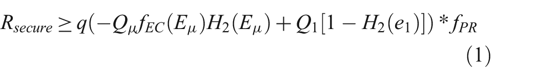
R_{s e c u r e} \geq q (- Q_{μ} f_{E C} (E_{μ}) H_{2} (E_{μ}) + Q_{1} [1 - H_{2} (e_{1})]) * f_{P R}

(1)

where the parameters are described in Table 4.^28,30 Of note, much of the initial decoy state research focused on increasing the secure key rate by providing improved bounds for the single photon gain $Q_{1}$ and the single photon QBER $e_{1}$ . Specifically, the single photon gain $Q_{1}$ should be maximized while the single photon QBER $e_{1}$ is minimized. However, in practical QKD system implementations (i.e., those with classical laser sources), the number of single photon pulses originating from Alice is directly correlated to the number of unsecure multi-photon pulses. Thus there is a tradeoff between performance (i.e., signal gain) and security (i.e., the number of multi-photon pulses).

Table 4.

Secret key rate parameters.^28,30

Secret Key Rate Parameter	Parameter definition	Parameter description or calculation
$f_{PR}$	laser pulse rate measured in Hz.	Typical laser pulse rates are 2–5 MHz. However, the pulse rate may vary greatly depending upon the QKD system design and implementation.
$q$	protocol efficiency fraction is calculated from system measurements.	$q = \frac{Number of bits in error reconciled key}{Total number of detected signal pulses}$
$Q_{μ}$	gain of the signal state is calculated from system measurements. The decoy state gain $Q_{ν}$ is similarly calculated.	$Q_{μ} = \frac{Number of signal detections}{Total number of sent signal pulses}$
$E_{μ}$	QBER of the signal state is calculated from system measurements. The decoy state QBER $E_{ν}$ is similarly calculated.	$E_{μ} = \frac{Number of signal bits errors}{Number of bits in error reconciled key}$
$f_{EC} (E_{μ})$	error reconciliation efficiency is determine from [42] based on the signal state QBER $E_{μ}$ from equation (5).	The error reconciliation efficiency varies dependent upon the signal state QBER. Typical values are $\leq 1.15$ for QBERs $\leq 1.15$ .
$H_{2} (E_{μ})$	uncertainty in the signal state QBER is calculated using Shannon’s binary entropy limit [19] based on the QBER $E_{μ}$ from equation (5).	$H_{2} (E_{μ}) = - E_{μ} \log_{2} (E_{μ}) - (1 - E_{μ}) \log_{2} (1 - E_{μ})$
$Q_{1}$	estimated gain of pulses originating from Alice with one photon is calculated from system operational parameters (signal and decoy MPNs μ and ν), the gain $Q_{μ}$ from equation (4), and supporting equations (12–14).	$Q_{1} \geq Q_{1}^{Lower} = \frac{μ^{2} e^{- μ}}{μ ν - ν^{2}} (Q_{ν}^{Lower} e^{ν} - Q_{μ} e^{μ} \frac{ν^{2}}{μ^{2}} - Y_{0}^{Upper} \frac{μ^{2} - ν^{2}}{μ^{2}})$
$H_{2} (e_{1})$	uncertainty in the signal QBER for pulses originating from Alice with one photon is calculated using Shannon’s binary entropy limit¹⁹ based on the single photon QBER $e_{1}$ from equation (10).	$H_{2} (e_{1}) = - e_{1} \log_{2} (e_{1}) - (1 - e_{1}) \log_{2} (1 - e_{1})$
$e_{1}$	estimated QBER of pulses originating from Alice with one photon is calculated from system operational parameters (signal MPN μ), the gain $Q_{μ}$ from equation (4), the QBER $E_{μ}$ from equation (5), the dark count error rate $e_{0} = \frac{1}{2}$ , and supporting equations (12) and (14).	$e_{1} \leq e_{1}^{Upper} = \frac{E_{μ} Q_{μ} - e_{0} Y_{0}^{Lower} e^{- μ}}{Q_{1}^{Lower}}$
$Y_{0}$	dark count is calculated from systems measurements.	$Y_{0} = \frac{Number of dark count detections}{Number of acuum pulses sent}$
$Y_{0}^{Lower}$	estimated lower bound of dark count probability is calculated from system measurements for 10 standard deviations, where $N_{0}$ is the number of vacuum pulses sent by Alice and $Q_{0}$ is the measured vacuum state gain (see equation (4)).	$Y_{0}^{Lower} = Y_{0} (1 - \frac{10}{\sqrt{N_{0} Q_{0}}})$
$Y_{0}^{Upper}$	estimated upper bound of dark count probability is calculated from system measurements for 10 standard deviations, where $N_{0}$ is the number of vacuum pulses sent by Alice and $Q_{0}$ is the measured vacuum state gain (see equation (4)).	$Y_{0}^{Upper} = Y_{0} (1 + \frac{10}{\sqrt{N_{0} Q_{0}}})$
$Q_{ν}^{Lower}$	estimated lower bound of decoy state gain is calculated from system measurements for 10 standard deviations, where $N_{ν}$ is the number of decoy pulses sent by Alice.	$Q_{ν}^{Lower} = Q_{ν} (1 - \frac{10}{\sqrt{N_{ν} Q_{ν}}})$

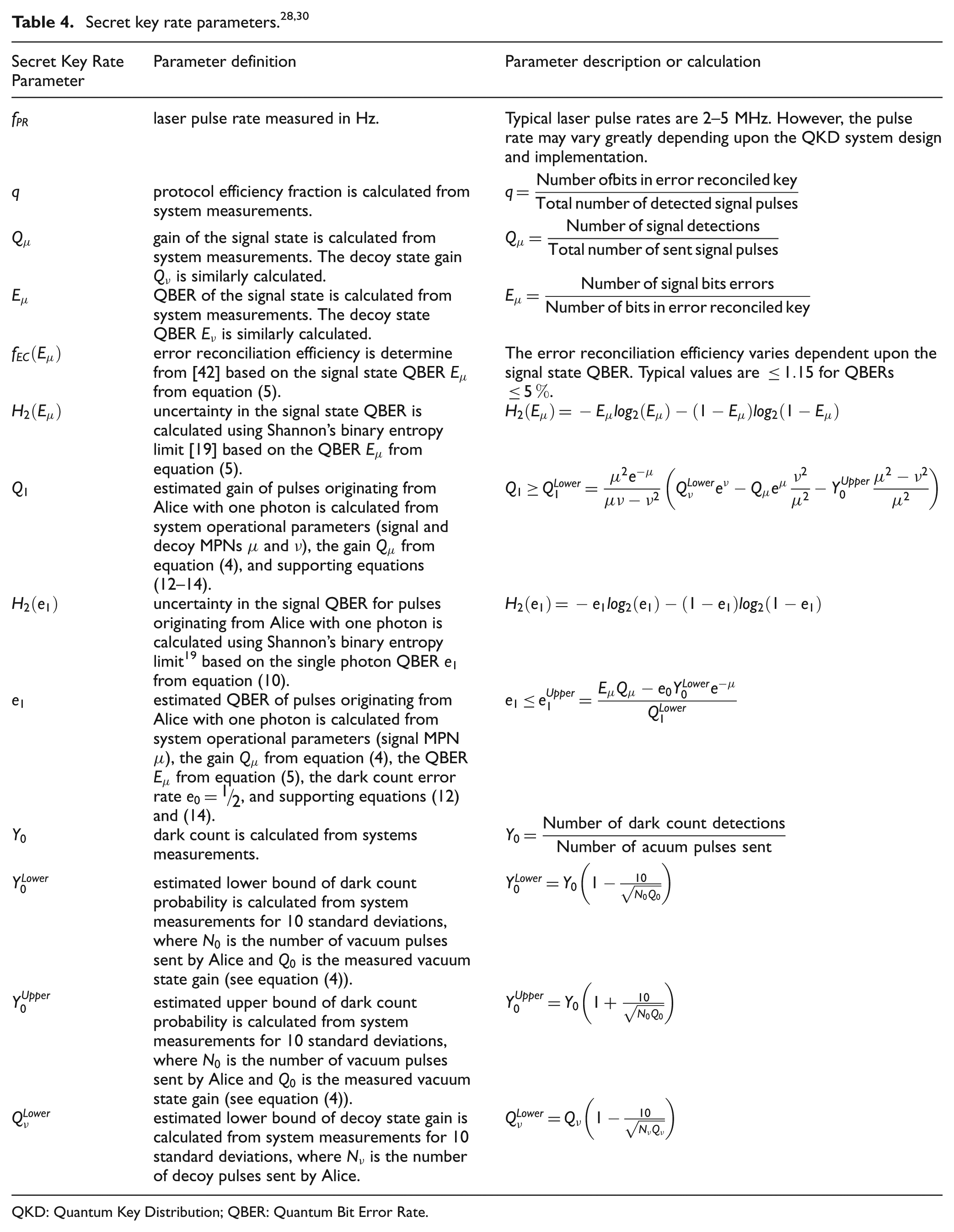
QKD: Quantum Key Distribution; QBER: Quantum Bit Error Rate.

3. The decoy state enabled QKD system model

In this section we describe the decoy state enabled QKD model built to study system performance and security.¹ The model was constructed in a QKD modeling framework using the OMNeT++ Discrete Event Simulation (DES) environment with an extended library of optical components.³ This framework enables models to be built in a modular fashion, supporting multiple levels of abstraction to more efficiently answer performance and security questions. The library consists of 17 optical components modeled in an event-driven paradigm with supporting control logic modeled in a process-based paradigm, see the Appendix of Mailloux et al.³ for details. Each component is configured with 12–15 (and up to 27) configurable parameters.

The focus of this research effort pertains to accurately modeling interactions between system-level behaviors and quantum phenomenon in an end-to-end decoy state quantum communication path. Thus the model is described in three distinct parts: (a) the sender, Alice’s quantum module; (b) the quantum channel; and (c) the receiver, Bob’s quantum module. Modeling assumptions are described below, where appropriate.

3.1. Alice’s quantum module

Figure 2 provides a depiction of Alice’s quantum module (introduced in Figure 1) designed to generate sub-quantum pulses as described in Section 2.2. Alice’s quantum module is designed to generate weak coherent optical pulses at a specified pulse rate, which have the desired MPN and polarization, in a reproducible manner. For example, Alice generates classical laser pulses, randomly selects an encoding basis and bit value, prepares the desired polarization state (↔, ↕, ⤡, or ⤢), and attenuates the pulse’s energy down to the specified MPN.

Figure 2.

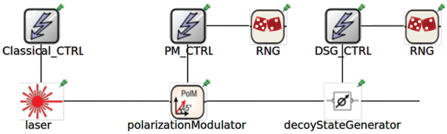
Modeled Alice quantum module. RNG: Random Number Generators.

The module is shown with a classical laser source, a Polarization Modulator (PM), a Decoy State Generator (DSG), two Random Number Generators (RNG), and respective controllers (CTRL). This representation is a simplification of Alice’s quantum module where additional control and timing synchronization components are not of interest in the simulation study and are therefore assumed to operate properly and not shown in the module diagrams. The laser controller is configured to generate classical pulses by triggering the laser to fire in response to an electrical trigger pulse (e.g., 2 Mhz). The laser’s pulse rate is configurable to match any system of interest or experiment with alternative configurations. The laser is designed to generate optical pulses representative of the ID300 commercial laser, including pulse shape, amplitude, duration, and wavelength^11,43 (detailed discussion of the laser pulse is provided in Mailloux et al.⁴⁴). Additionally, variations in the laser pulse can be turned on or off when so desired. The laser generates classical energy light pulses, where the PM prepares (or encodes) each optical pulse according to the random bit and basis provided by the RNG. The modeled RNG can be configured to provide pseudo random numbers through conventional RNG algorithms or quantum random numbers through a dedicated hardware interface.¹¹

The DSG controller randomly selects the state type (i.e., signal, decoy, or vacuum) according to each state’s occurrence percentage and the second RNG. The controller adjusts the DSG to reduce the classical pulse energy down to the specified signal, decoy, and vacuum MPNs as illustrated in Table 2. This behavior is representative of an electronic variable optical attenuator configured to apply 0–30 dB depending on the desired MPN. For example, if the desired state is a signal pulse with an MPN of 0.6, the DSG will apply ~6 dB. For a decoy state of 0.2 MPN, the DSG will apply ~10 dB, and ~30 dB for the vacuum state.

3.2. Quantum channel

The quantum channel is representative of Single Mode Fiber (SMF) where both the length and loss can be easily adjusted. Channel loss is specified per km (e.g., 0.20 dB per km) where the total loss due to fiber length and connectors is expressed as a single value. Alternatively, the loss can be expressed as an efficiency or percentage. For example, losses for a 50 km SMF-28 fiber are $0.20 \frac{dB}{km} * 50 km = 10 dB$ , a 90% loss, or conversely 10% efficiency. The modeled quantum channel is also designed to account for propagation specific phenomenon such as thermal expansion, index of refraction, and chromatic dispersion. Additionally, the modeled channel is capable of simulating the effects of random physical disturbances such as bends in the fiber, vibration, or other instabilities.¹ Regarding propagation through the fiber for the simulations presented here, we assume Alice and Bob have correct basis alignment and timing control for precise photon detection at Bob (i.e., polarization rotation in the quantum channel is ideally corrected and synchronized). Typical misalignment would account for ~1% errors.⁴

3.3. Bob’s quantum module

Figure 3 is a depiction of Bob’s quantum module (introduced in Figure 1) shown with a beamsplitter (BS), a half wave plate, two polarizing beamsplitters (PBS1 and PBS2), four Single Photon Detectors (SPDs), and one controller. Pulses entering Bob are randomly split by the BS (i.e., a 50/50 BS) and transmitted to PBS2 towards the horizontal/vertical SPDs or reflect towards the half wave plate, PBS1, and the diagonal/antidiagonal SPDs. This configuration is commonly referred to as a ‘passive basis selection,’ where Bob’s random basis selection intrinsically occurs at the 50/50 BS. This configuration is generally considered advantageous as it does not require additional RNGs in Bob.

Figure 3.

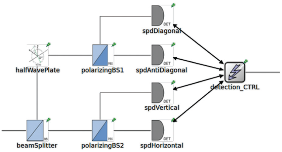
Modeled Bob quantum module.

The PBSs are modeled similarly to the BS; however, they are designed to transform pulses into known orthogonal polarization states (i.e., the horizontal or vertical state) from any input state. More specifically, pulses transmitted by the BS to PBS2, are split into the horizontal state ↔ or vertical state ↕ and sent to their respective SPDs. With respect to pulses reflected by the BS towards PBS1, they receive a $π / 4$ polarization rotation from the half wave plate, which is configured to transform diagonally prepared pulses into the rectilinear basis and propagate toward PBS1. Thus the diagonal and antidiagonal pulses can be correctly measured by their respective SPDs. In this manner, rectilinearly prepared qubits which proceed through PBS2 will be correctly detected at the vertical and horizontal SPDs and diagonally prepared qubits which proceed through PBS1 will be correctly detected at the antidiagonal and diagonal SPDs. Pulses which are sent to the incorrect (i.e., non-matching) measurement basis will result in a random bit value, which is later sifted out from the QKD-generated key. This behavior is represented in Table 1, where the correct bit value is determined when measured in the correct basis and a random result occurs when measured in the wrong basis.

In the modeled architecture, the SPDs are responsible for probabilistically determining the detection of weak coherent pulses; thus simulating the uncertainty inherent in quantum phenomenon.^45,46 Specifically, for each pulse arriving at an SPD a probabilistic determination is made for how many photons arrived according to its MPN and the Poisson distribution.⁴ Note: after propagating through the quantum channel and Bob’s architecture the pulse’s MPN is significantly lower than when it left Alice (e.g., a signal state MPN of 0.65 propagating though 50 km of fiber with 0.20 dB loss per km, and a passive basis selection architecture with 3 dB loss will have an MPN of ~0.0325). This probabilistic design mimics the desired behavior of single photon generation and detection in the modeled architecture.⁴⁷

The detection CTRL is configured to precisely ‘gate’ the SPDs to reduce noise (i.e., dark counts and after pulsing) while detecting single photon pulses. This means the SPDs change from a classical detection state to a heightened ‘Geiger’ state configured to detect the arrival of single photons. Typical gating periods are on the order of nanoseconds (i.e., 10^-9 sec) controlled by the detection controller and assumed to be ideal in this model. Bob’s SPDs take into account detector efficiency (e.g., 10%), dark count probability per gate interval (e.g., 10^-6), detector dead time interval (e.g., 10^-5 sec), after pulsing probability (e.g., 10^-3 with the proper dead time interval), and expected photon arrival times (e.g., 10^-12 sec). Modeling and simulating these parameters provides a baseline for studying the performance and security of realized decoy state QKD systems.

3.4 Decoy state protocol logic

The decoy state protocol as outlined in Table 3 is implemented through the described physical model and control logic within Alice and Bob. In our model, Alice is implemented as the protocol master and Bob as the slave; however, these roles can change depending on how the desired functionality is modeled. In some cases it may be more advantageous to have Bob, as the receiver, control processes or sub-processes to reduce the number of classical communications (and thus reduce the amount of leaked information).

To perform quantum exchange (step 1 of Table 3), Alice and Bob use a flexible data frame structure defined as a classical timing and polarization control reference pulse followed by a configurable number of weak coherent pulses (e.g., 100 or 1000) with adjustable spacing between both frames and pulses. Alice randomly distributes signal, decoy, and vacuum pulses within each frame according to their occurrence percentages and records the frame number, bit position, prepared basis, encoded bit value, and state (signal, decoy, or vacuum) for each pulse generated. Likewise, upon detection Bob stores the frame number, bit position, measurement basis, and detected value. Quantum exchange ends when Bob reaches the specified number of total detections (signal, decoy, and vacuum).

Steps 2–6 of Table 3 are not quantum in nature and occur over the classical channel using abstracted message traffic passed between Alice and Bob including large memory arrays to quickly and easily facilitate information exchange for the remaining classical steps. During sifting (step 2), Bob publicly announces the basis in which he detected each qubit to Alice, and she responds by announcing which bases are correct and identifies the signal, decoy and vacuum states. Alice and Bob perform sifting on both the signal and decoy state detections to identify when they have matching prepare and measure bases. For each decoy state pulse, Alice also announces the encoded bit value to Bob. The announced decoy state bases and bit values are used to calculate the number of errors in the decoy state transmission (Step 3). Additionally, Alice calculates the dark count rate $Y_{0}$ using the total number of detections during vacuum states as defined in Table 4.

Next, Alice and Bob begin error reconciliation (step 4) of the sifted key to correct for quantum communication errors. They first sacrifice an adjustable percentage of the signal state bits (e.g., 25%) to estimate the error rate. This means, Alice randomly chooses the specified percentage of post-sifted signal bits and sends them (frame number, bit number, and value) to Bob. He calculates the estimated error rate and sends it back to Alice. If the estimated error rate is higher than a user defined threshold (e.g., 12%), the protocol is aborted; this is done to conserve processor resources. If the estimated error rate is below the threshold, the QKD system performs error reconciliation. The simulation framework provides the ability to use conventional error reconciliation algorithms such as winnow, cascade, and low density parity check where the algorithm’s efficiency is based on the estimated error rate³. For example, the error rate can be used to determine block correction sizes and influences the number of communications necessary for error reconciliation. Since these algorithms are resource intensive, and not of interest to our simulation study, we implemented a ‘perfect’ error reconciliation algorithm that quickly counts and corrects errors without unnecessary complexity. We anticipate using the perfect error reconciliation most often because of its speed advantage while running large simulation trails. During perfect error reconciliation, Alice sends her key to Bob who determines the number of errors in his key and returns the results back to Alice.

In step 5, the decoy state protocol specific measurements (i.e., the gains $Q_{μ}$ and $Q_{ν}$ and QBERs $E_{μ}$ and $E_{ν}$ as defined in Table 4) are calculated by Alice. In step 6, the signal and decoy photon number dependent yields $Y_{n}^{signal}$ and $Y_{n}^{decoy}$ are calculated from the measured gains $Q_{μ}$ and $Q_{ν}$ , and compared to determine if an eavesdropper is performing a PNS attack on the quantum channel (details of this step are described in Section 5). The decoy state parameters are exported from the simulation framework for use in analytical tools. Using third party analysis tools facilitates testing and allows improved analysis of numerous simulation trials. Furthermore, analytical tools are required for detailed analysis of the decoy state security condition as described in Section V.A.

4. Verification and validation of the decoy state enabled QKD system model

In this section we describe our Verification & Validation (V&V) approach and provide results for component, sub-system, and system-level test activities. Our V&V work is primarily based on the approaches and specific activities discussed in Sargent,⁴⁸ Smith et al.⁴⁹ and Roza et al.⁵⁰ In general, we confirm the model was built correctly against expected analytical results, and validate performance against multiple experimental systems. More specifically, component verification is conducted against commercial specifications, where modeled behaviors and operational parameters are evaluated for each component by assessing its transformation of optical pulses. Sub-system verification is conducted using analytical means to test the integration of multiple components by assessing their combined transformations against expected pulse MPNs and polarization orientation. Since the modeled QKD system and its verification is primarily concerned with the transformation of optical pulses, we provide an abbreviated description of the optical pulse model for the reader before we proceed with our detailed discussion of V&V activities. Details of the optical pulse model can be found in Mailloux et al.,⁴⁴ whereas a detailed description of the modeling framework used to develop the decoy state enabled QKD system model can be found in Mailloux et. al.³

4.1. Optical pulse model

Figure 4 displays a textural representation of the modeled optical pulse output generated by Alice, where she creates pulses according to a type (i.e., signal, decoy, or vacuum), and prescribed MPN, occurrence percentage, and polarization encoding. Each pulse is given a unique identifier such that it can be traced throughout the entire simulation, which is particularly useful for verification and analysis activities. The pulse model is abstracted from a classical electromagnetic wave representation

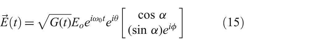
\vec{E} (t) = \sqrt{G (t)} E_{o} e^{i ω_{0} t} e^{i θ} [\begin{matrix} \cos α \\ (\sin α) e^{i ϕ} \end{matrix}]

(15)

where a time-dependent power envelope $\sqrt{G (t)}$ is represented as a composite shape using the sum of three Gaussian functions each with a scalar, mean, and standard deviation over a specified pulse duration $Δ t$ . The pulse’s electric field amplitude $E_{0}$ is used as a multiplier to the shape to determine the amount of energy in the pulse. The central frequency $ω_{0}$ captures the pulse’s oscillation, while the global phase θ is used to determine an offset for interference calculations in the simulation framework. The pulse’s encoded polarization state is captured by the orientation angle α with respect to the x axis, while ellipticity is used to represent the relative phase delay ϕ for phase-based QKD encoding. Method calls are used to calculate pulse wavelength, peak power, MPN, and pulse energy from the pulse’s shape, amplitude, duration, and central frequency. This wave representation allows for efficient calculation of optical effects such as propagation, dispersion, attenuation, or interference by individual optical components.

Figure 4.

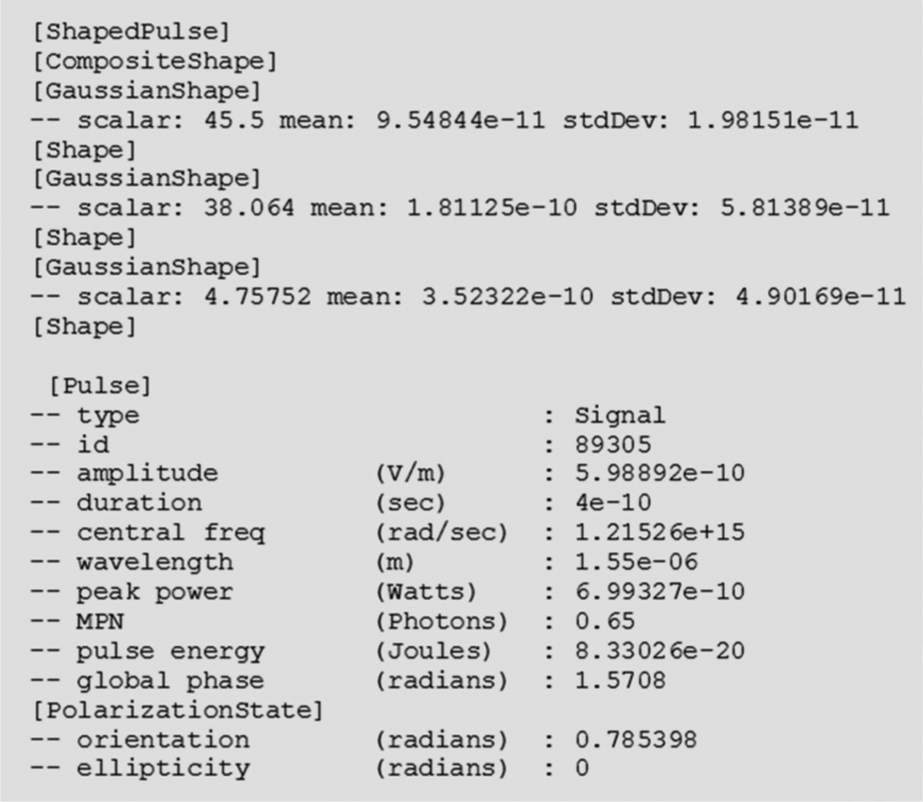
Modeled optical pulse.

4.2. Component verification

Component verification was conducted for each of the modeled optical components (laser, polarization modulator, electronic variable optical attenuator, fixed optical attenuator, fiber channel, beamsplitter, polarizing beamsplitter, half wave plate, and other components not shown such as a bandpass filter, circulator, in-line polarizer, isolator, optical switch 1×2, polarization controller, and wave division multiplexer). We used analytical means to verify the component models according to theory combined with commercial specifications and measured data. Specifically, the modeled components were implemented in C++ and verified using Python. This testing approach is intended to provide a flexible capability for verification of optical components, where new or modified components can be easily added and tested.

Testing focused on verifying the primary behaviors of each modeled component by ensuring the expected pulse transformations occur correctly. This was accomplished by comparing each model’s results (i.e., the pulse’s shape, amplitude, duration, central frequency, global phase, orientation, and ellipticity) to independent reference calculations over their specified operational ranges. An example of this testing methodology is provided in Table 5, where five input pulses with varying orientations (0, $π / 8, π / 4, 3 π / 8$ , and $π / 2$ ) and a fixed MPN of 0.6500 are shown propagating through a polarizing beamsplitter (note this example is greatly simplified for the reader, actual tests included 10,000s of points). The polarizing beamsplitter is modeled with one input and two outputs configured to split the input pulse according to the transmitted polarization (i.e., an orientation of 0) and the reflected polarization (i.e., an orientation of $π / 2$ ). The device is designed to project the input pulse’s energy (i.e., MPN) onto the transmitted and reflected polarization states. For example, since the first pulse’s orientation is 0, the entirety of the pulse’s energy will be transmitted and none will be reflected as demonstrated by both the modeled and truth data output results. Likewise, when considering the fourth pulse, we expect a small portion (~15%) of the energy to be observed on the transmitted port and a large amount (~85%) on the reflected port. This type of testing regime was automated in the framework and repeated thousands of times across pertinent operational and configuration parameters for each optical device in the component library. These components are modeled with ideal behaviors that result in perfect agreement to the expected values. Non-ideal behaviors caused by device imperfections or misuse can also be simulated. For example, each component is modeled with three operational states: normal, degraded, and damaged, where the device can enter the degraded or damaged state due to overheating or overpowering with optical light, which can negatively impact the devices’ behavior(s).

Table 5.

Polarizing beamsplitter verification.

Input pulses			Modeled output pulses		Truth data output pulses
Number	MPN	Orientation	Transmitted MPN(Orientation = 0)	Reflected MPN(Orientation = $π / 2$ )	Transmitted MPN(Orientation = 0)	Reflected MPN(Orientation = $π / 2$ )
1	0.6500	0	0.6500	0.0000	0.6500	0.0000
2	0.6500	$π / 8$	0.5548	0.0952	0.5548	0.0952
3	0.6500	$π / 4$	0.3250	0.3250	0.3250	0.3250
4	0.6500	$3 π / 8$	0.0952	0.5548	0.0952	0.5548
5	0.6500	$π / 2$	0.0000	0.6500	0.0000	0.6500

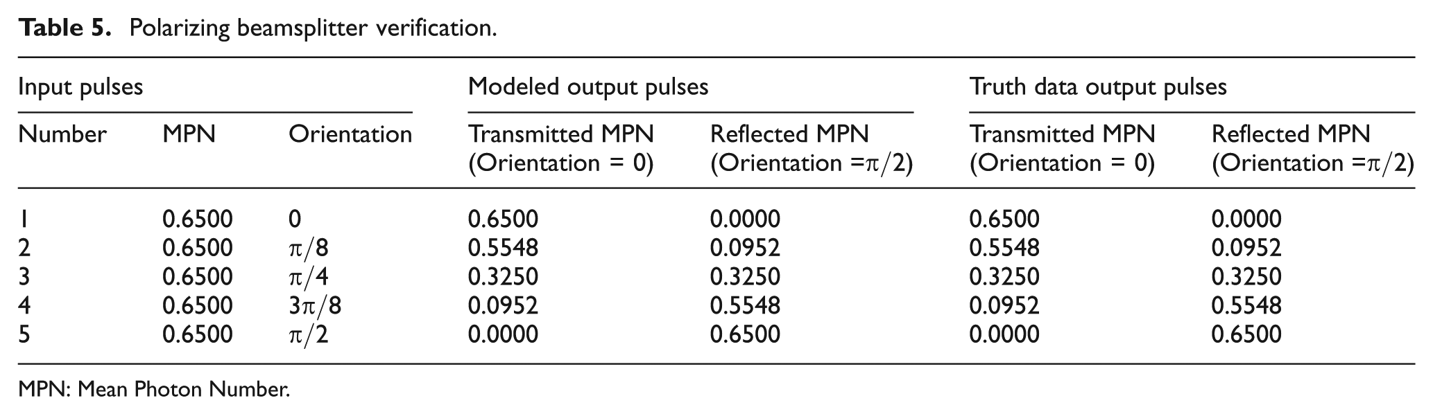
MPN: Mean Photon Number.

4.3. Sub-system verification

Sub-system verification was conducted using the experimental configuration as reported in Chen et al., where the USTC-Xinglin QKD architecture employed a signal MPN of 0.65, a decoy MPN of 0.08, a measured channel loss of 4.5 dB, and a reported 3.5 dB loss in Bob.⁵¹ From the sub-system perspective there are three points of interest in the communication system: (a) Alice’s output; (b) Bob’s input; and (c) Bob’s SPDs. For each point, we used analytical means to verify the state of the optical pulse for the expected and modeled MPNs and polarization orientation. Table 6 depicts the sub-system verification results where two pulses, a signal and a decoy, are tracked throughout the simulation using its unique identifier.

Table 6.

Sub-system verification of pulse MPN and orientation.

Alice’s output				Bob’s input			Bob’s SPDs
Pulse ID	Type	MPN	Orientation	Channel loss	MPN	Orientation	Bob’s loss	MPN	Orientation
4396	Signal	0.650000	$π / 2$	4.5 db	0.179025	$π / 2$	3.5 dB	0.079967	$π / 2$
Expectedresult		0.650000	$π / 2$		0.179025	$π / 2$		0.079967	$π / 2$
34811	Decoy	0.080000	$π / 4$		0.022034	$π / 4$		0.009842	$π / 4$
Expected result		0.080000	$π / 4$		0.022034	$π / 4$		0.009842	$π / 4$

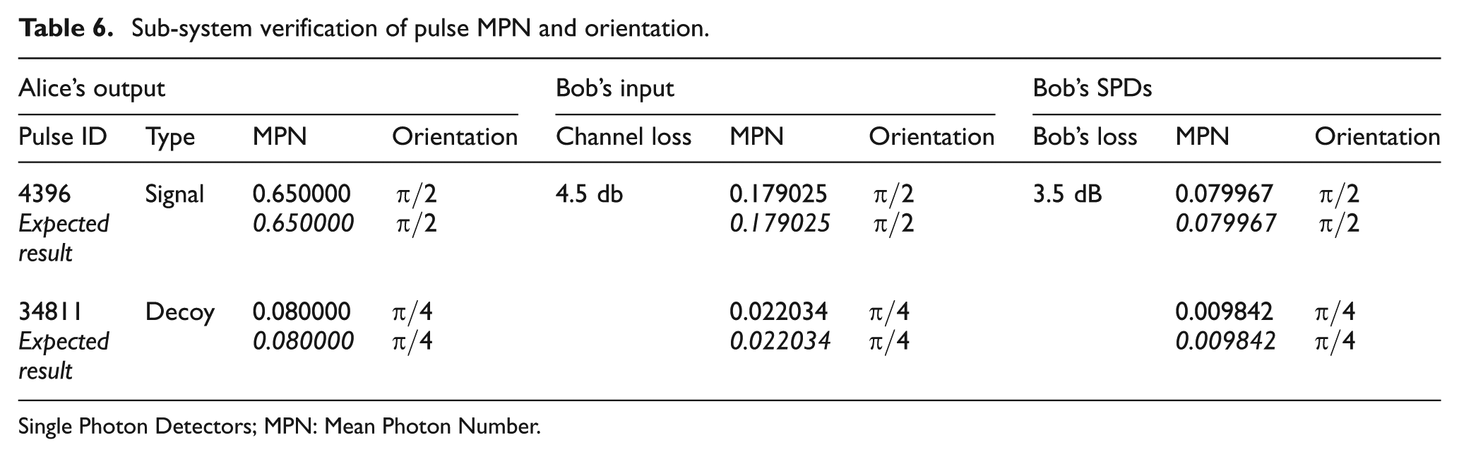
Single Photon Detectors; MPN: Mean Photon Number.

Each pulses’ MPN was verified against analytical calculations proving the modeled components were integrated properly. Verifying these three points ensures our optical pulse is propagating correctly through the end-to-end quantum path in preparation for system-level validation. Finally, we verified the expected signal, decoy, and vacuum occurrence percentages at Alice’s output with an average of 74.99978%, 12.50350%, and 12.49672% for 120 trials of 28,000 detections.

4.4. System validation

We conducted validation against similar systems, providing valid ranges of operation for our decoy state QKD model. Specifically, we chose five systems representative of a short operational distance (i.e., 20 km)^32,51–54 and three of a longer distance (i.e., 60 km).^33,55,56 The details reported in these articles, including architectural design, configuration parameters, and performance results lend themselves to a thorough validation effort. Operational parameters and results from each of the eight systems are presented in Table 7, along with results from representative models. Each of the simulated models include system implementations details such as signal and decoy MPNs, occurrence percentages, channel losses, receiver losses, detector efficiency, and detector dark count. The simulation results are reported for 60 trials of 50,000 detections each for a total of nearly 100,000,000 pulses sent per experimental treatment to provide statistically significant comparisons to the reported signal and decoy state gains and QBERs.

Table 7.

Validation results.

QKD system	Distance (km)	MPN μ / ν	Percent μ / ν	Channel loss (db)	Receiver loss (dB)	Detector efficiency (%)	Signal gain Q_μ ^**	Decoy gain Q_ν ^**	Signal QBER E_μ	Decoy QBER E_ν	R_secure ***
Chen et al. (Chen, et al., 2009)	20	0.60 / 0.08	75.0 / 12.5	5.6	3.5	10	6.36E-3	8.61E-4	1.44E-2	7.80E-2	4.10E-4
Model results							6.14E-3	9.61E-4	1.21E-2	6.57E-2	6.68E-4
Dixon et al. (Dixon, Yuan, Dynes, Sharpe, & Shield, 2008)	20	0.55 / 0.10	80 / 16	4.012	4.2^*	10	8.680E-3	1.970E-3	2.530E-2	Not reported	9.909E-4^*
Model results							6.775E-3	1.681E-3	1.44E-2	1.68E-2	11.755E-4
Yuan et al. (Yuan, Sharpe, & Shields, 2007)	25	0.425 / 0.204	75 / 25	4.7	2.5	10^*	8.500E-3	4.000E-3	1.720E-2	2.74E-2	8.806E-4^*
Model results							6.392E-3	3.275E-3	1.44E-2	2.44E-2	12.013E-4
Dynes et al. (Dynes, Yuan, Sharpe, & Shields, 2007)	20	0.55 0.098	93.0 / 6.2	4.0^*	2.5	10	1.270E-2	2.340E-3	1.80E-2	6.200E-2	1.464E-3^*
Model results							9.296E-3	1.968E-3	1.24E-2	3.96E-2	2.093E-3
Zhao et al. (Zhao, Qi, Ma, Lo, & Qian, 2006)	15	0.8 / 0.12	90 / 10	3.15	6.4^*	10^*	8.757E-3	1.360E-3	9.536E-3	2.689E-2	3.588E-4
Model results							6.039E-3	1.045E-3	9.219E-3	3.890E-2	5.586E-4

Dixon et al. (Dixon, Yuan, Dynes, Sharpe, & Shields, 2010)	50	0.5 / 0.1	98.83 / 0.78	10	3.5	16.5	4.00E-3	1.00E-3	3.85E-2	1.30E-2	2.590E-04
Model results							2.39E-3	9.76E-4	9.61E-2	2.33E-1	4.536E-4
Zhao et al. (Zhao, Qi, Ma, Lo, & Qian, 2006)	60	0.55 / 0.152	63.5 / 20.3	12^*	3.0^*	10	1.81E-3	5.47E-4	3.05E-2	7.78E-2	1.018E-4
Model results							1.50E-3	4.93E-4	2.51E-2	7.86E-2	1.6996E-4
Peng et al. (Peng, et al., 2007)	75	0.6 / 0.2	50 / 40	15.15	7.775	6.5	2.08E-4	7.53E-5	3.23E-2	9.04E-2	1.1430E-5
Model results							2.70E-4	1.04E-4	2.91E-2	7.30E-2	1.8560E-5

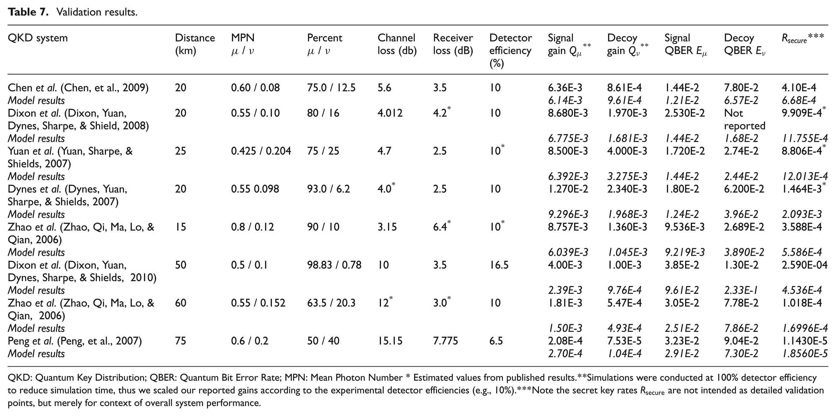
QKD: Quantum Key Distribution; QBER: Quantum Bit Error Rate; MPN: Mean Photon Number * Estimated values from published results. ** Simulations were conducted at 100% detector efficiency to reduce simulation time, thus we scaled our reported gains according to the experimental detector efficiencies (e.g., 10%). *** Note the secret key rates R_secure are not intended as detailed validation points, but merely for context of overall system performance.

Each QKD system is entirely unique, where the reported results are dependent upon dozens of operational and implementation details including calibration of the optical channel, programming of device controllers, various device imperfections, and the changing operational environment. Therefore, in these validation activities, we do not attempt to precisely match the reported performance but rather we attempt to replicate their results with a reasonable level of accuracy to justify the use of our model. That is, we prove sufficient accuracy for the intended purpose of studying the decoy state protocol. Specifically, by modeling the operational configuration parameters of Table 7, as well as the reported dark count and after pulse probabilities, we achieve simulation results within the same order of magnitude as the reported experimental system gains $Q_{μ}$ , $Q_{ν}$ , and QBERs $E_{μ}$ , $E_{ν}$ with $≲ 25 %$ relative error. Additionally, we list the reported and modeled secret key rates Rsecure; however, these results depend on a number of information theory techniques such as entropy estimation and privacy amplification, of which the implementation details are typically not publically disclosed. In our model, we estimate the entropy loss as 2^* QBER and randomly remove the appropriate percentage of bits from the final key. Thus, the secret key rates are provided merely as a cursory comparison of our model’s final secure key rate to the systems of interest.

By modeling and simulating architectural details such as reported propagation distances, losses, MPNs, occurrence percentages, and detector efficiencies we have ensured our model is consistent with decoy state enabled QKD systems for operational distances of 20 km and 60 km. Our verification activities ensured the model was built correctly, while our validation activities provide objective evidence that we built the correct model. These V&V activities provide analytical and experimental evidences for the accurate modeling of decoy state QKD systems to support further research and performance analysis.

5. Considerations for the decoy state protocol security condition

While the V&V activities described herein were primarily focused on ensuring the correctness of modeled behaviors, they also provide insight into practical considerations for implementing the decoy state protocol security condition which have not been explicitly addressed in other literature. In this section, we first introduce the security condition and then discuss practical implementation issues and initial findings from modeling, verifying, and validating these behaviors.

5.1 The decoy state protocol security condition

Recall, the decoy state protocol security condition was introduced to detect differences between the decoy and signal state statistics caused by the PNS attack, where the general premise is simply that channel losses and induced errors should remain constant over a given quantum channel. Formally, the decoy state protocol security condition is described as^28,30

Y_{n} = Y_{n}^{signal} = Y_{n}^{decoy}

(16)

e_{n} = e_{n}^{signal} = e_{n}^{decoy}

(17)

where the photon number dependent yield $Y_{n}$ is defined as the conditional probability that Bob detects an optical pulse given Alice sent an $n$ -photon. Similarly, the photon number dependent QBER $e_{n}$ is defined as the conditional probability an error occurred given Bob detects the $n$ -photon pulse from Alice.^28,30

The security condition asserts the yields $Y_{n}$ and QBERs $e_{n}$ for the signal and decoy states should always be the same (i.e., within prescribed tolerances) for each $n$ -photon pulse. This is because the quantum transmission efficiency and error rate are relatively fixed for a given QKD architecture. For example, when no interference is present $Y_{1}^{signal} = Y_{1}^{decoy}$ should always be true because the end-to-end transmission efficiency does not change; thus the likelihood of any pulse with one photon propagating from Alice to Bob is identical, regardless of its state. Likewise, the QBERs $e_{n}$ are based on device and alignment imperfections and should always be the same for each $n$ -photon pulse. Thus $Y_{n}$ and $e_{n}$ vary only with respect to the photon number per pulse $n = 1, 2, 3, \dots, n$ .

5.2 Implementing the decoy state security condition

In practical QKD implementations, the photon number dependent yields $Y_{n}^{signal}, Y_{n}^{decoy}$ and QBERs $e_{n}^{signal}, e_{n}^{decoy}$ are merely estimates of expected values because realized QKD system often use commercially available Avalanche Photodiode Detectors (APDs), which, cannot determine the specific number of photons received in each optical pulse. Therefore, Bob cannot precisely measure the $n$ -photon yields $Y_{n}$ or QBERs $e_{n}$ ; they must be estimated from the measured state gains $Q_{μ}, Q_{v,}$ and QBERs $E_{μ}, E_{v}$ . We will address the photon dependent yields $Y_{n}$ and then the QBERs $e_{n}$ .

5.3 Estimating photon number dependent yields

The photon number depended yield $Y_{n}$ is defined as^28,30

Y_{n} = Y_{0} + η_{n} - Y_{0} η_{n} ≅ Y_{0} + η_{n}

(18)

where $Y_{0}$ is the dark count described in Table 4, $η_{n}$ is the photon number dependent efficiency (see equation (19)), and the joint probability $Y_{0} η_{n}$ is typically disregarded because it is very small compared to $Y_{0}$ and $η_{n}$ . Treating each photon independently, the photon number dependent efficiency $η_{n}$ is based on the number of photons $n$ in each pulse and the end-to-end efficiency η (commonly expressed as the likelihood of successful propagation or in the negative sense as loss measured in dB)

η_{n} = 1 - {(1 - η)}^{n}

(19)

where

η = η_{QuantumChannel} η_{Bob} η_{detector} .

(20)

The overall quantum communication system efficiency η is the product of the quantum channel efficiency $η_{QuantumChannel}$ , the receiver’s efficiency $η_{Bob}$ , and the efficiency of the Bob’s detector $η_{detector}$ . The quantum channel efficiency is often approximated according to its length as $η_{QuantumChannel} = 10^{- 0.20 * ℓ ength / 10}$ or simply measured as a loss in dB. Bob’s efficiency $η_{Bob}$ is dependent on his internal design and typically measured as loss in dB. Bob’s detector efficiency $η_{detector}$ is device dependent and typically represented as a percentage. When studying the decoy state protocol, the protocol efficiency $η_{protocol}$ must also be considered, thus

η = η_{QuantumChannel} η_{Bob} η_{detector} η_{protocol} .

(21)

The protocol efficiency $η_{protocol}$ accounts for the signal state occurrence percentage (i.e., < 100%). For example, in the Chen et al. QKD system, only 75% of the transmitted pulses contribute to overall signal gain, while the decoy state account for 12.5%, and vacuums account for the remaining 12.5%. These operational parameters are part of an overall system trade space which directly impacts system performance.

The systems quantum efficiency η can be measured using device specific calibration activities or calculated as described in equation (21). As described by Lo et al. the quantum efficiency must be known in order to execute the decoy state security condition to detect PNS attacks [28], where the efficiency η along with the measured gains $Q_{μ}$ and $Q_{ν}$ is used to calculate the yields $Y_{n}^{signal}, Y_{n}^{decoy}$ . In this manner, Alice and Bob can reasonably bound the expected signal and decoy state yields $Y_{n}$ . For example, during normal operation, the yields $Y_{n}^{signal}$ are estimated using the polynomial relationship described in^28,30

Q_{μ} = Y_{0} e^{- μ} + Y_{1} e^{- μ} μ + Y_{2} \frac{e^{- μ} μ^{2}}{2} + \dots + Y_{n} \frac{e^{- μ} μ^{n}}{n!}

(22)

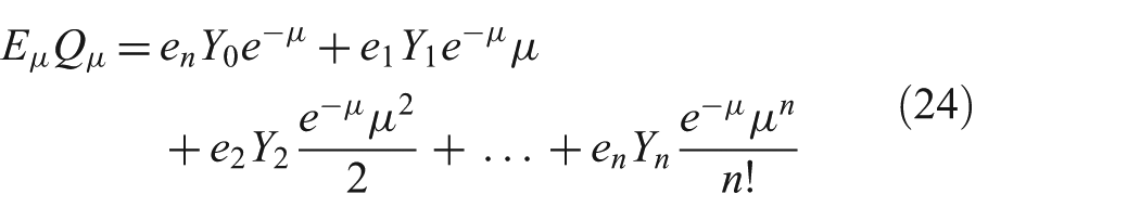
where μ is the signal state MPN and $n \leq 5$ typically provides sufficient accuracy to assess eavesdropping. Likewise, the the decoy state gain $Q_{ν}$ is used to estimate the decoy state yields $Y_{n}^{decoy}$ . The decoy and signal state photon statistics can then be compared to assess whether unauthorized photon specific interference exists on the quantum channel where $Y_{n}^{signal} \neq Y_{n}^{decoy}$ implies photon number specific interference on the quantum channel.

5.4 Estimating photon number dependent QBERs

The photon number dependent QBER $e_{n}$ is defined as^28,30

e_{n} = \frac{Y_{0} e_{0} + η_{n} e_{detection}}{Y_{n}}

(23)

where $Y_{0}$ is the dark count described in Table 4, $e_{0}$ is the likelihood of an error during a vacuum state (i.e., ½ since the erroneous detection results in either a 0 or 1), $η_{n}$ is the photon number dependent efficiency, and $e_{detection}$ is the probability a photon was detected at the wrong detector (i.e., due to device imperfections or misalignment, typically ∼1%²⁶). 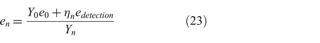The $n$ -photon QBER $e_{n}$ is estimated from the measured gain and QBER, where the relationship between the signal state QBER $E_{μ}$ , and the gain $Q_{μ}$ defined as

\begin{array}{l} E_{μ} Q_{μ} = e_{n} Y_{0} e^{- μ} + e_{1} Y_{1} e^{- μ} μ + \\ e_{2} Y_{2} \frac{e^{- μ} μ^{2}}{2} + \dots + e_{n} Y_{n} \frac{e^{- μ} μ^{n}}{n!} \end{array}

(24)

The end-to-end efficiency η, the decoy state gain $Q_{ν}$ , and the decoy state QBER $E_{ν}$ can be used to estimate the photon number dependent decoy state QBER $e_{n}^{decoy}$ . The photon number dependent QBERs can then be compared to assess whether unauthorized photon specific interference exists on the quantum channel where $e_{n}^{signal} \neq e_{n}^{decoy}$ implies eavesdropping on the quantum channel.

5.5 Security condition example

Assuming an eavesdropper is not going to knowingly introduce errors, Eve’s detectability is primarily dependent upon the system’s ability to detect changes in the yields $Y_{n}$ ; therefore, we examine the estimated photon number dependent yields $Y_{n}$ , $Y_{n}^{signal}$ , and $Y_{n}^{decoy}$ as shown in Table 8. For each row, the $n$ -photon yield is calculated using the derived signal or decoy state efficiencies based on the Chen et al. USTC-Xinglin QKD system. In the first column, the yields $Y_{n}$ are calculated from the reported channel efficiency of 5.6 dB, Bob’s efficiency of 3.5 dB, detector efficiency of 10%, and protocol efficiency of 75%, where the total efficiency $η = 0.009541$ per equation (21). Next, the yields $Y_{n}^{signal}$ and $Y_{n}^{decoy}$ are calculated from the measured gains $Q_{μ}$ and $Q_{ν}$ , respectively using equation (22).

Table 8.

Example photon dependent yields.

Photon number	Yield $Y_{n}$	Signal yield $Y_{n}^{signal}$	Decoy yield $Y_{n}^{decoy}$
n = 1	0.009641	0.009761	0.009616
n = 2	0.019090	0.019329	0.019042
n = 3	0.028450	0.028804	0.028378
n = 4	0.037720	0.038188	0.037625
n = 5	0.046902	0.047481	0.046784

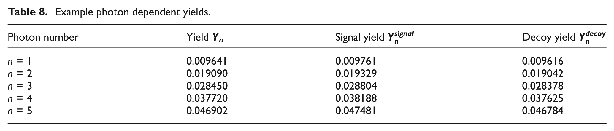
As the reader can ascertain, the photon specific yields are similar but not the same in all cases. We now turn our attention to understanding these differences in the form of implementation considerations and allowable tolerances.

5.6 Security condition considerations

In order to effectively implement the decoy state protocol, there are a number of design, implementation, and operational considerations to consider, including signal and decoy MPNs, occurrence percentages, propagation distances, total losses, desired detection sensitivity, the number of signal, decoy, and vacuum detections, and their resultant confidence intervals, amongst others. Therefore, when attempting to execute the decoy state protocol security condition, there needs to be additional consideration for implementation non-idealities and operational tolerances such that the security condition becomes

Y_{n}^{signal} = Y_{n}^{decoy} \pm Δ

(25)

e_{n}^{signal} = e_{n}^{decoy} \pm Δ

(26)

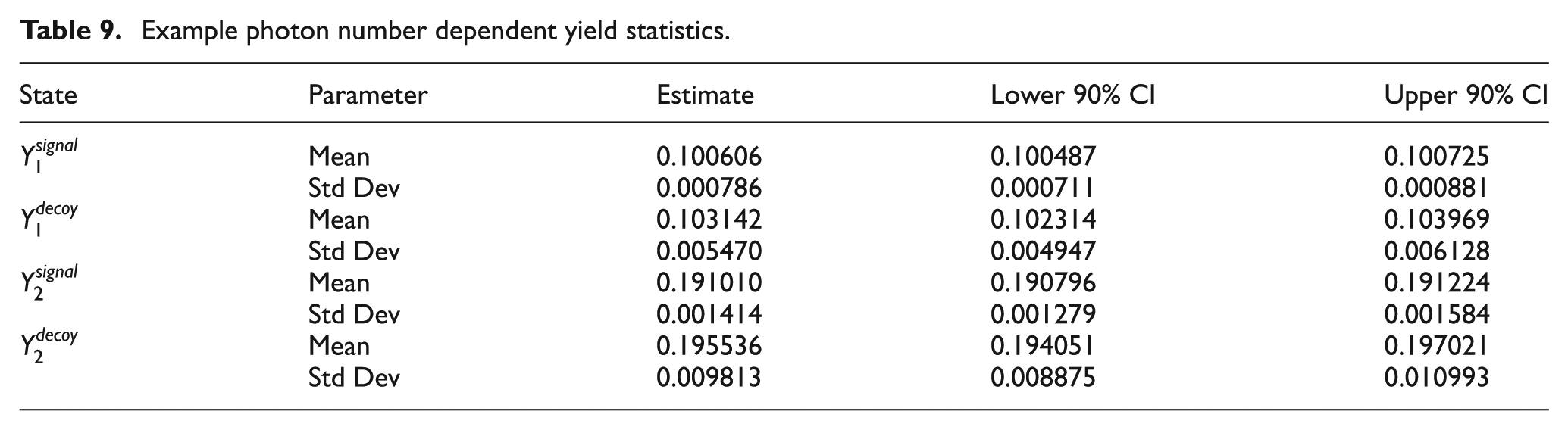
where Δ describes the expected variation in system operation. For example, in 120 trials designed to collect qubits for error reconciliation blocks of 10,000 bits (i.e., ~28,000 detections when accounting for 75% signal state and 50% sifting), we observed variations in both the signal and decoy photon dependent yields as depicted in Figure 5 and reported in Table 9. This is primarily due to expected probabilistic behavior in the number of detections and total number of pulses sent in each trial. 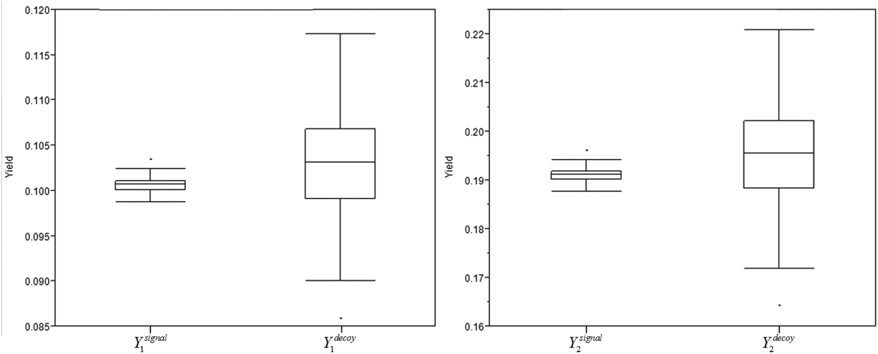In both $Y_{1}$ and $Y_{2}$ , the signal state has tighter bounds than the decoy state because of its higher MPN and occurrence percentage.

Figure 5.

Example photon dependent yields for n = 1 (left) and n = 2 (right). Note scales are different.

Table 9.

Example photon number dependent yield statistics.

State	Parameter	Estimate	Lower 90% CI	Upper 90% CI
$Y_{1}^{signal}$	Mean	0.100606	0.100487	0.100725
$Y_{1}^{signal}$	Std Dev	0.000786	0.000711	0.000881
$Y_{1}^{decoy}$	Mean	0.103142	0.102314	0.103969
$Y_{1}^{decoy}$	Std Dev	0.005470	0.004947	0.006128
$Y_{2}^{signal}$	Mean	0.191010	0.190796	0.191224
$Y_{2}^{signal}$	Std Dev	0.001414	0.001279	0.001584
$Y_{2}^{decoy}$	Mean	0.195536	0.194051	0.197021
$Y_{2}^{decoy}$	Std Dev	0.009813	0.008875	0.010993

5.7 Implementation considerations

When considering implementation of the decoy state protocol, one should first consider that decoy states have been primarily used to increase secret key rates and not necessarily for the ability to detect PNS attacks; there has been little formal consideration of the effectiveness of the decoy state security condition in detecting eavesdroppers in the published literature. Therefore, we provide an enumerated list of practical implementation considerations and operational configuration issues which merit further examination:

Accuracy in signal and decoy state MPNs

Difference between signal and decoy state MPNs

Ratio of signal, decoy, and vacuum occurrence percentages

The impact of losses through the end-to-end quantum path

Induced errors between Alice and Bob, including reference alignment, timing synchronization, and bias in photon detection

Statistical confidence of decoy state security related parameters

Monitoring of alternate decoy state security measurable parameters such as the ratio between $Q_{μ}$ and $Q_{ν}$ as suggested in Yuan et al.⁵⁴ or η for the signal and decoy state

Trade space definition between system performance (i.e., secret key rate) and security posture (i.e., detectability of an eavesdropper)

Lastly, we suggest conventional security practices such as operating from a known secure state and continuous monitoring be integrated into QKD system design and operation. For example, an independent characterization of channel losses, Bob’s internal losses, detector efficiency, and protocol efficiency can be used as an additional security check for validating and ensuring expected yields $Y_{n}$ are close to expected operational yields $Y_{n}^{signal}$ , $Y_{n}^{decoy}$ . These types of checks could easily be incorporated during initialization and operation of QKD systems, or during periodic security checks or re-calibration activities.

6. Conclusions

This paper provides a detailed discussion of a modeled decoy state enabled QKD system. We demonstrated component and sub-system verification activities, as well as, system-level validation proving the model’s correctness and applicability for further performance and security analysis. Lastly, based on our work modeling of a decoy state enabled QKD system, we bring attention to practical considerations for executing the decoy state protocol security condition, including design considerations and allowable tolerances.

Future work includes studying the decoy state enabled QKD system’s ability to detect photon number specific attacks, accomplishing sensitivity analysis of operational parameters, conducting system-level performance characterization with respect to decoy state protocol security condition, and defining the security-performance trade space.

Footnotes

Disclaimer

The views expressed in this paper are those of the authors and do not reflect the official policy or position of the United States Air Force, the Department of Defense, or the U.S. Government.

Declaration of Conflicting Interest

The authors declare that there is no conflict of interest.

Funding

This work was supported by the Laboratory for Telecommunication Sciences [grant number 5743400-304-6448].

Notes

Author biographies

Logan O. Mailloux, CISSP, CSEP (BS 2002, MS 2008) is a commissioned officer in the United States Air Force and a PhD candidate at the Air Force Institute of Technology (AFIT), Wright-Patterson AFB, Ohio, USA. His research interests include system security engineering, complex information communication and technology implementations, and quantum key distribution systems. He is a member of Tau Beta Pi, Eta Kappa Nu, INCOSE, the ACM, and IEEE. He can be contacted at logan.mailloux@afit.edu.

Ryan D. Engle, (BS 2007, MS 2015) is a commissioned officer in the United States Air Force and a PhD student at the Air Force Institute of Technology (AFIT), Wright-Patterson AFB, Ohio, USA. His research interests include software engineering, computer engineering, model-based systems engineering, modeling and simulation, and quantum key distribution systems. He is a member of the ACM and IEEE. He can be contacted via email at ryan.engle@afit.edu.

Michael R. Grimaila, PhD, CISM, CISSP (BS 1993, MS 1995, PhD 1999) is Professor and Head of the Systems Engineering department and member of the Center for Cyberspace Research (CCR) at the Air Force Institute of Technology (AFIT), Wright-Patterson AFB, Ohio, USA. He is a member of Tau Beta Pi, Eta Kappa Nu, the ACM, a Senior Member of the IEEE, and a Fellow of the ISSA. His research interests include computer engineering, mission assurance, quantum communications and cryptography, data analytics, network management and security, and systems engineering. He can be contacted via email at Michael.Grimaila@afit.edu.

Douglas D. Hodson, PhD (BS 1985, MS 1987, MBA 1998, PhD 2009) is an Assistant Professor of Computer Engineering at the AFIT, Wright-Patterson AFB, Ohio, USA. His research interests include computer engineering, software engineering, real-time distributed simulation, and quantum communications. He is also a DAGSI scholar and a member of Tau Beta Pi.

John M. Colombi, PhD (BS 1986, MS 1992, PhD 1996) is an Associate Professor of Systems Engineering at the Air Force Institute of Technology (AFIT), Wright-Patterson AFB, Ohio, USA. Before joining the faculty, Dr Colombi had 21 years of military experience, where he led systems engineering for the E-3 aircraft, managed C2ISR portfolio integration, developed and tested biometrics and information security, and researched secure tactical networking at the Air Force Research Laboratory. His research interests include systems and enterprise architecture, complex adaptive systems, acquisition process modeling and human systems integration. He is a member of the IEEE and INCOSE.

Colin V. McLaughlin, PhD (BA 2003, PhD 2010) is a Research Physicist at the United States Naval Research Laboratory, Washington, D.C., USA. He specializes in photonic communication devices and systems.

References

Mailloux

Grimaila

Hodson

. Performance evaluations of quantum key distribution system architectures. IEEE Secur Privacy 2015; 13(1): 30–40.

Morris

Grimaila

Hodson

. Using the discrete event system specification to model quantum key distribution system components. J Defense Modeling Simulat 2014: 1548512914554404.

Mailloux

. A modeling framework for studying quantum key distribution system implementation non-idealities. IEEE Access 2015: 110–130.

Gisin

Ribordy

Tittel

. Quantum cryptography. Rev Modern Phys 2002; 74(1): 145–195.

Scarani

Bechmann-Pasquinucci

Cerf

. The security of practical quantum key distribution. Rev Modern Phys 2009; 81(3): 1301–1350.

Loepp

Wooters

. Protecting information. New York: Cambridge University Press, 2006.

Nielsen

Chuang

. Quantum computation and quantum information. Cambridge University Press, 2010.

Office of Naval Research. Quantum information sciences program. U.S. Navy. n.d. http://www.onr.navy.mil/en/Science-Technology/Departments/Code-31/All-Programs/311-Mathematics-Computers-Research/Quantum-Information-Science.aspx (accessed October 23, 2014).

Department of the Army. U.S. Army Research Laboratory (ARL) Center for Distributed Quantum Information (CDQI). n.d. https://www.fbo.gov/index?s=opportunity&mode=form&tab=core&id=0ae2481dfa71231c782f6e03ace76195 (accessed October 23, 2014).

10.

U. S. Air Force Scientific Advisory Board. Utility of Quantum Systems for the Air Force. n.d.http://www.sab.af.mil/library/factsheets/factsheet.asp?id=21756 (accessed October 23 2014).

11.

ID Quantique SA. Main page. 2014. www.idquantique.com (accessed September 30 2014).

12.

SeQureNet. 2014. www.sequrenet.com (accessed September 30 2014).

13.

Quintessence Labs. 2014. www.quintessencelabs.com (accessed September 30 2014).

14.

MagiQ Technologies. 2014. www.magiqtech.com (accessed September 30 2014).

15.

QuantumCTek 2014. http://www.quantum-info.com/en.php (accessed May 28 2015).

16.

Wiesner

. Conjugate coding. ACM Sigact News, 1983: 78–88.

17.

Bennett

Brassard

. Quantum cryptography: Public key distribution and coin tossing. In: Proceedings of IEEE international conference on computers, systems and signal processing, 1984.

18.

Gilbert

. Cipher printing telegraph systems for secret wire and radio telegraphic communications. Trans Am Inst Electr Engrs 1926; 45: 295–301.

19.

Shannon

. Communication theory of secrecy systems. Bell System Tech J 1949; 28: 656-715.

20.

Renato

Gisin

Kraus

. An information-theoretic security proof for QKD protocols. Phys Rev A (arXiv:quant-ph/0502064) 2005; 72(1).

21.

Gottesman

H-K

Lutkenhaus

. Security of quantum key distribution with imperfect devices. In: Proceedings of International symposium on information theory, 2004. ISIT 2004. IEEE, 2004, p. 136.

22.

Scarani

Kurtsiefer

. The black paper of quantum cryptography: real implementation problems. arXiv:0906.4547v2, 2009.

23.

Bennett

Bessette

Brassard

. Experimental quantum cryptography. J Cryptol 1992; 5(1): 3–28.

24.

Huttner

Imoto

Gisin

. Quantum cryptography with coherent states. Phys Rev A 1995; 51(3): 1863.

25.

Brassard

Lutkenhaus

Mor

. Limitations on practical quantum cryptography. Phys Rev Lett 2000; 85(6): 1330.

26.

Lütkenhaus

. Security against individual attacks for realistic quantum key distribution. Phys Rev A 2000; 61(5): 052304.

27.

Hwang

W-Y

. Quantum key distribution with high loss: Toward global secure communication. Phys Rev Lett 2003; 91(5): 057901.

28.

H-K

Chen

. Decoy state quantum key distribution. Phys Rev Lett 2005; 94(3): 230504.

29.

Wang

X-B

. Beating the photon-number-splitting attack in practical quantum cryptography. Phys Rev Lett 2005; 94(23): 230503.

30.

Zhao

. Practical decoy state for quantum key distribution. Phys Rev 2005; 72(1): 012326.

31.

Wang

X-B

. Decoy-state protocol for quantum cryptography with four different intensities of coherent light. Phys Rev A 2005; 72(1): 012322.

32.

Zhao

. Experimental quantum key distribution with decoy states. Phys Rev Lett 2006; 96(7): 070502.

33.

Zhao

. Simulation and implementation of decoy state quantum key distribution over 60km telecom fiber. In: IEEE international symposium on information theory, 2006, 2006. 2094–2098.

34.

Wang

X-B

Peng

C-Z

Pan

J-W

. Simple protocol for secure decoy-state quantum key distribution with a loosely controlled source. Appl Phys Lett 2007; 90(3): 031110.

35.

Wang

X-B

Yang

Peng

C-Z

. Decoy-state quantum key distribution with both source errors and statistical fluctuations. New J Phys 2009; 11(7): 075006.

36.

J-Z

Wang

X-B

. Reexamination of the decoy-state quantum key distribution with an unstable source. Phys Rev A 2010; 82(1): 012331.

37.

J-Z

Wang

X-B

. Secure quantum key distribution in an easy way. arXiv:1004.3730, 2010.

38.

Harrington

Ettinger

Hughes

. Enhancing practical security of quantum key distribution with a few decoy states. arXiv, 2005: quant-ph/0503002.

39.

Horikiri

Kobayashi

. Decoy state quantum key distribution with a photon number resolved heralded single photon source. Phys Rev A 2006; 73(3).

40.

Hayashi

. General theory for decoy-state quantum key distribution with an arbitrary number of intensities. New J Phys 2007; 9(8).

41.

Mauerer

Silberhorn

. Quantum key distribution with passive decoy state selection. Phys Rev A 2007; 75(5): 050305.

42.

Brassard

Salvail

. Secret-key reconciliation by public discussion. In: Advances in cryptology: EUROCRYPT’93, 1994, pp.410–423.

43.

Lydersen

. Superlinear threshold detectors in quantum cryptography. Phys Rev A 2011; 84(032320).

44.

Mailloux

Grimaila

Hodson

. Modeling continuous time optical pulses in a quantum key distribution discrete event simulation. In: International Conference on Security and Management SAM’14, 2014.

45.

Giancoli

. Physics for scientists and engineers. Prentice Hall, 1989.

46.

Miller

. Quantum mechanics for scientists and engineers. Cambridge University Press, 2008.

47.

Sorensen

Grimaila

. Discrete event simulation of the quantum channel within a quantum key distribution system. J Defense Modeling and Simul: Appl, Methodol, Technol 1548512915569743 (2015).

48.

Sargent

. Verification and validation of simulation models. In: Proceedings of the 2010 Winter simulation conference, 2010, pp.166–183.

49.

Smith

Murray-Smith

Hickman

Verification and validation issues in a generic model of electro-optic sensor systems. J Defense Modeling Simul 2007; 4(1): 17–27.

50.

Roza

Voogd

Sebalj

. The generic methodology for verification and validation to support acceptance of models, simulations and data. J Defense Modeling Simul 2012; 10(4): 347–365.

51.

Chen

T-Y

. ‘Field test of a practical secure communication network with decoy-state quantum cryptography.’Opt Express 2009; 17(8): 6540–6549.

52.

Dixon

Yuan

Dynes

. Gigahertz decoy quantum key distribution with 1 Mbit/s secure key rate. Opt Express 200816(23): 18790–18979.

53.

Dynes

Yuan

Sharpe

. Practical quantum key distribution over 60 hours at an optical fiber distance of 20km using weak and vacuum decoy pulses for enhanced security. Op Express 2007; 15(13): 8465–8471.

54.

Yuan

Sharpe

Shields

. Unconditionally secure one-way quantum key distribution using decoy pulses. Appl Phys Lett 2007; 90(1): 011118.

55.

Dixon

Yuan

Dynes

. Continuous operation of high bit rate quantum key distribution. Appl Phys Lett 2010; 96(16): 161102.

56.

Peng

C-Z

. ‘Experimental long-distance decoy-state quantum key distribution based on polarization encoding. Phys Rev Lett 2007; 98(1): 010505.