Optimizing network microsegmentation policy for cyber resilience

Abstract

This paper describes an approach for improving cyber resilience through the synthesis of optimal microsegmentation policy for a network. By leveraging microsegmentation security architecture, we can reason about fine-grained policy rules that enforce access for given combinations of source address, destination address, destination port, and protocol. Our approach determines microsegmentation policy rules that limit adversarial movement within a network according to assumed attack scenarios and mission availability needs. For this problem, we formulate a novel optimization objective function that balances cyberattack risks against accessibility to critical network resources. Given the application of a particular set of policy rules as a candidate optimal solution, this objective function estimates the adversary effort for carrying out a particular attack scenario, which it balances against the extent to which the solution restricts access to mission-critical services. We then apply artificial intelligence techniques (evolutionary programming) to learn microsegmentation policy rules that optimize this objective function.

Keywords

Security policy optimization attack graphs genetic algorithms

1. Introduction

In modern military doctrine, armed conflict involves “multiple layers of stand-off” in all operational domains, including cyberspace.¹ Effective layering of defenses in cyberspace requires addressing all phases of the cyberattack lifecycle. Given increasingly complex networked systems and advanced cyber threats, there is growing recognition of the need for cyber resilience, that is, the ability to continue to operate in spite of ongoing cyberattacks.^2–4 For optimizing cyber resilience, a key challenge is being able to assess various candidate security policies under given mission and threat circumstances.

Assessment of security policy must consider not only potential impact from adversarial activities, but also any restricted availability of mission-critical services due to security hardening. This is especially true inside network perimeters, since systems and services that can be exploited by adversaries already inside a network are likely to be more critical (vs outside facing ones) for mission operations. Given indications of likely adversarial avenues of approach (or indicators of actual compromise) and measures of mission criticality for allowed access to network resources, policy rules can be optimized to account for that information. This requires fine granularity in how such rules are expressed and enforced.

A way of accomplishing the kind of fine-grained control over access policy needed for optimal cyber resilience is through network microsegmentation.⁵ Microsegmentation is a granular approach for workload isolation and security. More traditional methods of network segmentation secure traffic in the north-south (outside vs inside) orientation. Microsegmentation provides greater control over east-west (lateral) traffic inside a network, for example, for limiting lateral movement by adversaries who have breached perimeter defenses. With implementation through virtualization technology, microsegmentation supports flexible and adaptive security policy in response to changing mission requirements and threat situations. Examples of such virtualization in modern weapon systems include the US Army’s Command Post Computing Environment (CPCE) software deployed on Tactical Server Infrastructure (TSI).⁶

This paper describes an approach for optimizing network microsegmentation policy for maximum resilience. Through microsegmentation security architecture for enforcement, we consider sets of fine-grained policy rules that allow access for given combinations of source address, destination address, destination port, and protocol. Our approach analyzes the efficacy of candidate policy solutions with respect to (1) minimizing the risks of a particular threat situation while (2) maximizing accessibility to critical network resources. We formulate this as a novel optimization problem that quantifies attacker reachability in terms of multi-step exploitation. Unlike previous approaches, for example, Noel and colleagues^7,8 that require all exploitable paths to be broken for a given threat situation, we compute the numbers of potential attack walks of given lengths, which allows for quantitative comparisons among candidate policies for resiliency tradeoff analysis.

The numbers of attack walks provide an estimate of adversary effort resulting from the application of a candidate policy. The optimization problem is then a joint maximization of adversary effort and mission availability. In this way, we relax the brittle binary cut-set blocking of previous approaches. Instead, we measure to what extent a candidate policy solution blocks shorter (least adversary effort) exploitation paths, to allow tunable tradeoffs between security and usability.

We then apply artificial intelligence (AI) techniques (evolutionary algorithms) to learn the optimal microsegmentation policy according to the optimization objective, as part of the MITRE Adaptive Resiliency Experimentation System (ARES). ARES employs off-the-shelf cybersecurity tools and custom AI-powered components for optimizing cyber resilience, including microsegmentation, authentication, policy generalization, redundancy, deception, and zero-trust architecture. This paper focuses on the optimization of microsegmentation policy (allowed source/destination address, destination port, and protocol) in ARES, enforced through Amazon Web Service (AWS) security groups (virtual host-based firewalls).

The next section describes our approach for optimizing microsegmentation policy. Section 3 formulates our optimization problem in terms of the tradeoff between maximizing adversary effort and maximizing access to mission-critical resources. Section 4 describes key experimental results for our approach. Section 5 then summarizes our approach.

2. Technical approach

Figure 1 shows a high-level overview of our approach. In Data Collection, various host and network sensors forward data to a central repository, where the data elements are correlated across the sensor types. In Model Building, correlated network data are ingested and mapped to a model representing the network environment and mission/threat situation. In Policy Optimization, a set of microsegmentation rules is synthesized that provide optimal resiliency for the network as defined by the optimization objectives (maximizing adversary effort and mission availability).

Figure 1.

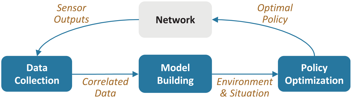
Overview of approach.

Policy optimization simulates potential multi-step lateral movement through the network according to a particular threat situation. The threat situation includes any presumed or detected adversarial presence in the network and identifies any mission-critical hosts that are to be prioritized for protection from the adversary. For a given candidate policy solution, the policy is applied to the network environment, and scored according to the optimization objective defined in section 3.

In general, the effects of microsegmentation rules on threats are combinatorial, so that the rules that comprise a candidate solution cannot be considered independently of one another. We apply evolutionary programming for searching the combinatorial space of rules to learn the optimal solution to this non-deterministic polynomial-time (NP)-hard optimization problem. In this way, we synthesize optimized policy that balances cyberattack risks and mission needs.

3. Problem formulation

A key result of ARES model building (Figure 1) is an inferred initial state of allowed connections, based on generalization of observed traffic via unsupervised learning (clustering). We treat this as a baseline policy for microsegmentation. This baseline policy is a set of rules, with each rule defined as an allowed combination of source address, destination address, destination port, and protocol. Our policy optimization then considers changes to the baseline policy, that is, a set of denied rules (with respect to the baseline set) that best meets an optimization fitness function.

In ARES, the baseline policy is represented as a graph, with host IP addresses as nodes and combinations of destination port and protocol as edges (a multigraph, since multiple destination port and protocol combinations are possible for a given source/destination IP pair). Nodes and edges also have various properties assigned to them, which encode information such as vulnerabilities that can be exploited by an adversary and mission criticality of network connections.

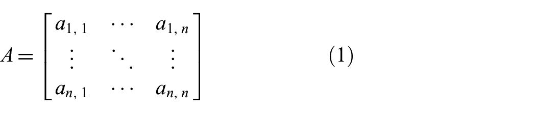
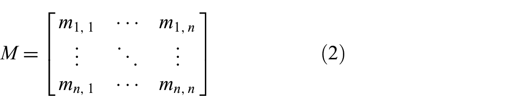
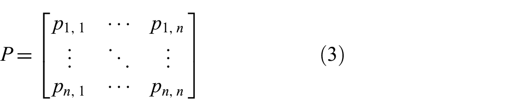
In our problem formulation, we define certain subgraphs of the baseline policy graph (casting multigraphs as simple graphs), which we apply for policy optimization. We represent these graphs as adjacency matrices, with computations needed for optimization expressed as matrix operations. This provides a convenient mathematical notation, as well as efficient implementation via established software and hardware such as sparse matrix processing and parallel processing with graphics processing units (GPUs).

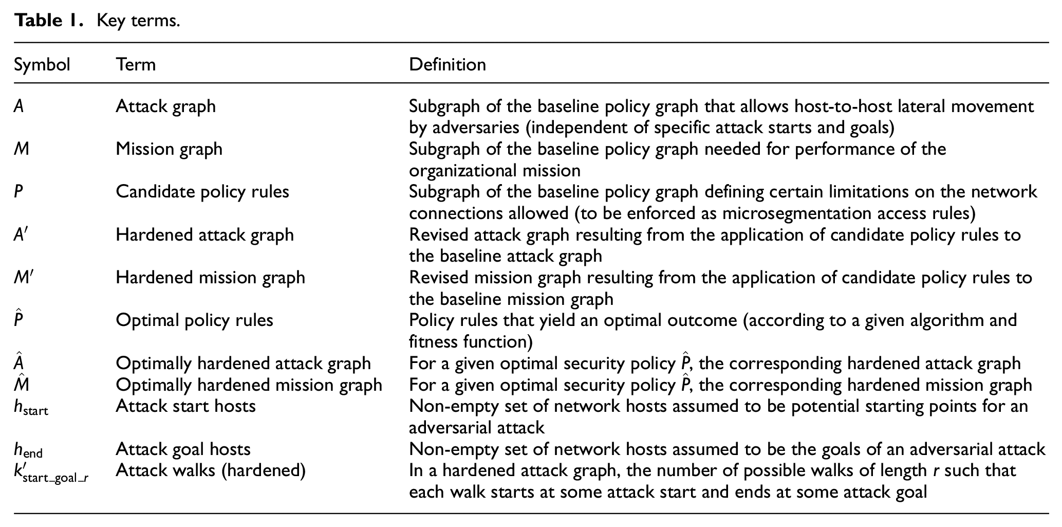
Table 1 lists key terms that are introduced in this section.

Table 1.

Key terms.

Symbol	Term	Definition
$A$	Attack graph	Subgraph of the baseline policy graph that allows host-to-host lateral movement by adversaries (independent of specific attack starts and goals)
$M$	Mission graph	Subgraph of the baseline policy graph needed for performance of the organizational mission
$P$	Candidate policy rules	Subgraph of the baseline policy graph defining certain limitations on the network connections allowed (to be enforced as microsegmentation access rules)
$A'$	Hardened attack graph	Revised attack graph resulting from the application of candidate policy rules to the baseline attack graph
$M'$	Hardened mission graph	Revised mission graph resulting from the application of candidate policy rules to the baseline mission graph
$\hat{P}$	Optimal policy rules	Policy rules that yield an optimal outcome (according to a given algorithm and fitness function)
$\hat{A}$	Optimally hardened attack graph	For a given optimal security policy $\hat{P}$ , the corresponding hardened attack graph
$\hat{M}$	Optimally hardened mission graph	For a given optimal security policy $\hat{P}$ , the corresponding hardened mission graph
$h_{start}$	Attack start hosts	Non-empty set of network hosts assumed to be potential starting points for an adversarial attack
$h_{end}$	Attack goal hosts	Non-empty set of network hosts assumed to be the goals of an adversarial attack
$k'_{start_goal_r}$	Attack walks (hardened)	In a hardened attack graph, the number of possible walks of length $r$ such that each walk starts at some attack start and ends at some attack goal

In section 3.1, we define foundational mathematical models that capture salient aspects of cyber resilience. In section 3.2, we start with ideal assumptions (constraints) about the problem space to define a restricted form of optimization. In section 3.3, we relax certain of those constraints to obtain a more realistic and meaningful problem formulation. In section 3.4, we relax a final constraint (mission-impact budget), yielding a multi-objective optimization problem that allows a Pareto-optimal tradeoff between security (thwarting an assumed attack scenario) and mission needs (minimizing impact from blocked services).

3.1. Mathematical foundations

For each optimization problem in this section, assume that we are given graphs that represent two kinds of host-to-host relationships: an attack graph $A$ and a mission graph $M$ . These represent a baseline state of allowed network connectivity before any candidate policy solutions are applied for resiliency optimization.

We express attack graph $A$ as an $n \times n$ binary adjacency matrix (for $n$ hosts), that is, the following:

A = [\begin{matrix} a_{1, 1} & \dots & a_{1, n} \\ ⋮ & ⋱ & ⋮ \\ a_{n, 1} & \dots & a_{n, n} \end{matrix}]

(1)

Here, binary element $a_{i, j}$ represents an attacker being able to reach (in terms of lateral network movement) directly (in one attack step) from host $i$ to host $j$ . In other words, direct connectivity is allowed from host $i$ to a vulnerable service on host $j$ if and only if $a_{i, j} = 1$ .

On the mission side, element $m_{i, j}$ of mission graph $M$ (expressed as an $n \times n$ adjacency matrix) encodes the need for host $i$ to reach host $j$ (directly) for the organizational mission, that is:

M = [\begin{matrix} m_{1, 1} & \dots & m_{1, n} \\ ⋮ & ⋱ & ⋮ \\ m_{n, 1} & \dots & m_{n, n} \end{matrix}]

(2)

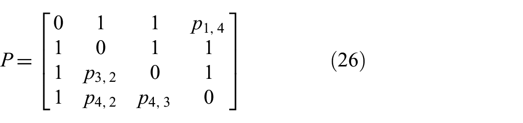
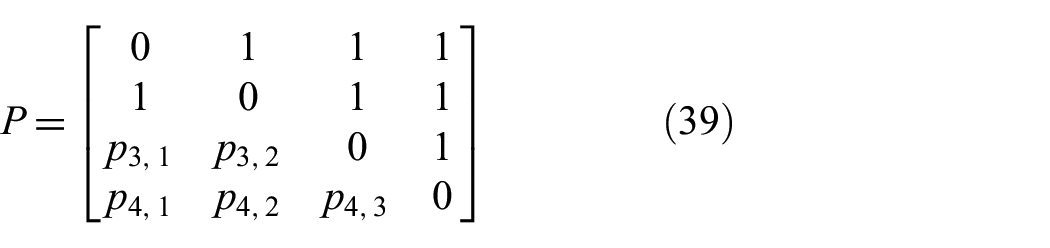
In some of our optimization problem formulations, the elements of $M$ are binary, with direct connectivity needed (and allowed) from host $i$ to a host $j$ if and only if $m_{i, j} = 1$ . In other problem formulations, we generalize $M$ to a weighted adjacency matrix, where positive integer $m_{i, j}$ quantifies the amount of mission need for host $i$ to be able to connect (directly) to host $j$ .

For a given instance of an optimization problem, a graph of candidate policy rules $P$ (expressed as an $n \times n$ adjacency matrix) encodes state transitions for allowed access from one host to another:

P = [\begin{matrix} p_{1, 1} & \dots & p_{1, n} \\ ⋮ & ⋱ & ⋮ \\ p_{n, 1} & \dots & p_{n, n} \end{matrix}]

(3)

That is, element $p_{i, j}$ represents a policy rule that either allows $(p_{i, j} = 1)$ or denies $(p_{i, j} = 0)$ access from host $i$ to host $j$ . For a given candidate policy rule graph $P$ , we apply the policy rules to the original attack graph $A$ . This forms a hardened attack graph $A'$ that results from the application of policy rules $P$ , that is:

A' = P ° A

(4)

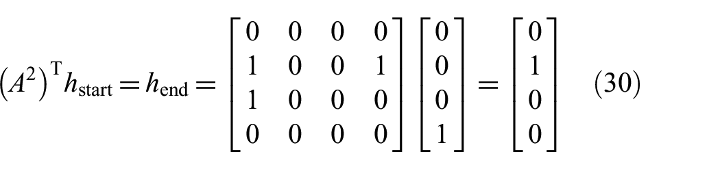
Here, the ° symbol denotes the Hadamard (elementwise) product,⁹ defined by $[A ° B]_{i, j} = [A]_{i, j} [B]_{i, j}$ , for all $1 \leq i, j < n$ . Similarly, we can apply policy rules $P$ to the original mission graph $M$ , yielding a hardened mission graph $M'$ :

M' = P ° M

(5)

The graphs $A'$ and $M'$ represent the application of policy rules (allows and denies between host pairs) that affect host-to-host reachability for an attacker and the mission (respectively). This allows an optimization algorithm to assess constraints and objectives for the optimization problem.

We can apply an optimal policy rules graph $\hat{P}$ to the original attack graph $A$ , yielding an optimally hardened attack graph $\hat{A}$ :

\hat{A} = \hat{P} ° A

(6)

Similarly, we can apply an optimal policy rules graph $\hat{P}$ to the original mission graph $M$ , yielding an optimally hardened mission graph $\hat{M}$ :

\hat{M} = \hat{P} ° M

(7)

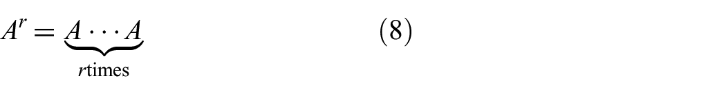
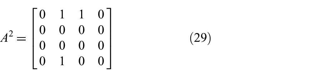
Leveraging the adjacency matrix representation for graphs, we can evaluate the existence of attack walks of a given length through matrix multiplication.^10,11 For a square $(n \times n)$ matrix $A$ and a positive integer $r$ , then $A^{r}$ is the product of $r$ instances of $A$ :

A^{r} = \underset{r times}{\underset{︸}{A \dots A}}

(8)

Here, matrix multiplication is in the usual sense,¹² that is, an element of $AA = A^{2}$ is:

{[A^{2}]}_{i, j} = \sum_{k} a_{i, k} \cdot a_{k, j}

(9)

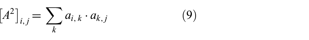
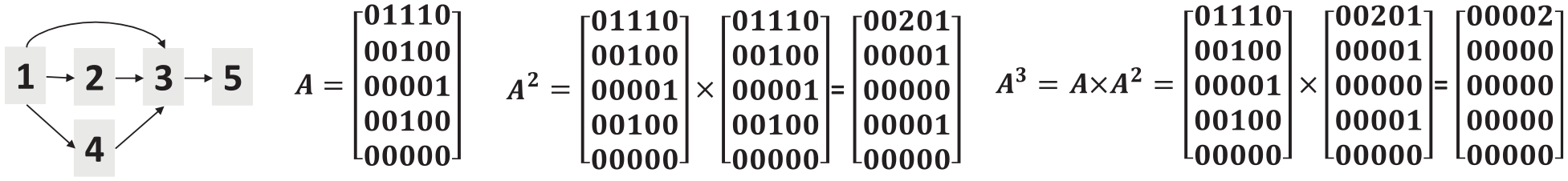
The matching of rows and columns in matrix multiplication corresponds to matching path steps of an attack graph, and the summation counts the numbers of matching steps. The elements of $A^{1} = A$ are the direct length-1 walks between host pairs. Then, each element of $A^{2}$ gives the number of length-2 walks between the corresponding pair (row and column) of attack graph vertices (hosts). Likewise, $A^{3}$ gives the numbers of length-3 walks, $A^{4}$ gives the numbers of length-4 walks, and so on. Figure 2 shows an example graph, its corresponding adjacency matrix $A$ , and the adjacency matrix raised to two and three powers (walks of length 2 and 3, respectively).

Figure 2.

Graph adjacency matrix and its powers.

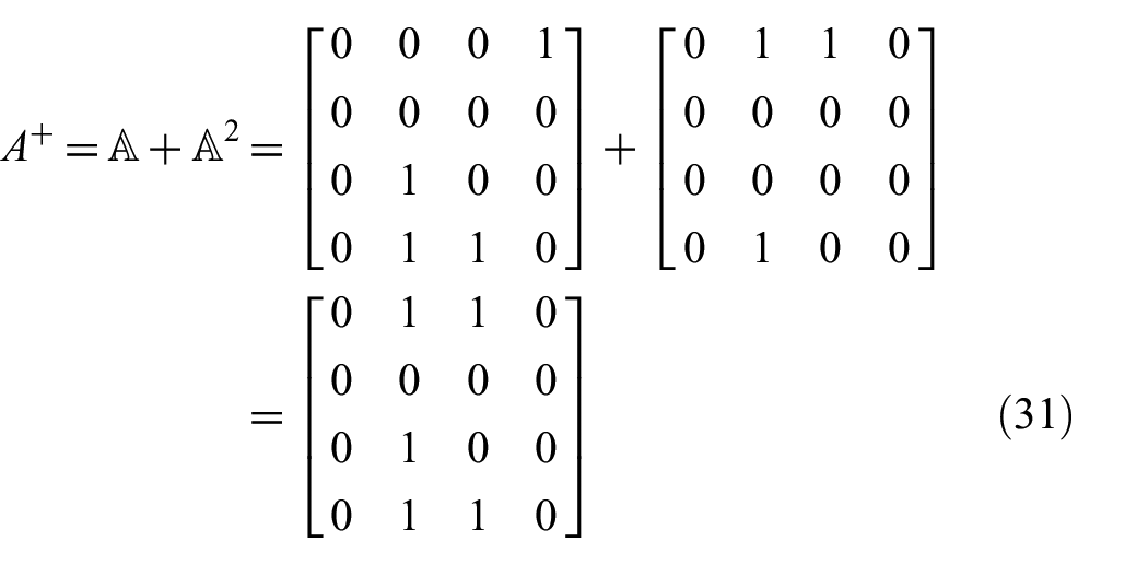
To determine attack reachability over any length of walk (attack depth), we can form the transitive closure of the attack graph. This expresses whether a given host is reachable (through any depth of walk) from another given host. We can write the transitive closure $A^{+}$ of adjacency matrix $A$ in terms of its Boolean matrix powers:

A^{+} = A + A^{2} + \dots A^{n - 1}

(10)

Here, each matrix power $A^{r}$ is computed via the Boolean matrix multiplication:

{[A^{2}]}_{i, j} = \lor_{k} a_{i, k} \land a_{k, j}

(11)

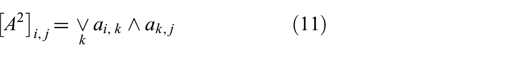
This has the same form as Equation (9), except the multiplication and addition operations are logical (Boolean) rather than arithmetic, that is, ∧ denotes the conjunction (logical AND) and ∨ denotes the disjunction (logical OR). Thus, Boolean matrix multiplication (and transitive closure) represents the presence of walks rather than the number of walks between a given pair of hosts. 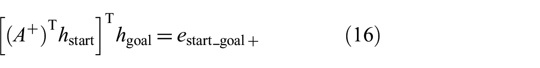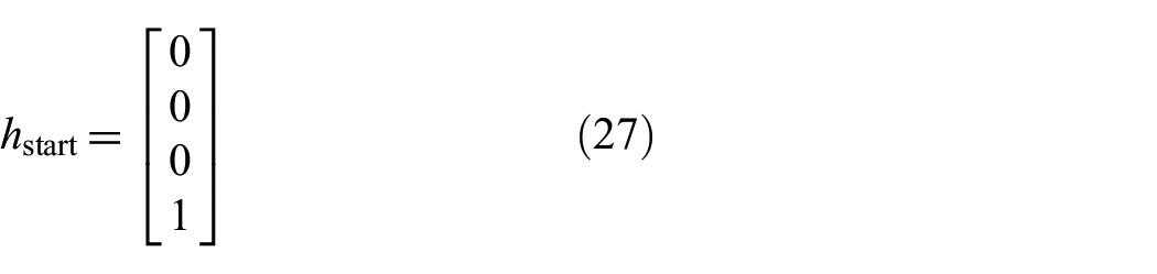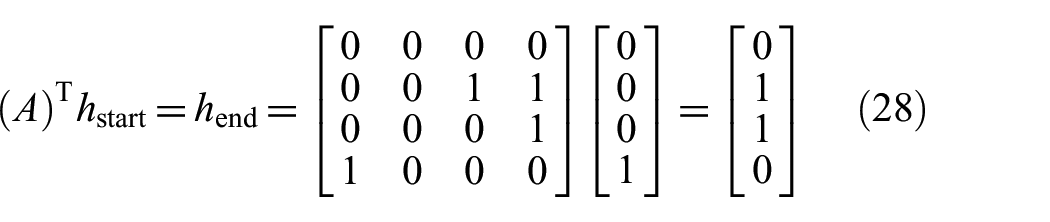That is, element $a_{i, j}^{+}$ of $A^{+}$ represents the reachability (through any depth of walk) from host $i$ to host $j$ , where $a_{i, j}^{+} = 1$ indicates the presence and $a_{i, j}^{+} = 0$ indicates the absence.

We can also apply matrix multiplication to determine attack reachability (numbers of walks of a given length) starting from a particular set of hosts. This provides additional information (beyond transitivity) for evaluating candidate policy solutions. For representing attack walks from each starting point using matrix multiplication, it is convenient to transpose the attack adjacency matrix:

{[A^{T}]}_{i, j} = {[A]}_{j, i}

(12)

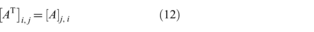
Recall our definitions of (attack and mission) adjacency matrices, that is, Equations (1) and (2). Here, elements of row $i$ of a matrix $A$ specify the outgoing edges for host $i$ , and elements of column $j$ specify the incoming edges for host $j$ . For the transpose $A^{T}$ , the rows represent the incoming edges, and the columns represent the outgoing edges. Then, when multiplying $A^{T}$ by a column vector for attack starting hosts, the elements of the columns (outgoing edges) for each row of $A^{T}$ align with the elements of the rows (in the usual sense for standard matrix multiplication) for the column vector representing starting hosts (i.e., giving outbound edges from starting hosts).

We define an $n \times 1$ (column) vector $h_{start}$ to represent the (one or more) attack starting host(s). Then, $h_{start i} = 1$ for host $i$ as a starting host, and $h_{start i} = 0$ otherwise. We can now apply the following:

A^{T} h_{start} = h_{end}

(13)

This yields the $n \times 1$ (column) vector $h_{end}$ , which represents direct (unity path length) reachability from each starting host. That is, $h_{end j} = 1$ represents that host $j$ is directly reachable from the starting host(s) defined in $h_{start}$ (i.e., those with $h_{start i} = 1$ ). Then, $h_{end j} = 0$ represents that ending host $j$ is not directly reachable from the starting host(s).

We can also define an $n \times 1$ (column) vector $h_{goal}$ to represent the (one or more) attack goal host(s), with $h_{goal i} = 1$ for host $i$ as a goal host, and $h_{goal i} = 0$ otherwise. Then, this expression computes $k_{start_goal}$ , that is, the number of direct (length 1) attack walks from starting host(s) to goal host(s):

{(A^{T} h_{start})}^{T} h_{goal} = k_{start_goal}

(14)

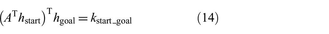
We can apply this kind of matrix multiplication for determining the number of attack walks (from start to goal) of a given length. We use the attack adjacency matrix of power $r$ to count the walks of a given length $r$ . This expression yields $k_{start_goal_r}$ , which is the number of length-r walks from the starting host(s) to the goal host(s):

{[{(A^{r})}^{T} h_{start}]}^{T} h_{goal} = k_{start_goal_r}

(15)

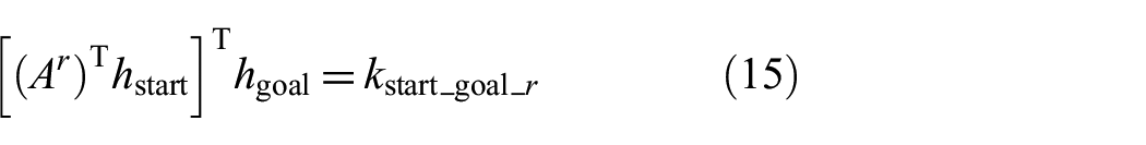
Using the transitive closure adjacency matrix, we can determine the existence of walks of any depth from attack start to goal:

{[{(A^{+})}^{T} h_{start}]}^{T} h_{goal} = e_{start_goal +}

(16)

For optimization fitness evaluation, we can determine the number of attack walks of length $r$ , from attack starts to attack goals, for a hardened attack graph $A'$ :

{[{({A'}^{r})}^{T} h_{start}]}^{T} h_{goal} = k'_{start_goal_r}

(17)

Depending on the instance of an optimization problem, there might be some policy rules (or combination of rules) that are infeasible as elements of a solution (e.g., that do not obey problem constraints). Or there might be security solutions that operate on rules in a certain way.

For example, a particular application might require certain hosts and services to be connected for the application to function properly, so that all those connections should be considered as a single “safety set” unit (rather than individually) in optimization. Another example (not employing microsegmentation) is that network-based firewalls are only able to enforce policy for traffic that is routed through them, so that optimization needs to consider only those vulnerable connections from one network segment to another (separated by a firewall).

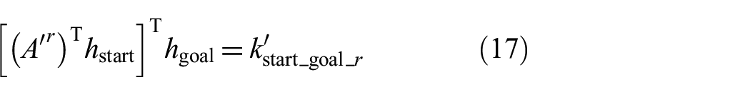
To represent such aggregations of individual security rules, we define a $1 \times q$ vector of $q$ security settings $C$ . An element $c_{k}$ of $C$ represents a set of elements (policy rules) ${p_{i_{1}, j_{1}}, p_{i_{2}, j_{2}}, \dots}$ of policy $P$ (in the simplest case, $c_{k}$ could represent an individual policy element $p_{i, j}$ ). For example, an element of $C$ could represent the allowance of a set of connections (safety set) for an application, or the allowance of a set of connections from one network segment to another (for a network-based firewall). The modeling of such security settings is incorporated in Albanese et al.,⁸ although that approach does not allow for resiliency tradeoffs (adversary thwarting vs mission availability) in policy optimization.

Figure 3 summarizes the relationships among security settings, policy rules, attack vectors (original and hardened), and mission needs (original and hardened). This figure also includes an optimization objective function $f (A', M')$ . This function represents one or more values that are to be optimized based on the policy-constrained attack vectors and policy rules.

Figure 3.

Elements of policy optimization problem space.

In our problem formulation, policy rules are determined by the security settings. We generally assume that $q < n^{2}$ , so that the search space of $O (2^{q})$ for security settings is smaller than the search space of $O (2^{n^{2}})$ for policy rules. So, in this framework, an algorithm for solving an optimization problem needs to search the space of security settings. A given combination of security settings forms a candidate solution to the problem. For a given candidate solution (combination of settings), the algorithm needs to apply the settings to the policy rules and apply the policy rules to the attack and mission graphs to harden them. Finally, the algorithm needs to evaluate the objective function for the candidate solution, and test whether the solution meets the problem constraints.

3.2. Ideal assumptions

We begin with a set of ideal assumptions, which form optimization constraints in terms of blocked attack paths and unblocked mission edges. This leads to the definition of a constrained optimization problem that minimizes the total number of blocked edges (that block attack paths and do not block mission edges).

Thus, we define the following constrained optimization problem:

Optimization Problem P1

(Objective O1) Minimize the number of blocked (denied) host-to-host edges such that (Constraint C1.1) no mission host pair is blocked and (Constraint C1.2) there exists no attack path from given attack start host(s) to given attack goal host(s).

Recall that for an attack graph with adjacency matrix $A$ and policy $P$ , the hardened attack graph $A'$ (i.e., $A$ with policy $P$ applied) is $A' = P ° A$ . We say that an attack path is blocked by the policy $P$ when that path does not exist in the hardened attack graph $A'$ , that is, if at least one of the edges of the attack path is blocked by that policy.

In Problem P1, we make the ideal assumptions that it is possible to block all attack paths from attack start(s) to attack goal(s) (i.e., Constraint C1.2) while simultaneously ensuring that no mission host pair (graph edge) is blocked (Constraint C1.1). Here, the sets of attack starting hosts and attack goal hosts are disjoint (non-overlapping); otherwise, we have a degenerate case in which the attack goal hosts are already compromised by the adversary.

For a policy rules graph $P$ , optimizing Objective O1 (minimizing the number of blocked edges, for which $p_{i, j} = 0$ ) corresponds to maximizing unblocked edges (for which $p_{i, j} = 1$ ). Thus, we can write Objective O1 as the following:

Objective O 1 : \max_{P} \sum_{i, j} p_{i, j}

(18)

Under Constraint C1.1, all mission edges are to be allowed via the policy rules $P$ , that is:

Constraint C 1.1 : m_{i, j} = 1 \Rightarrow p_{i, j} = 1

(19)

With the hardened attack graph $A'$ from Equation (6), and the given set of attack start hosts $a_{start}$ and set of attack goal hosts $a_{goal}$ , Constraint C1.2 can be written as:

Constraint C 1.2 : ∄ a'_{start} \to a'_{goal}

(20)

Here, $a \to b$ represents a path (sequence of alternating nodes and edges, with no repeated nodes or edges) from node $a$ to $b$ in the attack graph.

In the following sections, we examine illustrative examples of Optimization Problem P1. In section 3.2.1, we examine a particular instance of P1, in which there is a single optimal solution to this problem. In section 3.2.2, we examine a different instance of P1, in which the solution to this problem is non-unique (more than one solution yields the same value of the objective function).

3.2.1. Unique solution

This section examines a particular instance of Optimization Problem P1. As we show, this instance of P1 has a unique solution that optimizes Objective O1 while obeying Constraints C1.1 and C1.2.

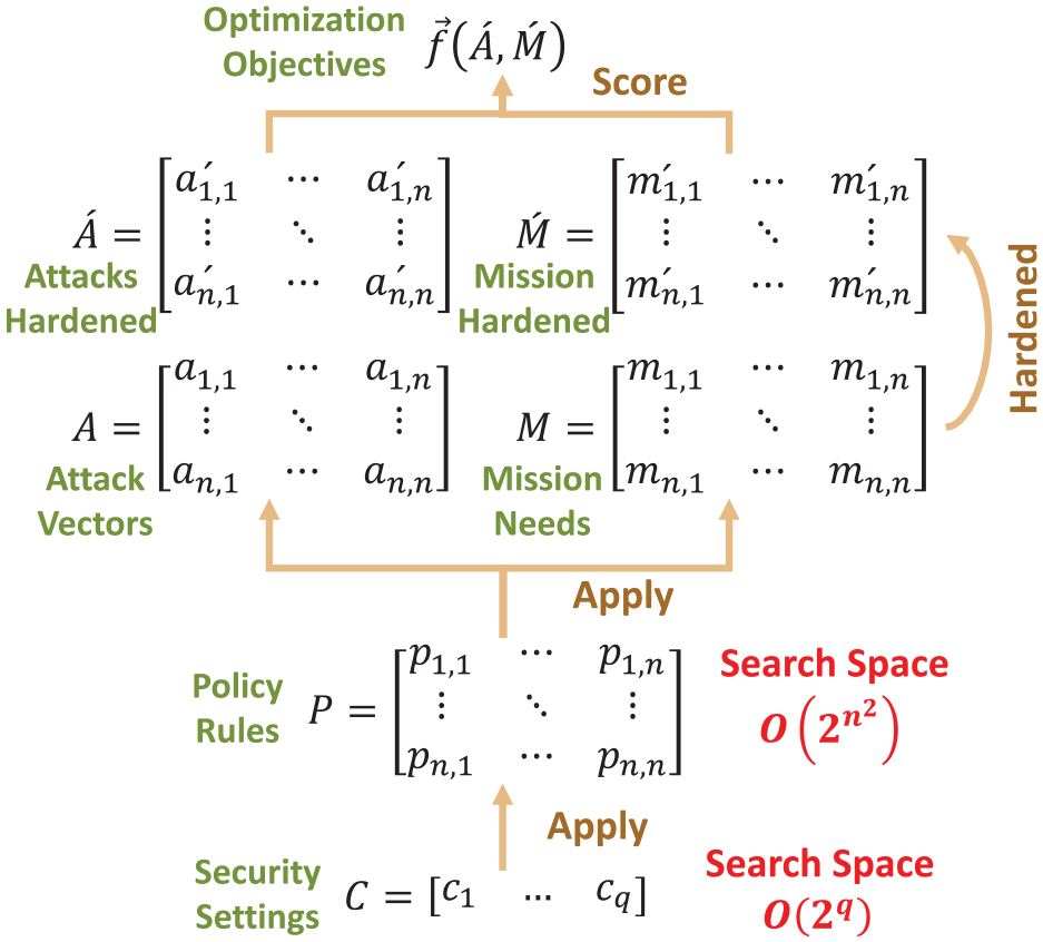
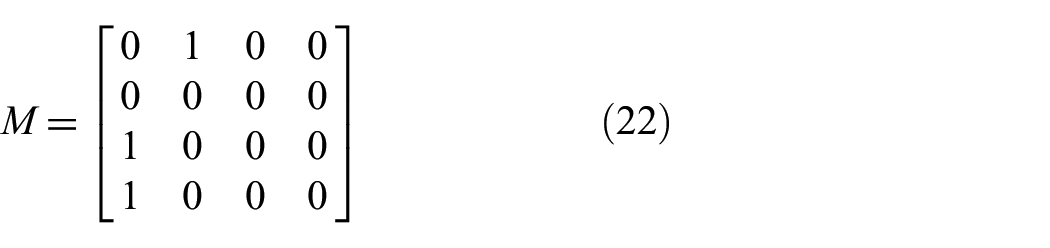
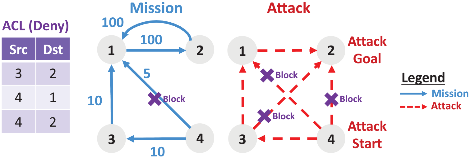
As shown in Figure 4, this instance of P1 has four network hosts. The graph nodes 1,…,4 represent these hosts. The blue (solid) graph edges represent host-to-host connectivity needed for the organizational mission. The red edges (dashed) represent the potential attacks from one host to another. The figure includes adjacency lists for the mission and attack edges (respectively).

Figure 4.

Example 1 (mission and attack edges).

As depicted in the figure, we assume that an attacker starts from Host 4, and seeks to compromise Host 2. That is, for Constraint C1.2 for this instance of P1, Host 4 is the attack start host ${\hat{a}}_{start}$ and Host 2 is the goal host ${\hat{a}}_{goal}$ .

Expressing the attack graph as a $4 \times 4$ binary adjacency matrix $A$ , we have:

A = [\begin{matrix} 0 & 0 & 0 & 0 \\ 0 & 0 & 0 & 0 \\ 0 & 0 & 0 & 0 \\ 0 & 1 & 1 & 0 \end{matrix}]

(21)

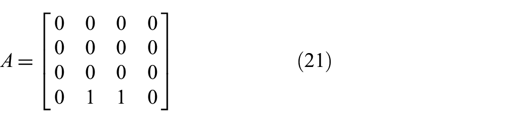
Expressing the mission graph as a $4 \times 4$ binary adjacency matrix $M$ , we have:

M = [\begin{matrix} 0 & 1 & 0 & 0 \\ 0 & 0 & 0 & 0 \\ 1 & 0 & 0 & 0 \\ 1 & 0 & 0 & 0 \end{matrix}]

(22)

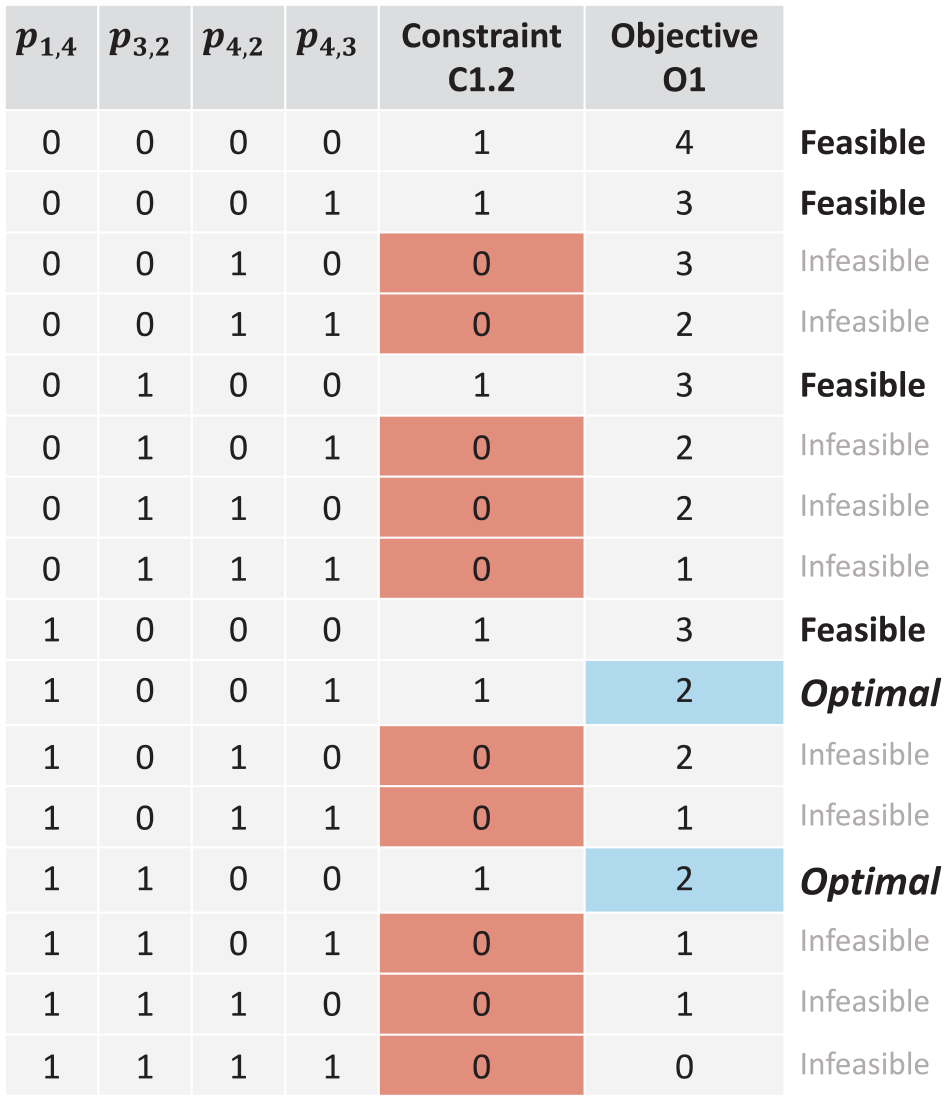
Optimization Problem P1 seeks a policy that minimizes the number of blocked edges (maximum number of unblocked edges). This is consistent with the constraint that no mission edges are blocked. Furthermore, only blocking edges in the attack graph will impact the existence of paths from Host 4 to Host 2 (the other constraint of P1). In the example of Figure 4, these attack-graph edges are $a_{4, 2}$ and $a_{4, 3}$ , which correspond to policy edges $p_{4, 2}$ and $p_{4, 3}$ (respectively). Any edges not in the attack graph $A$ can be assumed as unblocked in the potential policy rules graph $P$ , that is, $a_{i, j} = 0 \Rightarrow p_{i, j} = 1$ .

Taking these constraints into consideration, we have:

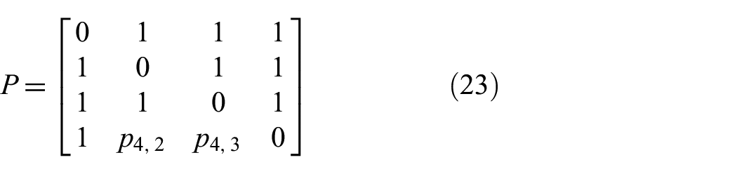
P = [\begin{matrix} 0 & 1 & 1 & 1 \\ 1 & 0 & 1 & 1 \\ 1 & 1 & 0 & 1 \\ 1 & p_{4, 2} & p_{4, 3} & 0 \end{matrix}]

(23)

This shows that there are only 2² = 4 combinations (binary values of $p_{4, 2}$ and $p_{4, 3}$ ) to be considered in solving this instance of Optimization Problem P1.

So, since $A$ gives one-step attacks, the value $a_{4, 2} = 1$ indicates that there is a direct attack path (one step) from Host 4 to Host 2. The optimal policy rules $\hat{P}$ must block that one-step attack, that is, ${\hat{p}}_{4, 2} = 0$ (which is feasible since mission edge $m_{4, 2} = 0$ ).

We next examine deeper paths, which could potentially lead from Host 4 to Host 2. Since $A^{2} = A^{3} = 0$ , there are no paths of length 2 or 3 (assuming no cycles, the maximum path length for a graph of $n$ nodes is $n - 1$ ). Since attack-graph edge $a_{4, 3}$ is not on any path (of any length) from Host 4 to Host 2, and there is no mission edge from Host 4 to Host 3 $(m_{4, 3} = 0)$ , and P1 seeks to minimize the number of blocked edges, the optimal policy rules $\hat{P}$ include ${\hat{p}}_{4, 3} = 1$ .

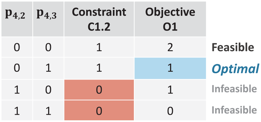
Figure 5 summarizes the optimization outcomes for each potential solution of this problem instance. For each combination of the values of $p_{4, 2}$ and $p_{4, 3}$ , the figure gives the truth value for Constraint C1.2 (no attack path from Host 4 to Host 2) and the number of blocked edges (Objective O1). In each case, Constraint C1.1 (no mission pair is blocked) is true, since $p_{4, 2}$ and $p_{4, 3}$ are independent of the mission edges.

Figure 5.

Candidate solutions for Example 1.

The combinations ${p_{4, 2} = 1, p_{4, 3} = 0}$ and ${p_{4, 2} = 1, p_{4, 3} = 1}$ are infeasible, because they violate C1.2 (allow an attack path from Host 4 to Host 2). The combinations ${p_{4, 2} = 0, p_{4, 3} = 0}$ and ${p_{4, 2} = 0, p_{4, 3} = 1}$ are both feasible. Between these two, ${p_{4, 2} = 1, p_{4, 3} = 0}$ is optimal because it blocks only one edge, while ${p_{4, 2} = 0, p_{4, 3} = 0}$ blocks two edges.

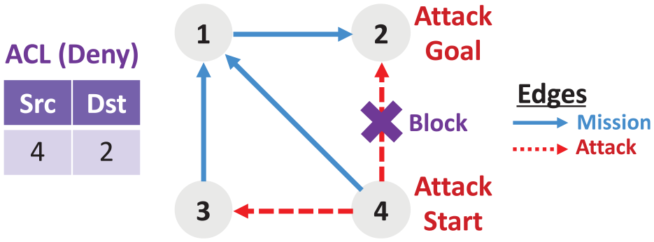
Figure 6 shows the optimal solution for this instance of Optimization Problem P1. For implementation (e.g., as an access control list), this corresponds to a “allow by default” (default binary ones of $\hat{P}$ ), with the “deny Host 4 to Host 2” rule.

Figure 6.

Optimal solution for Example 1.

3.2.2. Non-unique solutions

In the previous section, there is a single optimal solution for the given instance of Problem P1. In this section, we describe another instance of P1 that has more than one optimal solution, illustrating that optimal solutions are not necessarily unique.

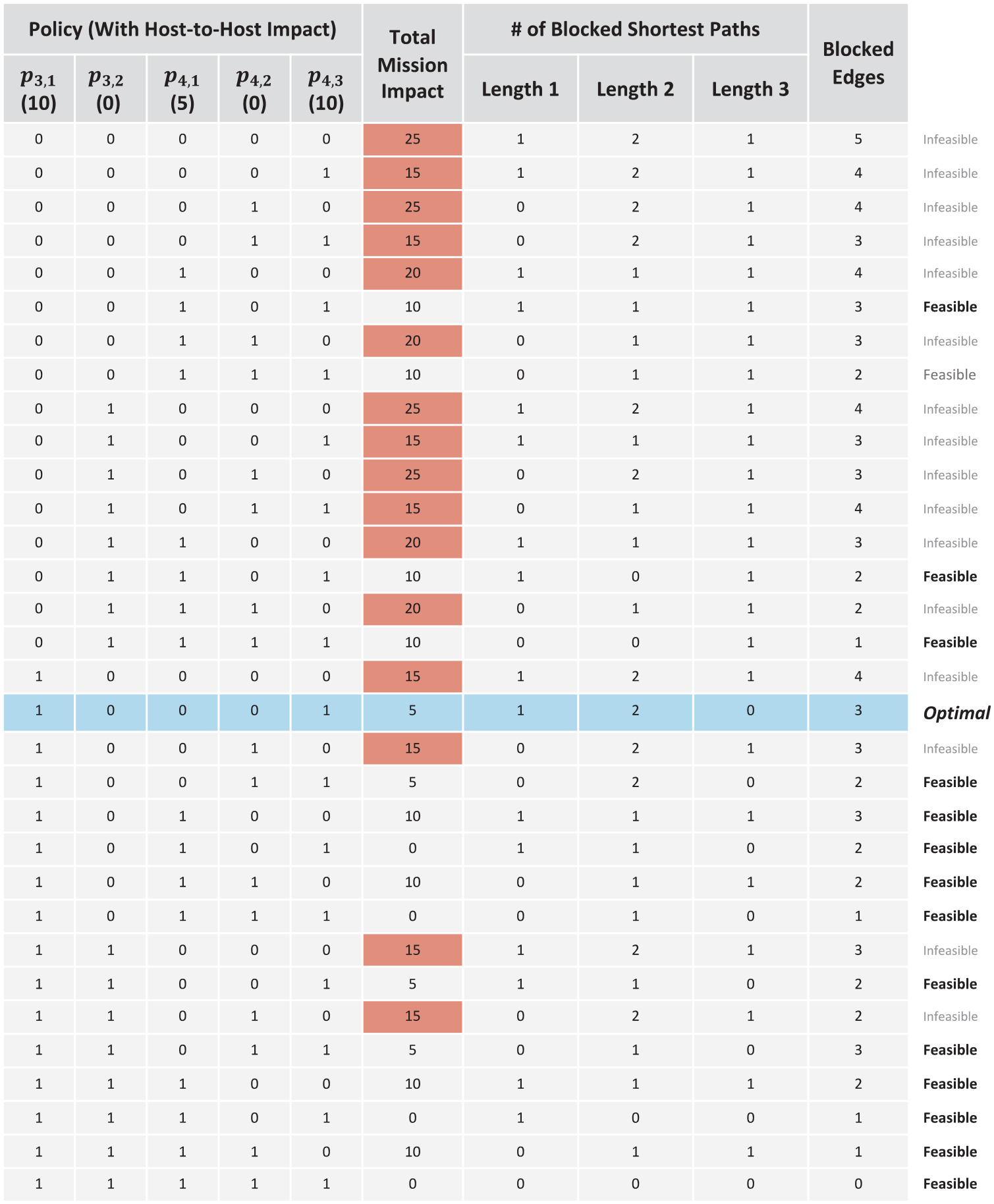
Consider the instance of Optimization Problem P1 in Figure 7. In comparison to Figure 4, this instance of P1 has two additional attack-graph edges: $a_{1, 4} = 1$ and $a_{3, 2} = 1$ .

Figure 7.

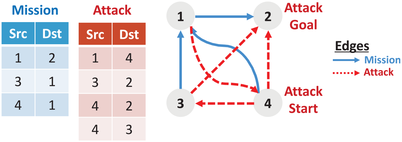
Example 2 (mission and attack edges).

The mission graph adjacency matrix $M$ is unchanged from Figure 4, that is:

M = [\begin{matrix} 0 & 1 & 0 & 0 \\ 0 & 0 & 0 & 0 \\ 1 & 0 & 0 & 0 \\ 1 & 0 & 0 & 0 \end{matrix}]

(24)

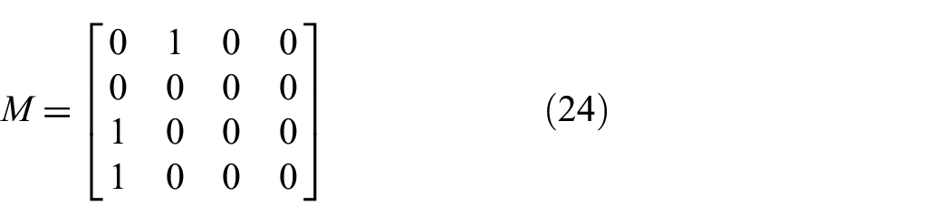
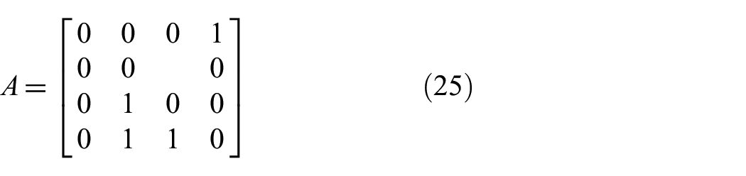
The attack graph adjacency matrix $A$ is now:

A = [\begin{matrix} 0 & 0 & 0 & 1 \\ 0 & 0 & 0 \\ 0 & 1 & 0 & 0 \\ 0 & 1 & 1 & 0 \end{matrix}]

(25)

As described in the previous section, the policy rules (blocked edges) $P$ under consideration are the edges in the attack graph $A$ . That is:

P = [\begin{matrix} 0 & 1 & 1 & p_{1, 4} \\ 1 & 0 & 1 & 1 \\ 1 & p_{3, 2} & 0 & 1 \\ 1 & p_{4, 2} & p_{4, 3} & 0 \end{matrix}]

(26)

This shows that there are now 2⁴ = 16 combinations (binary values of $p_{1, 4}$ , $p_{3, 2}$ , $p_{4, 2}$ , and $p_{4, 3}$ ) to be considered in solving this new instance of Optimization Problem P1.

To determine attack paths from the starting host (Host 4), we define the column vector $h_{start}$ :

h_{start} = [\begin{matrix} 0 \\ 0 \\ 0 \\ 1 \end{matrix}]

(27)

Applying Equation (13) to $A$ , we have:

{(A)}^{T} h_{start} = h_{end} = [\begin{matrix} 0 & 0 & 0 & 0 \\ 0 & 0 & 1 & 1 \\ 0 & 0 & 0 & 1 \\ 1 & 0 & 0 & 0 \end{matrix}] [\begin{matrix} 0 \\ 0 \\ 0 \\ 1 \end{matrix}] = [\begin{matrix} 0 \\ 1 \\ 1 \\ 0 \end{matrix}]

(28)

This shows that there are two length-1 attack walks from Host 4, ending at Host 2 and Host 3. Next, computing $A^{2}$ shows the number of length-2 attack walks between each host pair:

A^{2} = [\begin{matrix} 0 & 1 & 1 & 0 \\ 0 & 0 & 0 & 0 \\ 0 & 0 & 0 & 0 \\ 0 & 1 & 0 & 0 \end{matrix}]

(29)

Applying Equation (13), substituting $A^{2}$ for $A$ , we have:

{(A^{2})}^{T} h_{start} = h_{end} = [\begin{matrix} 0 & 0 & 0 & 0 \\ 1 & 0 & 0 & 1 \\ 1 & 0 & 0 & 0 \\ 0 & 0 & 0 & 0 \end{matrix}] [\begin{matrix} 0 \\ 0 \\ 0 \\ 1 \end{matrix}] = [\begin{matrix} 0 \\ 1 \\ 0 \\ 0 \end{matrix}]

(30)

This shows that there is one length-2 attack walk from Host 4, which ends at Host 2. Repeating this for $A^{3}$ shows that there are no length-3 walks starting from Host 4 in the attack graph.

Applying Equation (10), we find the transitive closure (binary reachability through walks of any length) for the attack graph $A$ :

\begin{matrix} A^{+} = A + A^{2} & = [\begin{matrix} 0 & 0 & 0 & 1 \\ 0 & 0 & 0 & 0 \\ 0 & 1 & 0 & 0 \\ 0 & 1 & 1 & 0 \end{matrix}] + [\begin{matrix} 0 & 1 & 1 & 0 \\ 0 & 0 & 0 & 0 \\ 0 & 0 & 0 & 0 \\ 0 & 1 & 0 & 0 \end{matrix}] \\ = [\begin{matrix} 0 & 1 & 1 & 0 \\ 0 & 0 & 0 & 0 \\ 0 & 1 & 0 & 0 \\ 0 & 1 & 1 & 0 \end{matrix}] \end{matrix}

(31)

We can then apply Equation (13), substituting $A'^{+}$ for $A$ , to evaluate attack reachability for the attack graph that has been hardened by a candidate solution. For example, here is reachability for $p_{1, 4} = p_{3, 2} = p_{4, 2} = p_{4, 3} = 0$ :

\begin{matrix} {({A'}^{+})}^{T} h_{start} & = {({[P ° A]}^{+})}^{T} h_{start} = h_{end} \\ = {({[[\begin{matrix} 0 & 1 & 1 & 0 \\ 1 & 0 & 1 & 1 \\ 1 & 0 & 0 & 1 \\ 1 & 0 & 0 & 0 \end{matrix}] ° [\begin{matrix} 0 & 0 & 0 & 1 \\ 0 & 0 & 0 & 0 \\ 0 & 1 & 0 & 0 \\ 0 & 1 & 1 & 0 \end{matrix}]]}^{+})}^{T} [\begin{matrix} 0 \\ 0 \\ 0 \\ 1 \end{matrix}] \\ = {({[\begin{matrix} 0 & 0 & 0 & 0 \\ 0 & 0 & 0 & 0 \\ 0 & 0 & 0 & 0 \\ 0 & 0 & 0 & 0 \end{matrix}]}^{+})}^{T} [\begin{matrix} 0 \\ 0 \\ 0 \\ 1 \end{matrix}] = 0 \end{matrix}

(32)

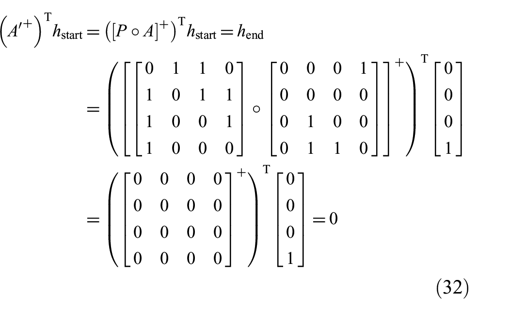
Figure 8 summarizes the optimization’ outcomes for each potential solution of this problem instance.

Figure 8.

Candidate solutions for Example 2.

For each combination of the values of $p_{1, 4}$ , $p_{3, 2}$ , $p_{4, 2}$ , and $p_{4, 3}$ , Figure 8 gives the truth value for Constraint C1.2 (no attack path from Host 4 to Host 2) and the number of blocked edges (the value to be optimized). In each case, Constraint C1.1 (no mission pair is blocked) is true, since $p_{1, 4}$ , $p_{3, 2}$ , $p_{4, 2}$ , and $p_{4, 3}$ are independent of the mission edges.

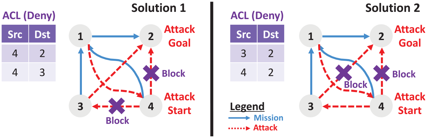
Figure 9 shows the optimal solutions for this instance of Optimization Problem P1. In this case, there is no unique optimal solution, that is, there are two solutions that are both feasible and have the minimum value of blocked edges (two). These optimal solutions are ${p_{1, 4} = 1, p_{3, 2} = 0, p_{4, 2} = 0, p_{4, 3} = 1}$ (Solution 1) and ${p_{1, 4} = 1, p_{3, 2} = 1, p_{4, 2} = 0, p_{4, 3} = 0}$ (Solution 2). For an access control list, this can be implemented as “allow by default” with either “deny Host 3 to Host 2 and deny Host 4 to Host 2” or “deny Host 4 to Host 2 and deny Host 4 to Host 3” rules.

Figure 9.

Optimal solutions for Example 2.

3.3. More realistic assumptions

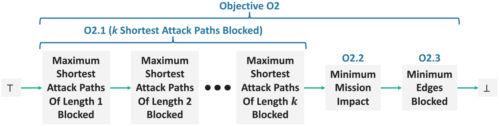
Next, we relax the ideal assumptions from the previous section to more realistic ones. Rather than insisting that no mission edges are blocked by policy rules, assume that we are given a budget for an allowed amount of mission impact. We also relax the constraint of blocking all attack paths to an optimization objective, that is, maximizing the number of blocked shortest paths. From these relaxed assumptions, we formulate a more realistic optimization problem, which maximizes resilience in terms of blocked attack paths within a given mission-impact budget.

We then define the following constrained optimization problem:

Optimization Problem P2

(Objective O2) In priority order, (Sub-Objective O2.1) maximizes the blocked shortest attack paths from attack start(s) to goal(s), (Sub-Objective O2.2) with minimum impact on the mission, (Sub-Objective O2.3) using the least number of blocked (deny) policy edges such that (Constraint C2) the mission impact is within a given budget.

For both attack and mission graphs, we consider the possibility that graph edges (representing host-to-host connectivity) are weighted. Edge weights are intended to represent the following:

For a mission graph, a weight for an edge represents the value of the edge to the organizational mission. For example, if an organization values high traffic volume as an indicator of mission need, the relative volume of traffic between hosts could be the mission edge weights.

For an attack graph, a weight for an edge represents the value of the edge in helping to thwart attacks. For example, the expected time to compromise one host from another could be the attack edge weights.

Sub-Objective O2.1 is a kind of shortest-paths problem. However, we are not merely interested in policies that only block the single shortest path from attack start to goal—that would leave other (longer) paths available for the attacker. At the other extreme, enumerating all paths is prohibitively expensive, since counting all graph paths from a start node to a goal node (the s–t paths problem) is #P complete (the analogue of NP completeness for counting problems).¹³ Also, while it is possible to estimate the number of s–t paths in a graph,¹⁴ we require the actual paths (not simply the number of paths) for evaluating O2.1.

We therefore define Sub-Objective O2.1 in terms of the k-shortest-paths problem.¹⁵ This problem is about finding the k-shortest paths from a start node $s$ to a target node $t$ in a directed weighted graph for an arbitrary natural number $k$ . Rather than specifying the actual value of $k$ in advance, we seek to evaluate shortest paths until some threshold value of a property is reached.¹⁶ We need only evaluate those k-shortest paths such that mission impact is within a given budget (Constraint C2) when the shortest paths are blocked. For handling multiple start nodes and/or multiple goal nodes, we can introduce a proxy start node and/or proxy goal node (as needed), where the proxy start node is connected to each actual start node, and each actual goal node is connected to the proxy goal node.

For a given shortest path $i$ in an attack graph, we write its path length (sum of edge weights along path $i$ ) as $l_{i}$ . We rank the shortest path lengths in ascending (most optimal to least optimal) order, that is, $l_{1} \leq l_{2} \dots \leq l_{k}$ . For a weighted attack graph (adjacency matrix) $A$ , the hardened attack graph $A'$ (i.e., $A$ with policy $P$ applied) is $A' = P ° A$ . We say that shortest attack path $i$ (in $A$ ) is blocked when path $i$ does not exist in the hardened attack graph $A'$ (i.e., its path length $l_{i} = \infty$ ). We denote such a blocked shortest attack path as $l_{i}^{blocked}$ . In terms of optimization, we define a dominance relation on the blocked paths, that is, $l_{i}^{blocked} ⪰ l_{i + δ}^{blocked}$ , for $δ > 0$ such that $i + δ \leq k$ . In other words, a solution is more optimal if it blocks an attack path of shorter length, which extends across all k-shortest paths. We denote solutions with the greater dominance-blocked attack paths as $l_{i}^{blocked ⪰}$ . Then Sub-Objective O2.1 is written as:

Sub - Objective O 2.1 : \max_{P} \sum_{i} l_{i}^{blocked ⪰}

(33)

Sub-Objective O2.2 seeks to minimize impact on the mission. For a weighted mission graph (adjacency matrix) $M$ , the hardened version $M'$ (i.e., $M$ with policy $P$ applied) is $M' = P ° M$ . Then, we say that a hardened mission edge (weight) $m'_{i, j}$ is impacted by policy $P$ when $p_{i, j} = 0$ (i.e., when the policy denies connectivity from host $i$ to host $j$ ). We denote such an impacted mission edge weight as $m_{i, j}^{impact}$ . Sub-Objective O2.2 is then written as:

Sub - Objective O 2.2 : \min_{M'} \sum_{i, j} m_{i, j}^{impact}

(34)

Sub-Objective O2.3 minimizes the number of blocked (deny) edges in the policy graph, independent of the attack and mission graphs. For a policy rules graph $P$ , minimizing the number of blocked edges (for which $p_{i, j} = 0$ ) corresponds to maximizing unblocked edges (for which $p_{i, j} = 1$ ). Thus, we can write Sub-Objective O2.3 as the following:

Sub - Objective O 2.3 : \max_{P} \sum_{i, j} p_{i, j}

(35)

The overall Objective O2 is defined in terms of dominance relations among Sub-Objectives O2.1, O2.2, and O2.3, that is:

Objective O 2 : O 2.1 ≻ O 2.2 ≻ O 2.3

(36)

This denotes that for Objective O2, Sub-Objective O2.1 (shortest attack paths blocked) dominates the other two sub-objectives, and that Sub-Objective O2.2 (minimum mission impact) dominates Sub-Objective O2.3 (minimum policy edges blocked). So, for example, if Solution A is better than Solution B in terms of O2.1, then Solution A is more optimal, regardless of O2.2 and O2.3 for either solution. Or, if Solutions A and B have the same O2.1 optimality, and Solution A is better than Solution B in terms of O2.2, then Solution A is more optimal.

These dominance relations are depicted in Figure 10. Here, we assume that attack path edges have unit weight. Thus, blocked shortest paths of unit length dominate shortest paths of length 2, and so on.

Figure 10.

Dominance relations among optimization objectives (Problem P2).

Consider the instance of Optimization Problem P2 in Figure 11. In this example, we are given a budget of 10 units for allowed mission impact (Constraint C2).

Figure 11.

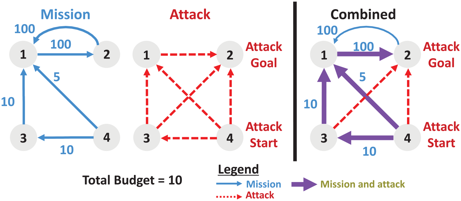
Example 3 (mission and attack edges).

Here is the weighted mission graph adjacency matrix $M$ :

M = [\begin{matrix} 0 & 100 & 0 & 0 \\ 100 & 0 & 0 & 0 \\ 10 & 0 & 0 & 0 \\ 5 & 0 & 10 & 0 \end{matrix}]

(37)

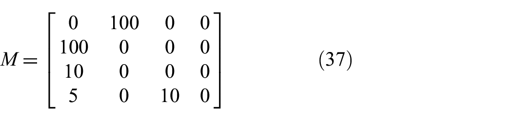
Here is the attack graph adjacency matrix $A$ (unit weights for attack reachability):

A = [\begin{matrix} 0 & 1 & 0 & 0 \\ 0 & 0 & 0 & 0 \\ 1 & 1 & 0 & 0 \\ 1 & 1 & 1 & 0 \end{matrix}]

(38)

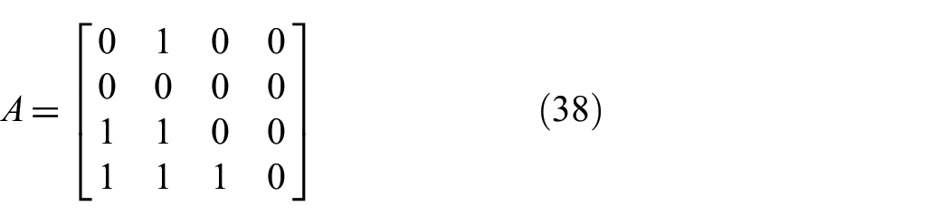
The policy rules (blocked edges) $P$ under consideration are the edges in the attack graph $A$ . Moreover, since mission edges $m_{1, 2}$ and $m_{2, 1}$ exceed the mission-impact budget, they must remain unblocked in the policy, that is, $p_{1, 2} = p_{2, 1} = 1$ . Thus, as evaluated in Figure 12, there are 2⁵ = 32 host-to-host policy combinations to be considered for this instance of Optimization Problem P2:

P = [\begin{matrix} 0 & 1 & 1 & 1 \\ 1 & 0 & 1 & 1 \\ p_{3, 1} & p_{3, 2} & 0 & 1 \\ p_{4, 1} & p_{4, 2} & p_{4, 3} & 0 \end{matrix}]

(39)

Figure 12.

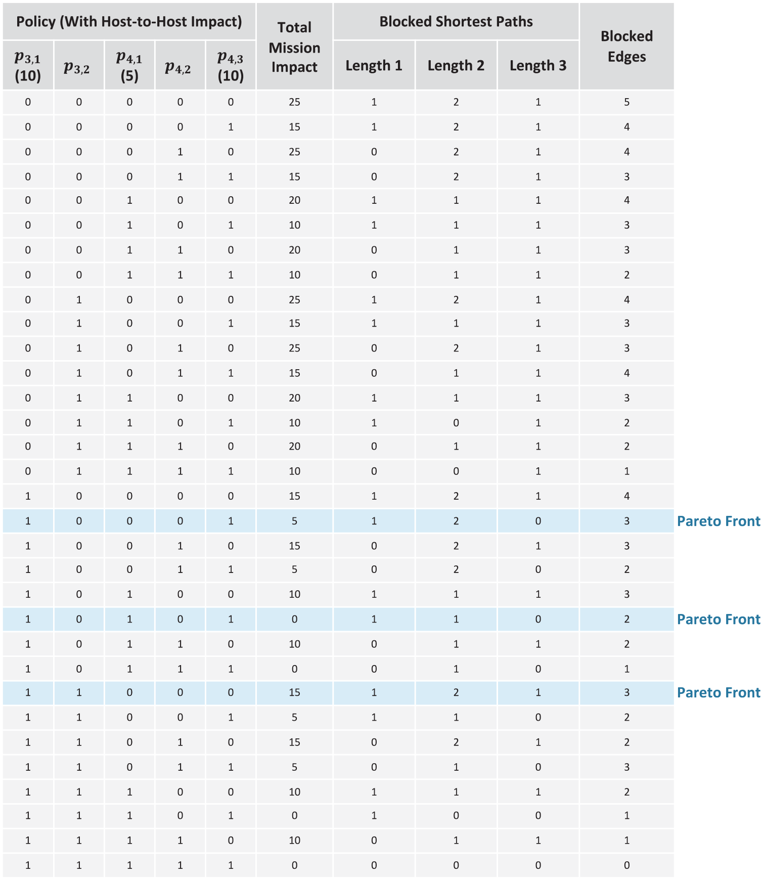
Candidate solutions for Example 3.

For each of these 32 policy combinations, Figure 12 shows the blocked shortest attack paths (Sub-Objective O2.1), mission impact (Sub-Objective O2.2), and blocked policy edges (Sub-Objective O2.3). Mission-impact values that exceed the budget of 10 units are marked in red (infeasible). The resulting optimal solution is marked in blue.

In this problem instance, here are the attack paths to be blocked, in dominance order (length of attack path):

Length-1 path (1): Host 4 → Host 2.

Length-2 paths (2):

Host 4 → Host 1 → Host 2.

Host 4 → Host 3 → Host 2.

Length-3 path (1): Host 4 → Host 3 → Host 1 → Host 2.

In Figure 12, there is a column for the numbers of shortest paths of each length that are blocked by a given policy combination. Since the attack-graph edges are assigned unit (equal) weights, blocking attack paths of equal length have equal optimality.

Figure 13 shows the optimal solution for this instance of Optimization Problem P2. This solution is ${p_{3, 1} = 1, p_{3, 2} = 0, p_{4, 1} = 0, p_{4, 2} = 0, p_{4, 3} = 1}$ .

Figure 13.

Optimal solution for Example 3.

3.4. Multi-objective optimization

Next, we relax the mission-impact budget constraint, and cast it as a second optimization objective. The resulting multi-objective optimization problem allows a Pareto-optimal tradeoff between security (attack resilience) and mission needs (impact from blocked hosts).

This leads to the following constrained multi-objective optimization problem:

Optimization Problem P3

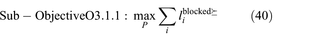
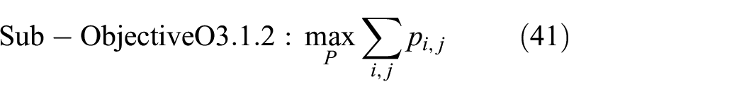
(Objective O3.1) Maximize (Sub-Objective O3.1.1) the blocked shortest paths from attack start(s) to attack goal(s), (Sub-Objective O3.1.2) using the least number of blocked (deny) policy edges. (Objective O3.2) Minimize the impact on the mission.

As for Problem P2, we assume that the (host-to-host) edges of the attack and mission graphs are weighted (for thwarting attacks and supporting the mission, respectively). Sub-Objective O3.1.1 is the same as Sub-Objective O2.1 (section 3.3), that is, maximizing blocked shortest attack paths:

Sub - Objective O 3.1.1 : \max_{P} \sum_{i} l_{i}^{blocked ⪰}

(40)

Sub-Objective O3.1.2 is the same as Sub-Objective O2.3 (section 3.3), that is, minimizing blocked edges (maximizing unblocked edges) in the policy graph, independent of the attack and mission graphs:

Sub - Objective O 3.1.2 : \max_{P} \sum_{i, j} p_{i, j}

(41)

The overall Objective O3.1 is defined in terms of dominance relations among Sub-Objectives O3.1.1 and O3.1.2:

Objective O 3.1 : O 3.1.1 ≻ O 3.1.2

(42)

This denotes that for Objective O3.1, Sub-Objective O3.1.1 (shortest attack paths blocked) dominates Sub-Objective O3.1.2 (minimum policy edges blocked). So, for example, if Solution A is better than Solution B in terms of O3.1.1, then Solution A is more optimal, regardless of O3.1.2 for either solution. Or, if Solutions A and B have the same O3.1.1 optimality, and Solution A is better than Solution B in terms of O3.1.2, then Solution A is more optimal.

Objective O3.2 is the same as Sub-Objective O2.2 (section 3.3), that is, minimizing mission impact from the application of a policy:

Objective O 3.2 : \min_{M'} \sum_{i, j} m_{i, j}^{impact}

(43)

Figure 14 shows the dominance relations between O3.1.1 and O3.1.2 (for Objective O3.1). Objective O3.2 is a separate objective in Problem P3, which shows as non-dominated in the partial order in Figure 14. In the figure, it is assumed that attack path edges have unit weight. Thus, blocked shortest paths of unit length dominate shortest paths of length 2, and so on.

Figure 14.

Dominance relations among optimization objectives (Problem P3).

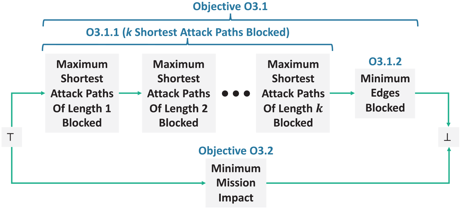
Figure 15 depicts how the dominance relations among elements of Sub-Objectives O3.1.1 and O3.1.2 can be implemented as numerical ranges, so that Objective O3.1 can be weighted along with O3.1. The scheme in Figure 15 maps the numbers of allowed shortest paths from attack starts to attack goals to a particular range for each path length.

Figure 15.

Mapping dominance relations of optimization objectives to numerical ranges.

For a given candidate solution, the number of blocked paths (or walks, if computed via matrix multiplication) of length 1 is mapped to the range of $1 / 2$ (no length-1 walks blocked) to 1 (all possible length-1 walks blocked). Similarly, the number of walks of length 2 is mapped from $1 / 4$ (no length-2 walks blocked) to $1 / 2$ (all possible length-2 walks blocked). This continues through some maximum number of walk lengths under consideration (in Figure 15, through walks of length 4).

This pattern of mapping numbers of progressively longer walks to progressively smaller numerical ranges yields overall objective fitness numbers that rank candidate solutions according to the priority (dominance relation) defined in Objective O3.1.1. The last part of this dominance-relation mapping is to map the total number of unblocked edges to the remaining range (Objective O3.1.2), that is, for a maximum walk length of 4, from zero (no edges unblocked) to $1 / 16$ (all edges unblocked). This smallest range yields solutions that have fewer overall blocked edges for a given number of blocked adversarial walks from attack starts to goals.

We now examine an instance of Optimization Problem P3, using Example 3 in Figure 11 of section 3.3. Since Problem P3 does not have a mission-impact constraint (budget), the budget shown in Figure 11 does not apply.

As before, the blocked edges in policy $P$ under consideration are the edges in the attack graph $A$ given in Equation (38). However, since Problem P3 has no mission-impact budget constraint (as in Problem P2), we must include all six of the attack-graph edges in the combination of policy rules over which we optimize (2⁶ = 64 combinations):

P = [\begin{matrix} 0 & p_{1, 2} & 1 & 1 \\ 1 & 0 & 1 & 1 \\ p_{3, 1} & p_{3, 2} & 0 & 1 \\ p_{4, 1} & p_{4, 2} & p_{4, 3} & 0 \end{matrix}]

(44)

Figure 16 evaluates five of these six attack-graph edge combinations (i.e., $p_{3, 1}$ , $p_{3, 2}$ , $p_{4, 1}$ , $p_{4, 2}$ , and $p_{4, 3}$ ) for optimality (2⁵ = 32 combinations). The figure only has combinations for which $p_{1, 2} = 1$ (unblocked). Since blocking connectivity from Host 1 to Host 2 has a mission impact of 100 units, while not blocking any attack paths already blocked by other solutions with lower mission impact, those other solutions dominate ones in which $p_{1, 2} = 0$ (blocked) and are omitted in the figure.

Figure 16.

Candidate solutions of Problem P3 for Example 3.

In multi-objective optimization, a solution is called Pareto optimal if none of its objectives can be improved without worsening some of its other objectives.¹⁷ A Pareto front is a set of solutions that are Pareto optimal. In terms of dominance relations, a Pareto front is a set of non-dominated solutions, that is, for which no objective can be improved without sacrificing at least one other objective. A Pareto front identifies set of candidate solutions (e.g., from among a larger set of dominated solutions) for analyzing tradeoffs among conflicting objectives. Figure 16 marks the Pareto front resulting from evaluating candidate solutions to this instance of Problem P3. The candidate solutions evaluated in Figure 16 are plotted in Figure 17.

Figure 17.

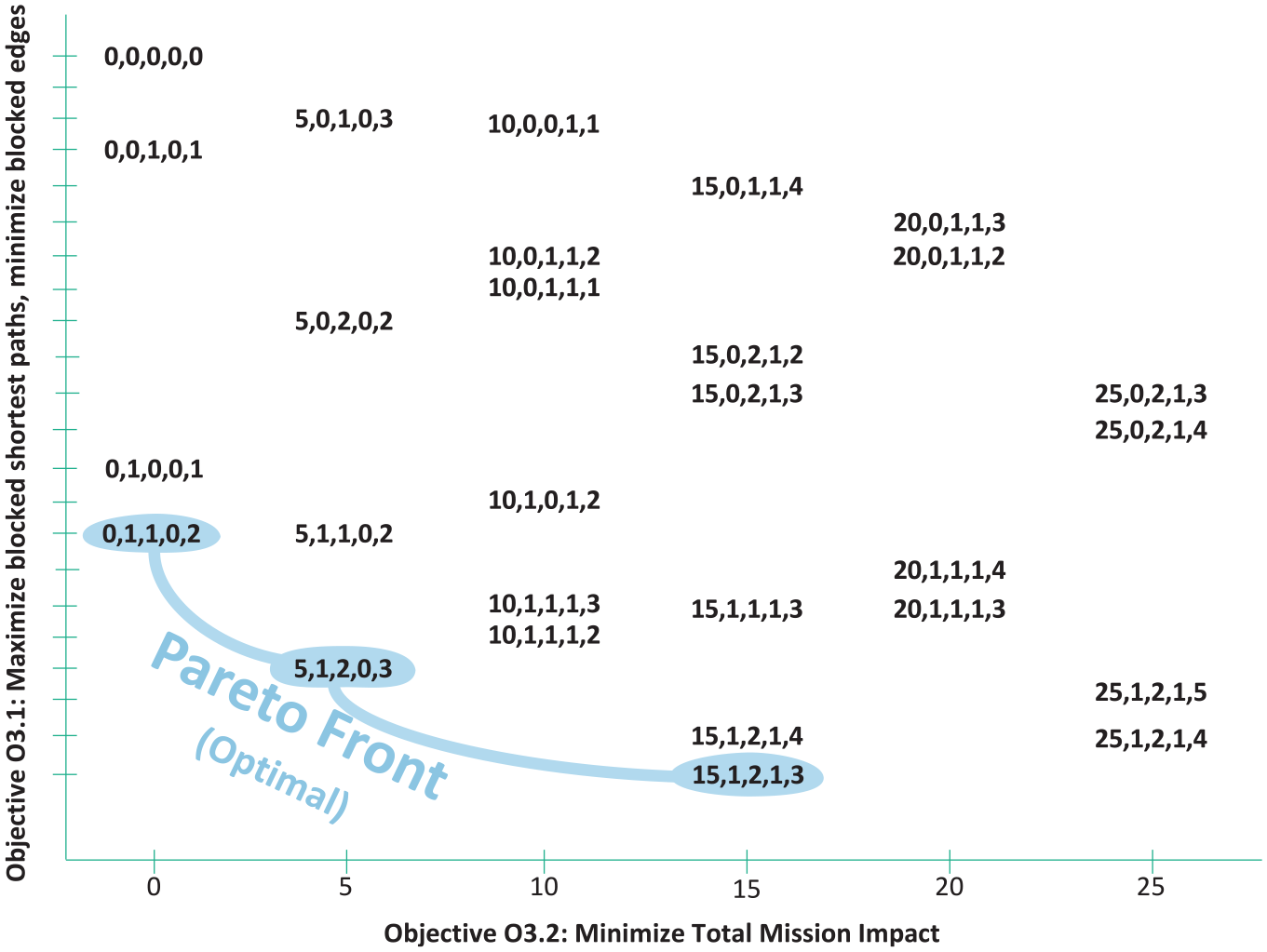
Candidate solutions of Problem P3 for Example 3 (Pareto front).

In Figures 16 and 17, each solution is written in terms of its values for mission impact, blocked shortest paths, and blocked edges. In these figures, the candidate solutions are plotted in two dimensions, that is, Objective 3.1 (maximize blocked shortest paths, minimize blocked edges) and Objective 3.2 (minimize total mission impact).

Figure 18 shows the application of the three Pareto-optimal solutions in Figure 17 to the mission and attack graphs.

Figure 18.

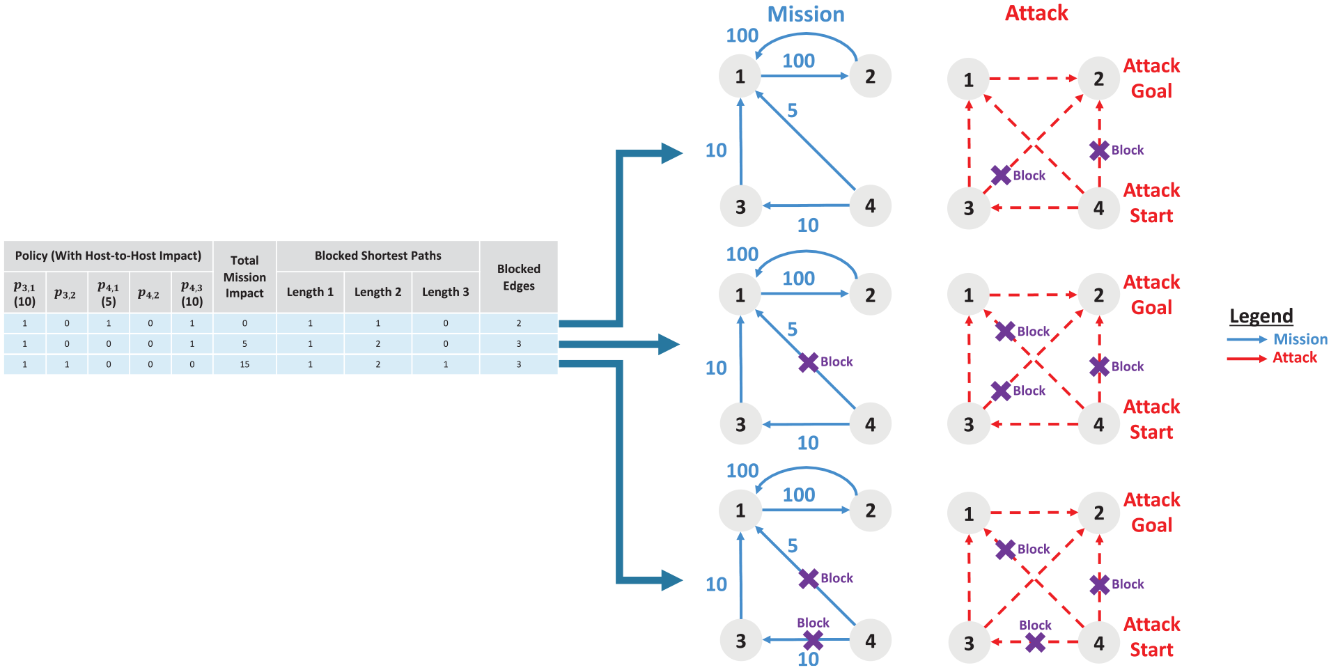
Pareto-optimal solutions of Problem P3 for Example 3.

4. Experimentation

In our approach, data from a network to be defended are collected, correlated, and used to build a graph-based model for potential multi-step lateral movement through the network. Figure 19(a) shows such a model, built from observed network traffic for a baseline (non-optimized) representative enterprise network within the ARES testbed.

Figure 19.

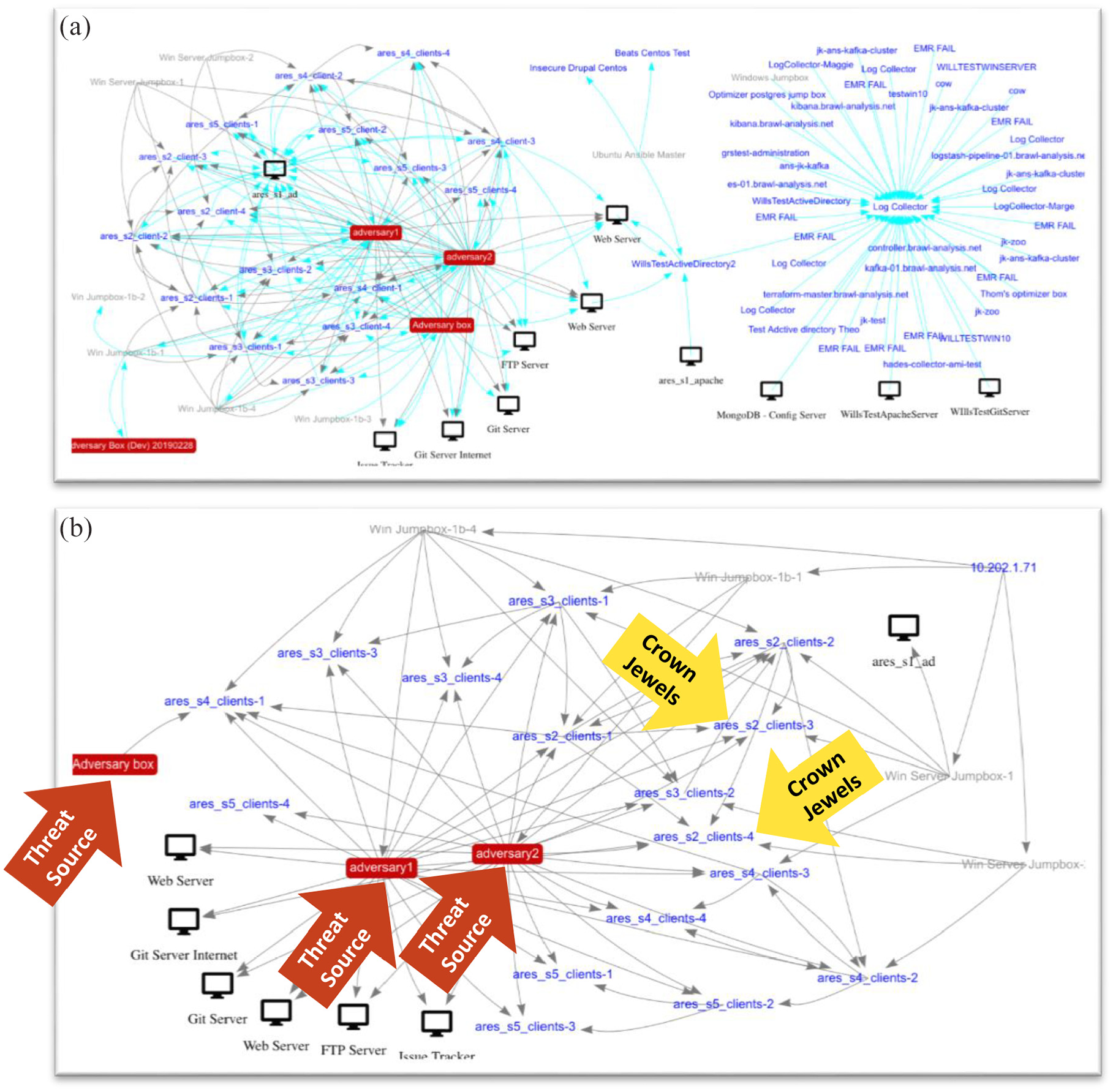
Baseline policy model for testbed network, including (a) the full graph from observed network traffic and (b) its vulnerable subgraph.

In Figure 19, graph nodes are network hosts and edges represent the set of all network flows for a given source and destination host. Edges are colored dark (black) if they include at least one (known) vulnerable service on the destination host; otherwise, edges are light colored (blue). Figure 19(b) shows the vulnerable subgraph for this network, that is, only those nodes and edges with at least one vulnerable service reachable from source host to destination host.

In the network of Figure 19, an adversary group (the ARES red team) has an initial presence on three hosts (red rectangles) in a validation exercise. In this exercise, the threat situation is that the red team starts from their initial presence, that is, the hosts marked threat source in Figure 19(b), and then moves laterally through the network until reaching the two hosts marked crown jewels.

In Figure 20(a), the graph is constrained to include only those vulnerable edges that lie between the threat sources (attack starts) and the crown jewels (attack goals). This represents the potential adversary lateral movement (attack paths) for this threat situation. Note that for this attack graph, there are paths from only two of the three attack starts that lead to the goals.

Figure 20.

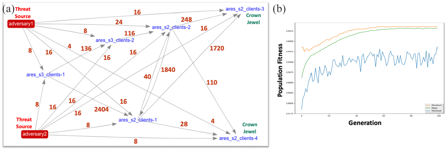
Optimizing microsegmentation policy over a threat/mission situation, including (a) the vulnerable graph that lies between assumed attack starts and goals and (b) genetic algorithm convergence to an optimal solution.

In Figure 20(a), the graph edges are also labeled with numbers indicating the total mission criticality for all network flows represented by each edge. There are various approaches, for example, Rebovich et al.,¹⁸ Musman et al.,¹⁹ Heinbockel et al.²⁰ and Schulz et al.²¹ and others for analyzing and quantifying such mission dependency/criticality for network assets. In this experiment, we apply these mission criticality weights to the corresponding terms (denied edges) in the mission-impact summation defined for Sub-Objective O3.1.2 (section 3.4).

The network model and threat/mission situation in Figure 20(a) then forms the input for our optimization of microsegmentation policy. We apply evolutionary programming in the form of a genetic algorithm²² to learn the optimal policy. In the genetic algorithm, each individual in a population represents a candidate solution to the optimization problem. Each candidate solution is a particular combination of allowed or denied edges in the network model. At each step of simulated evolution, the genetic algorithm selects individuals for reproduction based on how well they meet the objective (fitness) defined in section 3.4, that is, maximizing a given level of tradeoff between adversary effort and access to mission resources for the given threat/mission situation.

Figure 20(b) shows statistics for fitness values over time as the genetic algorithm population evolves to an optimal solution. In this case, there are 88 vulnerable edges (exploitable from attack starts to attack goals) in the attack graph. Thus, the overall search space of combinations of allowed/denied edges (policy instances) for this attack graph is 10²⁶. The genetic algorithm execution time in this case is 14 s, for evolution over 100 generations, with a population size of 400, and tournament selection with a tournament size of two.

Figure 21 shows the resulting optimal policies computed by the genetic algorithm, for six different relative weights between maximizing adversary effort (Objective O3.1) and maximizing mission accessibility (Objective O3.2) in the fitness function. In the figure, the red (thicker) edges indicate that the vulnerable connections from source to destination are denied in the policy. The gray (thinner) edges indicate that all connections are allowed from source to destination, even the vulnerable ones.

Figure 21.

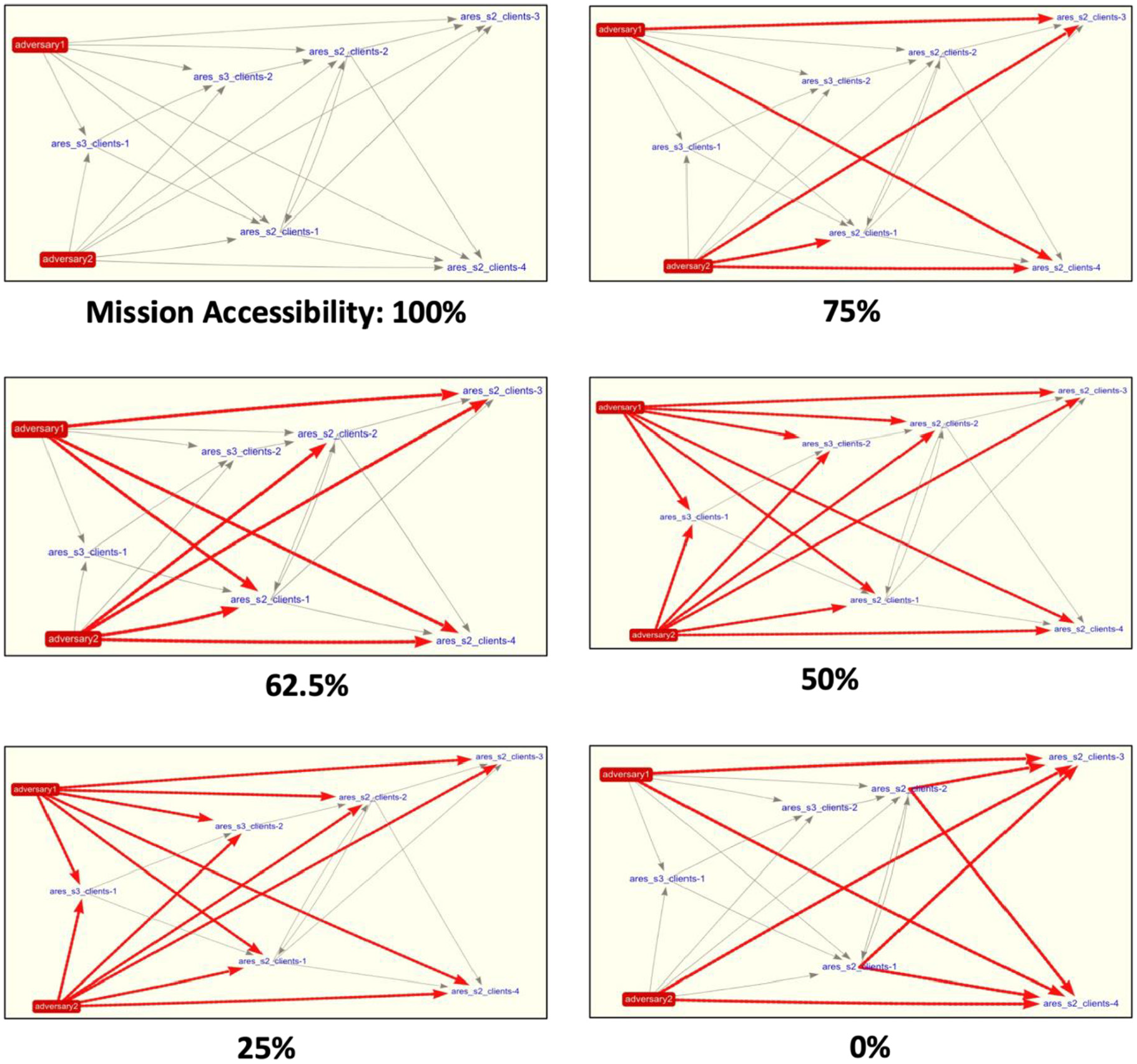
Optimal policies for different usability vs security tradeoffs.

In Figure 21, when mission accessibility is weighted 100%, the optimal policy is to allow all edges. This is because blocking an edge makes it unavailable for the organizational mission, but no emphasis is placed on how the blocked edge contributes to increasing the adversary effort. Then, as less emphasis is placed on mission accessibility (e.g., as the threat becomes more severe), there is an optimal tradeoff for a given relative weighting between usability and security, with additional emphasis on maximizing adversary effort resulting in additional blocked edges. In each case, edges that support shorter exploitation paths (from attack starts to goals) and have lower mission criticality are preferentially blocked versus other edges. Then, at the other extreme, when the emphasis is fully on maximizing adversary effort, the optimal policy is to block all paths from attack starts to attack goals, using the minimum number of blocked edges (Objective O3.1.2 from section 3.4), since mission accessibility (Objective O3.2) has no impact on policy optimization.

Figure 22 shows the number of denied vulnerable edges for optimal policies via our genetic algorithm, sampling across the range of relative weights between maximizing adversary effort (Objective O3.1) and maximizing mission accessibility (Objective O3.2). This shows the discrete nature of this problem, that is, how particular optimal solutions span a range of weight values, switching to another solution when the fitness function crosses a particular threshold value.

Figure 22.

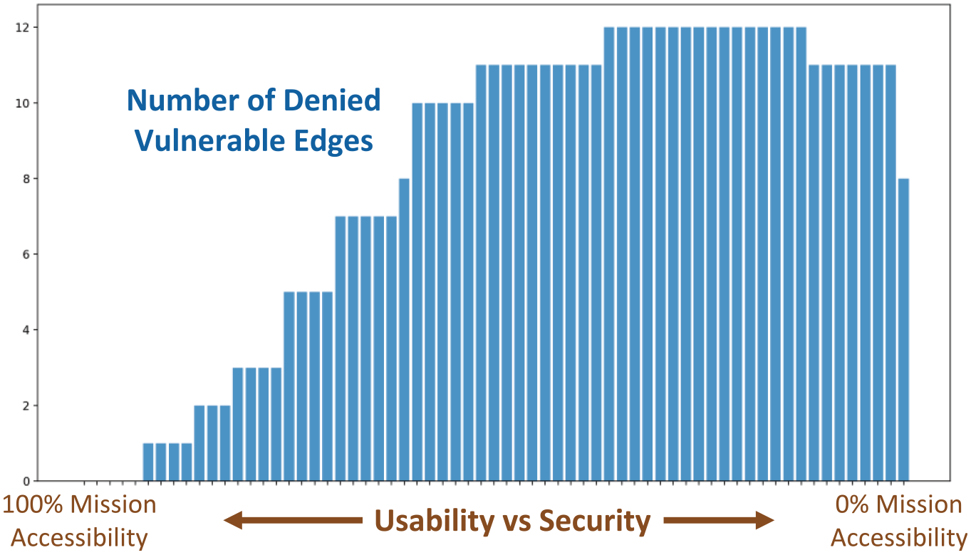
Full range of tradeoff between usability and security.

Operationally, our synthesized microsegmentation policies are enforced via AWS security groups. This acts as a virtual host-based firewall for each AWS Elastic Compute Cloud (EC2) instance.²³ A deployed policy is comprised of security group rules controlling inbound and outbound traffic for each EC2 instance. This provides access control at the network transport layer (source/destination IP addresses, source/destination ports, and protocols). We then conduct ongoing red teaming exercises within a testbed environment to assess the efficacy of synthesized policies.

Figure 23 shows run times for our microsegmentation policy optimization for networks of various sizes. The run times are for a MacBook Pro with a 2.6 GHz 6-Core Intel Core i7 processor and 32 GB 2400 MHz DDR4 memory.

Figure 23.

Performance for computing optimal microsegmentation policy.

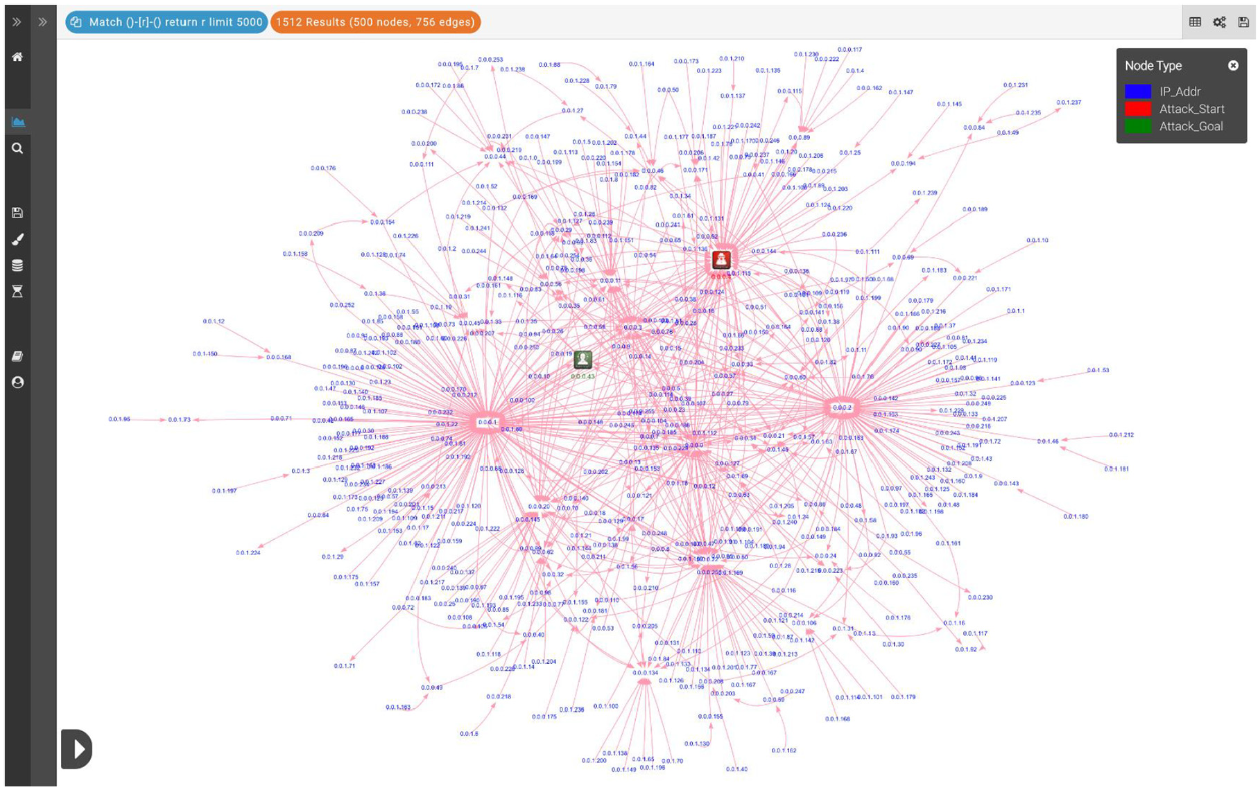
For the results in Figure 23, the data for each network are synthesized via a generative model that learns statistical distributions from our live testbed environment (comprised of 74 hosts). While the details are omitted for brevity, we apply a genetic algorithm that learns the parameters of a scale-free generative model that provides the best fit to our live network data, as measured by triadic census. This generative model provides the ability to generate data sets of arbitrary scale for such performance testing. Figure 24 shows traffic flows for the three synthesized network data sets used as inputs for the optimization run times in Figure 23.

Figure 24.

Synthesized networks for optimization performance testing.

In Figure 24, the host nodes (as blue text) represent the host IP addresses. Each edge (gray line) represents the presence of one or more flows from a source address to a destination address in the generated flow data. In these synthesized networks, based on the statistical model learned from our live network, there is a core region with densely interconnect hosts, with sparsely connected hosts on the periphery.

The visualizations in Figure 24 represent all flow data synthesized by our generative model (for a given optimization performance test). In the synthesized data sets, certain edges (from source to destination IP address) have at least one flow to a vulnerable service on the destination. In the optimization fitness function, such edges represent potential lateral movement by an adversary. Figure 25 shows the vulnerable subset of edges (shown as red lines) for the 500-host synthesized data set.

Figure 25.

Vulnerable edges (potential lateral movement) for 500-node network.

The fitness function also considers a given attack scenario, in which a set of hosts is defined as potential attack starting points and another set of hosts is defined as attack goals (e.g., critical hosts prioritized for protection). In Figure 25, those hosts are marked with Threat Actor (red) and Victim Target (for attack start and goal hosts, respectively) icons from the Structured Threat Information eXpression (STIX^™) language. Figure 26 shows the paths through the paths of potential lateral movement through the vulnerable subgraph of Figure 25, that is, leading from attack start host to attack goal host.

Figure 26.

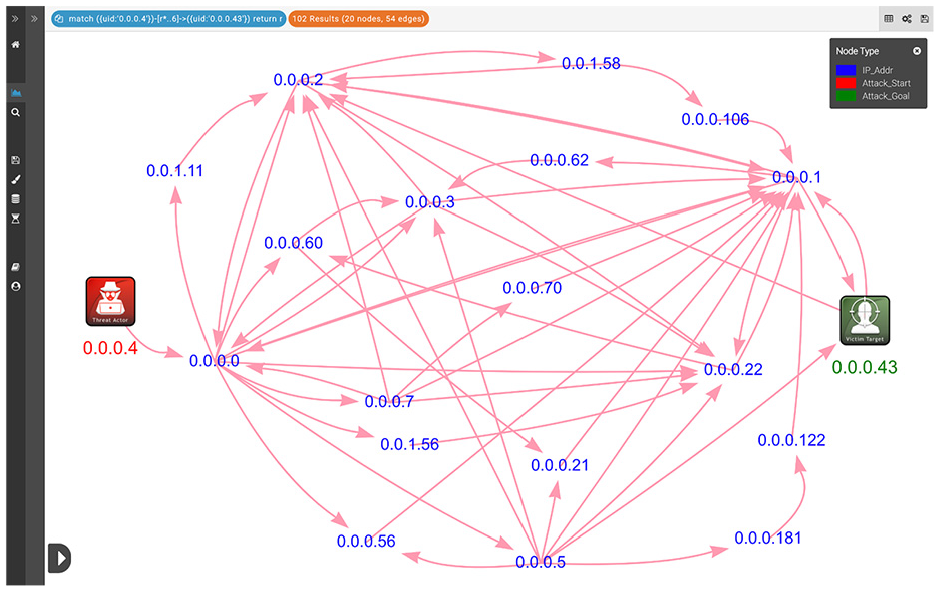
Potential lateral movement for assumed attack scenario (500-node network).

5. Summary

This paper describes an approach for synthesizing optimal network microsegmentation policy, with tunable tradeoffs between security and usability. For this, we formulate a novel optimization objective function that balances the need to maximize adversary effort (minimize cyberattack risks) while maximizing accessibility to critical network resources. We then apply this objective function for learning the optimal microsegmentation policy for a network through AI techniques (genetic algorithms).

Our objective function quantifies attacker reachability in terms of multi-step exploitation (lateral movement) through a network. We estimate the effort needed for an adversary to carry out a particular attack scenario, given the application of a particular candidate microsegmentation policy. This measures the extent to which a candidate policy solution blocks particular paths of exploitation, with a bias toward blocking shorter (less adversary effort) paths. We also measure the extent to which a given policy solution imposes restrictions on access to mission-critical services. These two measures (adversary effort and mission accessibility) support the balance between security and usability in our overall policy optimization objective function.

Our approach to cyber resiliency optimization leverages the fine level of granularity provided by microsegmentation, for limiting potential adversarial movement within a network. Our optimized microsegmentation policies are part of the MITRE Adaptive Resiliency Experimentation System (ARES), which jointly optimizes microsegmentation, authentication, policy generalization, redundancy, deception, and zero-trust architecture for adaptive intelligent cyber resiliency.

Footnotes

Funding

The author(s) received no financial support for the research, authorship, and/or publication of this article.

ORCID iD

Steven Noel

Author biographies

Steven Noel is a Principal Cybersecurity Scientist within the Cyber Solutions Innovation Center at The MITRE Corporation, McLean, Virginia, USA. A MITRE employee since 2013, Dr. Noel supports MITRE’s Science and Technology Portfolio for the US Army.

Vipin Swarup is a Distinguished Cybersecurity Engineer within the Cyber Solutions Innovation Center at The MITRE Corporation, McLean, Virginia, USA. A MITRE employee since 1990, Dr. Swarup supports the Threat Analysis and Mitigation Portfolio for MITRE’s Center for Securing the Homeland.

Karin Johnsgard is a Lead Multi-Discipline Systems Engineer within the Software Engineering Innovation Center at The MITRE Corporation, Aberdeen, Maryland, USA. A MITRE employee since 2001, Dr. Johnsgard supports MITRE’s Intelligence & Sensors Portfolio for the US Army.

References

United States Army Training and Doctrine Command (TRADOC). The US Army in multi-domain operations, 2028. Pamphlet 525-3-1, 6 December 2018. Fort Eustis, VA: TRADOC.

Bodeau

Graubart

. Cyber resiliency engineering framework. Technical report MTR110237, September 2011. McLean, VA: The MITRE Corporation.

Linkov

Eisenberg

Plourde

, et al. Resilience metrics for cyber systems. Environ Syst Decis 2013; 33: 471–476.

Ross

Pillitteri

Graubart

, et al. Developing cyber resilient systems: a systems security engineering approach, vol. 2 (Special publication no. 800-160). Gaithersburg, MD: National Institute of Standards and Technology (NIST), 2019.

Klein

Micro-segmentation: securing complex cloud environments. Netw Secur 2019; 2019: 6–10.

Program Executive Office Command Control Communications-Tactical (PEO C3T). Command post computing environment, https://peoc3t.army.mil/mc/cpce.php (accessed 20 November 2020).

Noel

A review of graph approaches to network security analytics. In: Samarati

Ray

(eds) From database to cyber security (Lecture notes in computer science). Cham: Springer, 2018, pp. 300–323.

Albanese

Jajodia

Noel

(inventors). Methods and systems for determining hardening strategies. Patent 9,203,861, USA, 1 December 2015.

Million

The Hadamard product, 2007, http://buzzard.ups.Edu/courses/2007spring/projects/million-paper.pdf (accessed 28 November 2018).

10.

Noel

Jajodia

Understanding complex network attack graphs through clustered adjacency matrices. In: Proceedings of the 21st annual computer security applications conference (ACSAC), Tucson, AZ, 5–9 December 2005.

11.

Kepner

Gilbert

Graph algorithms in the language of linear algebra. Philadelphia, PA: Society for Industrial and Applied Mathematics (SIAM), 2011.

12.

Weisstein

EW.

Matrix multiplication, http://mathworld.wolfram.com/MatrixMultiplication.html (accessed 30 November 2018).

13.

Valiant

LG.

The complexity of enumeration and reliability problems. SIAM J Comput 1979; 8: 410–421.

14.

Roberts

Kroese

DP.

Estimating the number of s–t paths in a graph. J Graph Algorithm Appl 2007; 11: 195–214.

15.

Eppstein

Finding the k shortest paths. SIAM J Comput 1998; 28: 652–673.

16.

Aljazzar

Leue

K^∗: a heuristic search algorithm for finding the k shortest paths. Artif Intell 2011; 175: 2129–2154.

17.

Miettinen

Nonlinear multiobjective optimization. New York: Springer Science+Business Media, 1998.

18.

Rebovich

Cormier

Norman

, et al. Systems engineering guide. McLean, VA: The MITRE Corporation, 2014.

19.

Musman

Tanner

Temin

, et al. A systems engineering approach for crown jewels estimation and mission assurance decision making. In: Proceedings of the IEEE symposium on computational intelligence in cyber security, Paris, 11–15 April 2011, pp. 210–216. New York: IEEE.

20.

Heinbockel

Noel

Curbo

. Mission dependency modeling for cyber situational awareness. In: Proceedings of the NATO IST-148 symposium on cyber defence situation awareness, Sofia, 3–4 October 2016, pp. 5.1–5.14. North Atlantic Treaty Organization Science and Technology Organization.

21.

Schulz

O’Gwynn

Kepner

, et al. Dynamically correlating network terrain to organizational missions. In: Proceedings of the NATO IST-153/RWS-21 workshop on cyber resilience, Munich, 23–25 October 2017, pp. 1–5. CEUR Workshop Proceedings.

22.

Fortin

De Rainville

Gardner

, et al. DEAP: evolutionary algorithms made easy. J Mach Learn Res 2012; 13: 2171–2175.

23.

Amazon Web Services (AWS). Elastic compute cloud, 2020, https://aws.amazon.Com/ec2/ (accessed 17 November 2020).