
Abstract
Multi-agent systems are of ever-increasing importance in a contested space environment—use of multiple, cooperative satellites potentially increases positive mission outcomes on orbit, while autonomy becomes an ever-increasing requirement to increase reaction time to dynamic situations and lower the burden on space operators. This research explores multi-agent satellite swarm Guidance, Navigation, and Control (GNC) using deep reinforcement learning (DRL). DRL policies are trained to provide guidance inputs to agents in multi-agent swarm environments for completing complex, teamwork-focused objectives in geosynchronous orbit. An example scenario is explored for a group of satellite agents maneuvering to triangulate an object that is non-stationary in the relative orbit frame. Reward shaping is used to encourage learning guidance that positions swarm members to maximize triangulation accuracy, using angles-only observations for navigation relative to the target. Results show the policies successfully learn guidance through reward shaping to improve triangulation accuracy by a significant factor.
Keywords
1. Introduction
As the space domain has become increasingly competitive, contested, and congested, the United States Space Force (USSF) has been created to meet new strategic needs. 1 Efforts to increase onboard autonomy for spacecraft Guidance, Navigation, and Control (GNC) are necessary to improve the ability to react quickly to complex situations in the future. Current operations are planned in advance by humans and would place a heavy burden on operators or become infeasible in the case of many satellites participating in a scenario simultaneously. 2 As multi-agent space systems and scenarios increase in scale, so will the difficulty of pre-planned maneuvers for multiple satellites. Looking to the future, AI solutions are of interest to the USSF for complex scenario possibilities including many agents. 3
Satellite swarming refers to a system of multiple agents that collectively work together toward an objective. Swarms will require GNC for an arbitrarily large number of vehicles in formations or arrangements based on relative or localized information. 4 Previous approaches to swarm-based space GNC rely heavily on heuristic approaches,5,6 relative orbital element (ROE)7,8 or natural motion circumnavigation (NMC) formations,9,10 and bounded scenarios.11,12 Machine learning is a fast-moving field, and recently, DRL has shown the ability to solve previously unsolvable problems and adapt to dynamic situations, including displaying super-human capability in multiplayer games with extremely large decision spaces. 13 DRL has the potential to greatly benefit the area of space control going forward.
This work explores the potential for DRL in the application of multi-agent satellite swarms in cooperative proximity operations. Recent research has shown the potential for other similar GNC applications such as satellite docking. 14 The potential for multi-agent cooperative play applied to the space domain is discussed here, inspired by examples such as OpenAI Five. 13
A relative dynamics environment at geosynchronous orbit using the well-known Hill Clohessy–Wiltshire (HCW) equations 15 is simulated. A policy for controlling swarm members is trained in a multi-agent environment using reward shaping for completing objectives that would be difficult for traditional GNC systems. In this paper, multiple satellites are tasked with triangulating the position of a moving target over a 12-h simulated period, and rewarded for learning to maneuver in ways that minimizes error in the triangulated position.
Electro-optics simulations are conducted to create realistic sensor data, and three different quality levels of sensors are discussed—a powerful star tracker suited for a large satellite, a smaller star tracker potentially available for a CubeSat platform, and a sensor with low-quality specifications equivalent to a cell phone camera that could potentially be used on a nano-scale satellite platform. Angle noise and probability of detection from the sensor simulations are used during triangulation calculations.
Multiple training runs are performed with different numbers of satellites in the randomized simulation and compared. The best trained policy is used in a variety of evaluation scenarios ranging from ideal to challenging conditions and results are compared. In addition, training techniques are also implemented to demonstrate fuel conservation learning and the effect on policy performance.
2. Related work
Reinforcement learning has risen to prominence over the past decade, as increases in computational power and research breakthroughs have given rise to DRL agents solving previously unsolvable problems. DRL agents have succeeded in outplaying humans in many spaces with highly complex decision spaces such as Atari, 16 the game of Go, 17 and even cooperative team-based games such as DOTA2. 13 While games provide a convenient space for research due their well-known rules and environments, controlling agents in games is just another GNC problem. This history of success in games, including multi-agent and teamwork-based examples, suggests that DRL techniques might be well suited for cooperative swarm-based GNC scenarios.
Swarming generally refers to an arbitrarily large numbers of agents acting based on local information to complete an objective together. Historically, when exploring swarms in the space domain, heuristic control laws have been used to form regular arrangements; 4 while there is an advantage of easily scaling to large numbers, this type of GNC limits the swarm to rigid, predetermined arrangements that do not suit a large variety of scenarios. Other examples of GNC design focused on maintaining specific formation between members include miniature phasing maneuvers or artificial potential functions. 10
Swarming can be approached both as a control optimization problem and a tasking and scheduling problem. Multi-agent optimal assignment and control using model-predictive control 6 allows for changes in the task to be enforced during execution using a receding finite horizon. Another method of assignment and control is using greedy heuristics for assigning passive relative orbits to members and incorporates dynamic programming for control design. 18
There has also been recent research on swarms in differential games non-specific to space, such as a cooperative pursuit. 19 This approach solves the game of multiple pursuers and a single evader mathematically by directing the pursuers to minimize the area of the evader’s Voronoi partition.
Reinforcement learning applications for space-based proximity operations has also seen a variety of recent research. Sargent et al. 20 compare the previous multi-agent pursuit game with DRL policies trained in the same scenario and seek to create a classifier using DRL that identifies the GNC technique correctly as either a DRL algorithm or traditional optimization-based approach.
Hovell and Ulrich 14 use DRL to train a policy on guidance strategy that feeds a conventional controller to track and dock with a rotating spacecraft. Using this separation in GNC parts, the research demonstrates a lowered learning burden can better allow transfer from simulation to reality with a hardware-based experiment showing comparable performance. While not using space-based physics for simulation, the learning was successfully transferred to robots moving in two dimensions in a controlled environment. The scenarios included challenging docking approaches such as docking with a spinning target and while avoiding an obstacle.
In the work by Lei et al., 21 a multi-agent satellite inspection problem is explored using DRL with two joint policies in a hierarchal approach. Three satellites are tasked to cooperate and fully inspect the surface of an object that is stationary in the local-vertical, local-horizontal (LVLH) frame—to do so, a higher-level policy chooses from 20 predetermined inspection points surrounding the target at a fixed distance, while a lower-level policy thrusts the agent to the chosen point. The hierarchal framework successfully drove the satellites to inspect the target in a distant-efficient fashion, but the target was assumed to be stationary and did not avoid inspection or maneuver otherwise.
Angles-only navigation, while not a primary focus of this work, is employed for the observations passed to the agents and therefore related works in the field should be studied. In the work by Kaplan, 22 various solutions for determining the position, velocity, or attitude of an observer are discussed using triangulation. A common trait in angles-only-based GNC is using multiple observations or known trajectories to determine the state of an observer, or inversely the observed. Specific to spacecraft, Kruger and D’Amico 23 propose navigation of multiple objects in a swarm by taking multiple observations from a removed observer and applying a multi-hypothesis tracking technique. In addition to using multiple observations, the use of ROEs to describe periodic relative motion is common in this application and does not suit the scenarios discussed in this work where trajectories of both the observers and observed may be constantly changing.
While there is much research on swarm formations, cooperative pursuit, and the use of angles-only measurements for GNC, there lies a gap in swarm applications for complex missions that involve non-stationary objectives or unbounded and dynamically changing scenarios.
3. Methodology
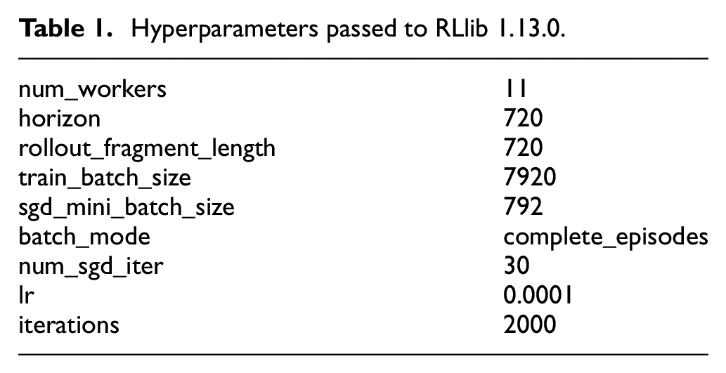
In order to facilitate fast RL training, a containerized software stack is used. RLlib 1.13.0 24 implements Proximal Policy Optimization (PPO) 25 training algorithm, handles all configuration and hyperparameters, and scales parallelized workers during training. OpenAI Gym 26 is used to build the environment that is loaded and stepped through each episode of training. The artificial neural networks (ANNs) for deep learning are implemented using TensorFlow. 27 The term agent refers to each of two or more satellites being controlled individually in the simulation, while the policy refers to the trained logic that each agent follows—only one policy is trained during a simulation run, and all agents have the same goal and use the same policy to choose actions based on observations to maximize reward. Initial exploratory experiments are conducted on a single workstation with 12 processor threads and 48 GB of memory. A training experiment with 11 workers for 2000 iterations typically averages a 6-h run time. Hyperparameters for the initial trials that have been changed from the defaults of RLlib 1.13.0 are listed in Table 1.
Hyperparameters passed to RLlib 1.13.0.
In this section, the simulation physics for the on-orbit environment are detailed, as well as the method for simulating and calculating triangulation for the primary metric of success. In addition, the method and parameters of DRL training in this simulation environment are described, along with the hyperparameters chosen and the reward shaping experimented with to train minimizing error on the triangulation metric.
3.1. Simulation environment
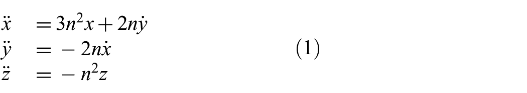
The well-known HCW equations shown in Equation (1) are used for the simulation states of all objects in the environment each step. No perturbations are included in the simulation dynamics, and
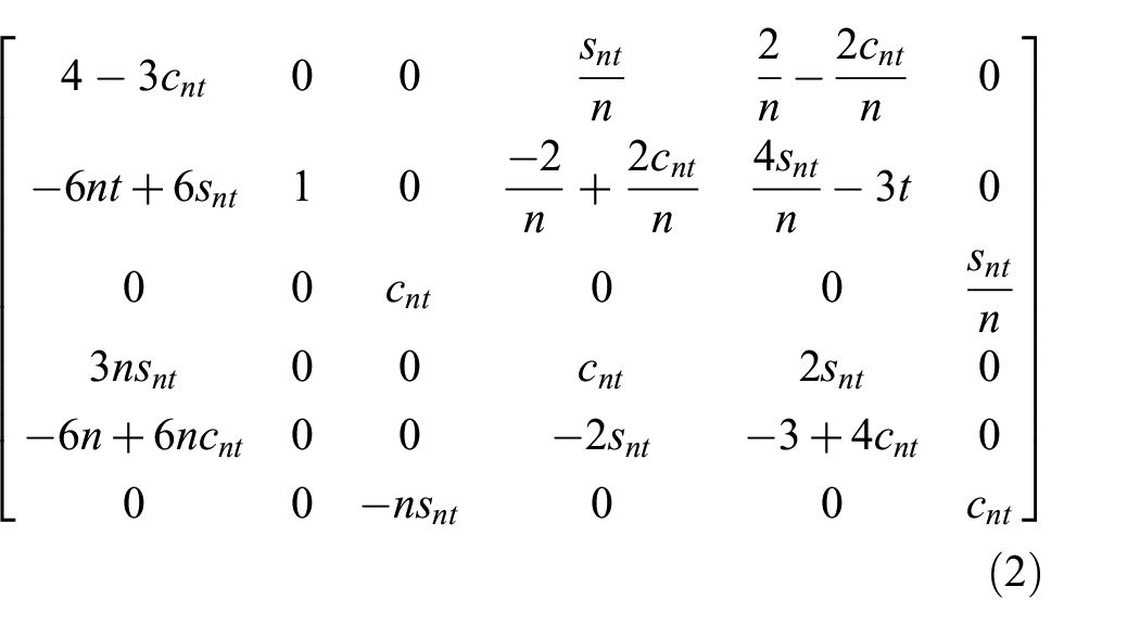
The corresponding state transition matrix, shown in Equation (2), is used to move forward each time step,
The frame of reference used is constructed as implied by these HCW equations of motion, with the origin in a geosynchronous circular orbit with radius
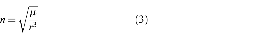
where
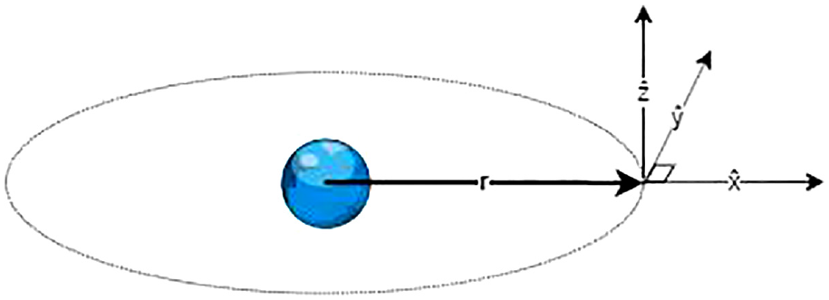
The local vertical, local horizontal (LVLH) frame. 4
A simple method for representing the angle of the sun is used in the simulation environment. The sun is considered to have an azimuth—the angle from the x-z plane in the counter-clockwise direction—and an elevation—the angle above the x-y plane. The azimuth angle can start anywhere on a full circle and moves in the negative direction at a rate of 360° per 24 h. The elevation can be initialized between
The simulation environment is stepped forward 60 s each step, for 720 steps which equates to 12 h. The simulation does not continue past 720 steps, but may also be stopped early if an agent exceeds the simulated sensor distance of 400 km from the target. These values were chosen to allow fast simulation times with a reasonable granularity of control available to the agent at the relative distances in the scenarios. The initial states and thrust magnitudes available to the agents were bounded to maintain realistic accuracy in HCW dynamics–all objects in the LVLH frame should be much closer to the frame origin than the orbit radius r.
3.2. Triangulation method
A realistic method for sensor noise generation and triangulation is proposed. The method for both should be not only reasonably realistic but also computationally efficient to allow for fast computation over potentially millions of simulation steps during training. Without sensor error, the triangulation accuracy may become so trivial that proper positioning of agents in the environment may not show improvement and encourage learning; however, realistic noise generation is computationally expensive.
To greatly reduce computation time during training, the standard deviation of angular noise is generated through simulation before training takes place and used to generate a lookup table. The lookup table is based on specifications from a chosen optical sensor with detection calculations using the method discussed by Kirk and Cain.
28
In short, the target is modeled as a 1-m sphere and is simulated at distances between 1 and 400 km in steps of 1 km,
where
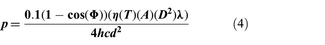
Missed observations and hidden information are beyond the scope of this work, but the probability of detection should be factored into the noise calculation. To take this into account, the sensors are assumed to report at the rate of the commercial star tracker, 10 Hz, and the standard deviation of the noise is altered by the probability of detection so as to mimic a filter. Since the simulation steps are set to 60 s and the rate is 10 Hz, the standard deviation of the noise is scaled by dividing by a factor of

and
The optical sensor specifications used for the majority of experiments in this work match that of a commercially available star tracker that might be used on a small satellite. This sensor is also compared to a much more powerful star tracker that may be found on a large satellite, and also to that of a camera similar to one found on a cell phone. A star tracker is not specifically required to be the sensor, and any optical sensor that could reasonably be used for target detection and LOS angle determination may be used. A sensor must be chosen that has performance characteristics fit for the distances in the simulation.
The three-dimensional (3D) position of an object can be determined by multiple (at least two) observations of it from star tracking cameras that report the direction the object is to them in an Earth-centered coordinate system. In this case, the star trackers will use the right ascension and declination of the object to provide a vector that points from the star tracker to the object of interest. It is assumed that the star tracker’s exact position is known in the Earth-centered coordinate system and this analysis does not factor in any uncertainty in the observer’s position into the determination of the object‘s position. The right ascension and declination angles are converted into a unit vector,
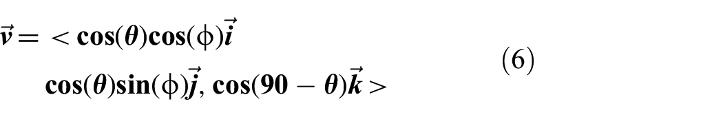
In these equations,

In this equation,

In this equation,
A second plane that intersects the one shown in Equation (8) is generated by taking the cross product between

The second plane is then computed as shown below:
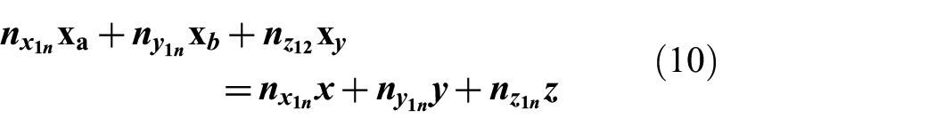
This process is repeated to obtain the equations for the intersecting planes that describe the line between the second agent and the object by switching the roles of the first and second agents in Equations (7)–(10). Every combination of agents making observations will therefore contribute four equations of planes that are involved in the solution for triangulating the position of the object.
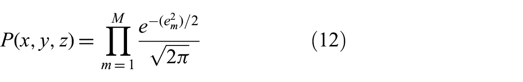
In order to derive a solution for the cartesian coordinates of the object that lies on all these planes, we define a Gaussian random variable,
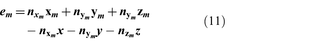
In this equation,
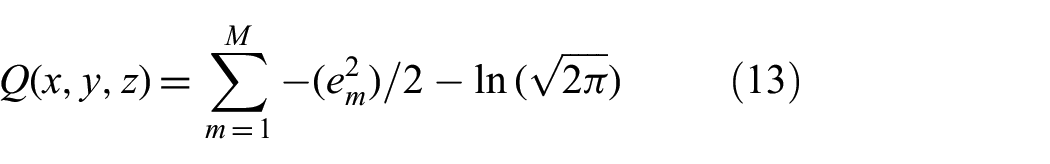
Taking the natural logarithm of P, the log-likelihood, Q, takes on the following form:
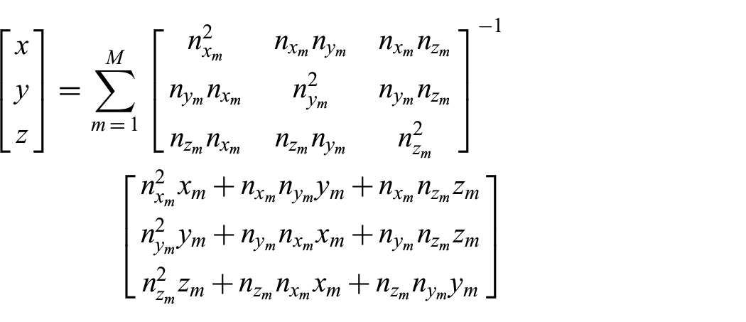
In order to solve for the (x, y, z) coordinate that maximizes Q, we differentiate Q with respect to x, y, and z set the results equal to zero and bring all the terms not dependent on (x, y, z) to the left side. This results in a system of equations:
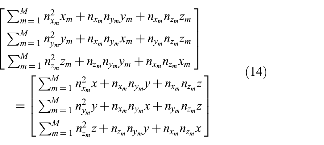
Factoring out (x, y, z) from this system reveals a matrix equation that can be inverted to solve for (x, y, z) with no pseudo-inverse required:
3.3. Observation and action spaces
What the agents can observe from the state and what actions the agents can take each step are important considerations. The agents are considered to have perfect information about their own state and the other partner agent states in the observation. The agents have more limited information about the state of the target but share this information between agents in their observations. This approach allows the policy trained to focus on the guidance portion of the GNC loop, and not over-fit to specific measurement errors that could potentially be handled by separate navigation and controller systems.
Observations given to the agents contain self position and velocity, position and velocity of each partner agent, and relative position and velocity to each partner agent in the LVLH frame. The agents also observe the angles of the sun as the unit LOS vectors to the sun. In addition, the agents also observe unit LOS vectors to the target in the same type of coordinate system as the sun angles vectors in the previous section, but do not know the range or any position or velocity information about the target. Each agent also knows this same information communicated from the other agents. The agents receive these angle readings even in operational conditions that would prevent the sensors from accurate readings and noise is not added to these observations, as learning to deal with missing information inputs is outside the scope of this work. Noise on the LOS angles is, however, considered for the triangulation accuracy objective, which is not observed directly by the agent when choosing actions.
The LVLH frame is recentered at the start of the episode. Though the target starts at the origin, the chief of the LVLH frame, the frame does not move or change during the simulation—the chief represents the origin of the frame only and does not move. All satellites, including both the agents and the target, are considered deputies in the LVLH frame.
The action space refers to the set of all possible actions the agent can take each step. The action space used for all scenarios in this work is a multi-discrete one—in each of the x, y, and z directions, the agent chooses to give positive, negative, or no thrust, implemented as an instantaneous change in velocity. Rather than continuous values for change in velocity or force, this greatly reduces the possible action set to only 27 choices. This potentially speeds up learning, but also allows mimicking bang-bang thrust control instead of only continuous thrusting. By abstracting the control to discrete changes in velocity, or delta-V, it allows the agent to focus on guidance and let control be handled by well-developed control theories for trajectory tracking 29 and prevents over-fitting to a specific type of controller. The discrete thrust for all scenarios is set to 0.1 m/s change in velocity in each direction.
It is assumed that the satellite is capable of adjusting attitude to make these changes in velocity and point sensors for observations. The satellite is assumed to perform impulse thrusts as requested once every 60-s step and would need to adjust attitude in that time. Attitude control is not part of the action space nor learned by the policy, so attitude is disregarded in these simulations to reduce complexity and computation time.
3.4. Scenario and reward strategy
The goal of the swarm policy is to minimize the mean error in the triangulation of the target position during a simulation episode. The environment space is likely too complex to have a policy learn to directly minimize this error while achieving good performance, so a reward scheme needs be created to encourage positioning that minimizes this triangulated position error of the target. Both the noise on the sensors detecting LOS angles to the target and computational accuracy of the triangulation method contribute to error in the triangulation accuracy. Based on the noise tables generated from the optics simulation sampling discussed in the “Triangulation method” section, the most important factor for sensor noise is sun illumination angle first, and distance from the target second. Intuitively, the triangulation method itself benefits from more agents contributing from unique LOS angles. The approach here is to use reward schemes meant to lead the policy into learning guidance decisions that would maximize the agents’ time in positions that would lower triangulation error.
In theory, a DRL agent can learn to perform complex tasks based on all or nothing rewards for success or failure, but in practice the idea of stumbling upon success from random actions in a highly complex environment is not reasonable in a finite time frame. Instead, the reward schemes developed may be used individually or stacked in layers that lead the agent toward good positioning. It is important to remember that the agent has no knowledge of these rewards during episodes, only the observations given. The rewards are only used later when updating the policy from batches of experiences, and only as summed values associated with observations and actions at each step. According to the PPO algorithm, 25 the policy will be updated to maximize future discounted reward.
First, a reward generator is created to encourage the agents to fly toward a desired state or relative distance. A common way to create this reward is as a reward field based on some function with respect to error or distance, such as a simple linear function,
14
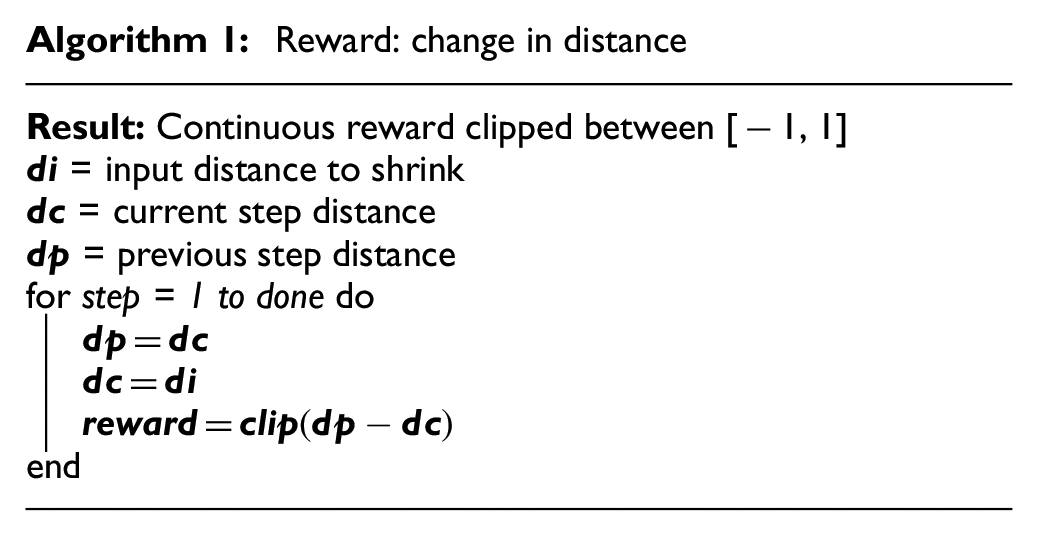
a logistic function, and normal distribution. Instead, here, a reward based on change of state is used to be more flexible and avoid the need for function parameters or coefficients to be tuned, similar to a reward used for RL aerospace baselines in the work by Ravaioli et al.
30
Algorithm 1 shows this proposed reward where, since the previous step, a positive reward is given if the agent moved closer to the desired state, or a negative reward if the agent moved away from the desired state. The magnitude of the reward is the distance changed, clipped between
Reward: change in distance
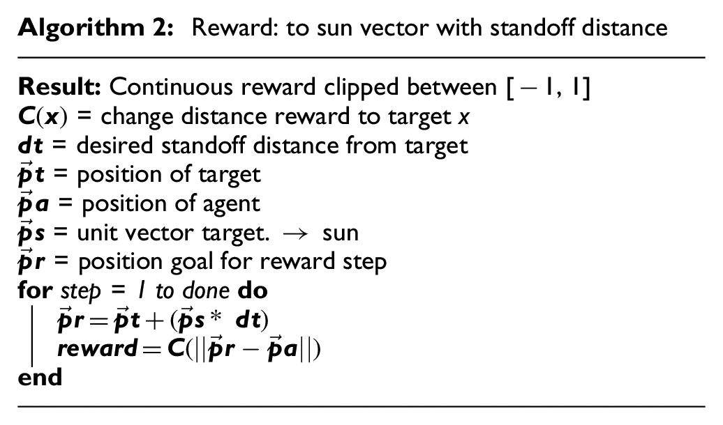
This change in distance reward can then be applied in multiple ways via choosing different desired end states. Since it is expected that angle to the sun is the most relevant environment factor for triangulation accuracy, two approaches are tested for encouraging learning that minimizes the error. First, the distance change is used to lead agents toward the vector from the target to the sun at a hold distance—this is a simple calculation from finding the unit vector of this direction vector and multiplying it by the desired standoff distance, as shown in Algorithm 2.
Reward: to sun vector with standoff distance
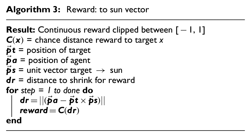
A second approach can also be formulated that removes the requirement for a hold distance by choosing the target distance to shrink to be the distance perpendicular to the sun vector from the target. If the sensor is accurate at all distances seen in the scenario, then this is a more direct approach. Since environment uses 3D points and direction vectors to represent the states, the most direct formula to calculate the distance
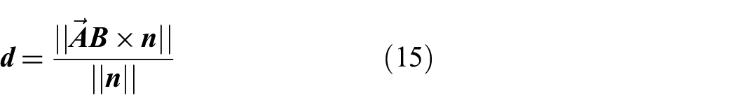
where
Reward: to sun vector
Other secondary rewards can be considered through simple calculations. In general, rewards should be scaled and/or clipped to be near the range of −1 to 1 and of similar order of magnitude to each other if used in combination. A reward for minimizing the triangulation error directly can be calculated by simply finding the distance between the true target location and the triangulated location and rewarding the negative of this value after clipping and scaling it appropriately—this will result in a reward that is negative, with a maximum value of zero for having no error. In addition, a reward is generated that is the probability of detection of the target, scaled and clipped, to encourage states where the sensor has the best performance.
Finally, a reward is created for encouraging fuel conservation. The is a scaled and clipped penalty of the delta-V used for a step’s action. The fuel used for this purpose is considered the two-norm of the absolute value of the action’s thrust vector. Care and tuning must be taken with this reward, as scaling too little will have no effect and scaling too high will result in the policy deciding that taking no actions would result in the highest overall reward.
Other rewards were experimented with but not included due to poor performance during exploratory trials. This includes using a linear reward based on current distance from the desired states instead of change in states, as well as a gaussian curve–based reward—these performed worse than the change-based function in Algorithm 1 while also requiring additional parameter tuning.
In addition, a reward encouraging the agents to spread out their LOS angles to the target was tested. This reward was a scaled and clipped value from the mean angle between the agent LOS vector to target and each other agents’ LOS vector to target—after extensive tuning attempts, the reward only confused and reduced consistency in training. Success for this type of reward would likely require prior knowledge of the most effective spread of look angles for triangulation with a particular sensor.
The rewards detailed here are tested individually and in various combinations to encourage the policy to learn minimizing triangulation error.
3.5. Training scenarios
Training will take place over thousands of episodes in parallel workers that are then used to update the policy in batches. The environment physics are deterministic, in that there is no random noise added to the states (except in the triangulation calculation as previously detailed), but the number of possible state combination for the target, agents, and sun in the continuous space is vast. Even with the vast number of available states, introducing random differences between episode starting states is important to avoid the policy over-fitting to perform sequences of actions that do not equate to learning the task itself. For an analogy, learning to walk down one specific hallway by repeating a sequence of steps with eyes closed is not desired, if the task is to learn to walk down any arbitrary hallway.
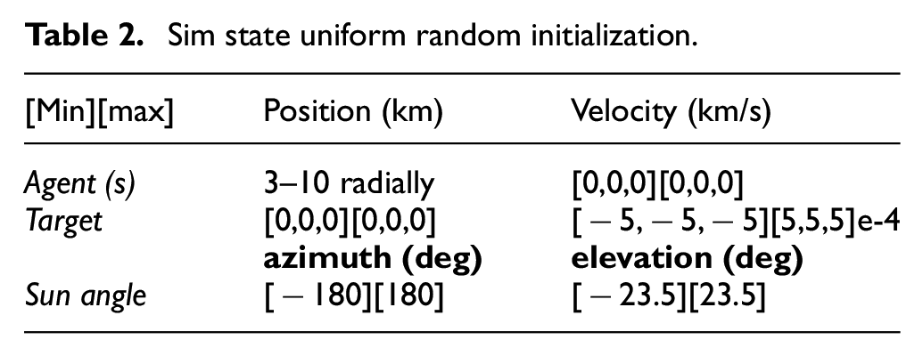
At first, an initial training run is performed without randomization to check the tasks with given starting magnitudes is possible to complete. After this validation, the agents, target, and sun are initialized randomly using uniform random variable samples in the ranges shown in Table 2. For special consideration, the agents are initialized spherically with a radial direction from the origin that is uniform random, and a uniform random distance that is between a minimum and maximum—this is to avoid instances where agents start on top of the target.
Sim state uniform random initialization.
With this state initialization, the policy will experience a vast range of possible states, forcing it to learn to complete the task based on observations and not by repeating a sequence of actions. Each agent in the simulation is set to use the same policy, and several policies will be trained separately with varying numbers of partner agents in the policy, and varying combinations of reward shaping. Intuitively, since at least two agents are required for the triangulation, increasing the number of agents in the simulation should increase the score. Since the lookup tables for the sensor data extend only to 400 km, episodes are stopped as “done” if any agent exceeds this range from the target.
Several policies with four agents and different combinations of reward shaping are trained on a local workstation to roughly measure the strongest combination with default training parameters. The best policy from these exploratory training runs is then used for hyperparameter tuning.
3.6. Hyperparameter tuning
After initial training runs are conducted across broad combinations of reward shaping, a training setup of four agents with the reward from Algorithm 2, a triangulation error reward, and probability of detection-based reward are chosen. A hyperparameter sweep is conducted in two phases.
The first phase consisted of a broad search over seven parameters with 200 samples. A computer cluster is used with Ray Tune for the search, with 70 cpu threads available; these are split among seven workers, each utilizing nine cores for gathering experience and one for a driver (seven simultaneous samples). The scheduler used is RLlib’s asynchronous hyperband, maximizing reward over up to 2000 iterations, with a patience of 200 iterations. The parameters searched over in the first phase were learning rate, clip param, lambda, Kakade and Langford (KL) coefficient, number of epochs, batch size, and mini batch size. All ranges and sample functions were set according to the best practices in the Ray documentation. Some parameters were found to be less productive for tuning, and the scheduler settings too passive for patience that led to long computation time (over 2 weeks). In addition, the reward was found to be not fully linearly related to the primary metric of mean triangulation error.
To adjust for these issues, a second phase of tuning was conducted over a tighter search area. The scheduler was set to minimize mean triangulation error instead of maximize reward, with only 1000 iterations max and 100 iteration patience. In addition, entropy coefficient was added to the search parameters. The parameters searched over in both phases, along with their ranges and sampling functions, are shown in Table 3. This second phase with new parameters was more productive with a completion time of 2 days using 150 CPUs total (15 simultaneous samples).
Parameters for hyperparameter sweeps.

After a policy is trained in randomly initialized environment scenarios with the best combination of training hyperparameters chosen, it is prudent to develop specific controlled scenarios for evaluation, as discussed in the next section.
3.7. Model evaluation strategy
Rather than maximizing reward, the models are evaluated on the metric of minimizing average triangulation error. The scenarios studied here are not based on any real mission needs, so there is no end goal for performance. The only goal is to train policies that can learn to improve on the triangulation accuracy.
Multiple policies are trained from fresh starts with the configurations described in the previous section, changing the reward shaping used or the number of agents in the training run from a minimum of two agents, successively to a maximum of five agents. Training results from each run are compared to observe how increasing the number of agents affects performance. A policy with good performance is then chosen and used in specifically controlled evaluation scenarios to observe how the policy handles different scenarios.
The scenarios start with initial states that should intuitively be easy starting states, and also tested at difficult starting states such as bad distance and sun angles. The policies are also evaluated at starting states that are beyond the ranges seen during training, and a scenario where the target maneuvers during the middle of the episode (during training, the target only maneuvers at the first step).
Since the policy controls agents individually, in theory, the number of satellites used could be increased arbitrarily in implementation/evaluation; however, since the policy is tied to the observation space as implemented in RLlib, a mismatch of agent number between training and evaluation is not tested here. This would require developing a more complex observation space function and left for future work.
4. Simulation results
The results are presented in this section in five parts: the parameters chosen as best from the hyperparameter searches, the training results for different combinations of reward shaping and varying numbers of agents in the swarm, a comparison of optical sensors in the environment, fuel conservation results, and evaluation trials for the best policies.
4.1. Hyperparameter search results
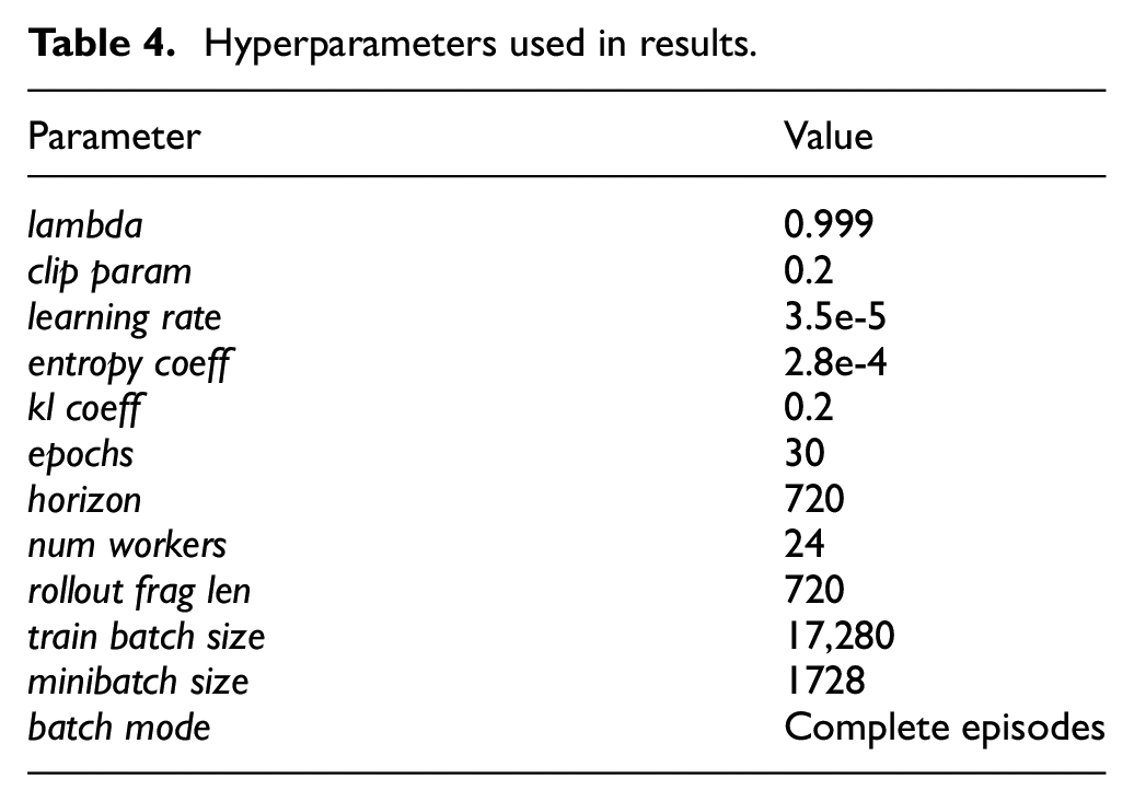
After two phases of hyperparameter sweeps, four parameters were found to be the most productive for tuning: learning rate, lambda, entropy coefficient, and clip parameter. These parameters had the most effect on training outcomes for minimizing the error metric.
The parameters for training batch size and minibatch size were found to be less productive to tune, so long as the former was large enough for gathering experience and the latter was around 10 to 20 times larger. The horizon parameter was set to the length of the simulation episodes, and the rollout fragment length set to this horizon so that whole episodes are included in training batches. With these ratios in mind, the training batch size used was the rollout fragment length multiplied by the number of workers, and the minibatch size 10 times less than this training batch size.
The KL coefficient and number of epochs were found to be best at the RLlib default parameters. The full parameters used in these results are detailed in Table 4. All other parameters not mentioned were left at the defaults in RLlib 1.13.0.
Hyperparameters used in results.
4.2. Training results
It is useful to analyze both the metrics over the course of training and evaluate performance of a trained policy in specific scenarios. The training metrics of training runs are analyzed—first for different reward shaping techniques discussed in, and second for different numbers of agents cooperating in the simulation. Then, a series of specific evaluation scenarios are run with a chosen policy. The scenarios are designed to encompass both easy and difficult examples and include both scenarios that would be commonly experienced during training and scenarios that could not have occurred during training. Testing response to starting positions and events not seen during training explores the ability for the policy to generalize beyond the training experience. It is important to recall that each agent in a scenario makes independent decisions based on a single policy, but the policy acts for a single agent and does not act as an overlord controlling all agents at once. Each agent is an individual in the swarm.
The figures in this section show the learning over time while training the policy. The metric is the mean distance error of triangulation calculations in an episode, and this mean is averaged across episodes and displayed in the graphs as the error per total training experience in steps.
Figure 2 shows how different reward shaping affects the metric of triangulation accuracy during training, with each policy shown using four agents in the episodes. Using triangulation error as the only reward (“Error Only”) results in very slow learning that never breaks past an error lower than 1 km. Though performance does improve over the initial random actions, directly seeking to minimize the error is a nebulous task that does not encourage the best learning. The best training results came from the reward shaping in Algorithm 2, the distance reward for flying toward the target’s sun vector while trying to maintain a distance from the target of 5 km (“Sun Vec 5k”). The reward in Algorithm 3 that rewards moving directly toward the target’s sun vector without consideration for distance from the target does not perform as well (“Sun Vec”), achieving only around 100 m average error as opposed to 10 m average error in the previous reward. The rewards in the legend of Figure 2 refer to the following:
Sun Vec: Algorithm 3 reward only, returning a change of distance-based reward for moving closer to the target’s sun vector with no consideration for distance from the target.
Sun Vec 5k: Algorithm 2 reward only, returning a change of distance-based reward for moving closer to the point on the target’s sun vector that is also 5 km away from the target.
Error Only: Only rewarding the agent the triangulation error distance, scaled and clipped.
3 Rewards: Rewarding the agent with the reward Sun Vec 5k above, as well as the Error reward above, and third a scaled and clipped value of the probability of detection for that agent’s sensor to detect the target each reading.
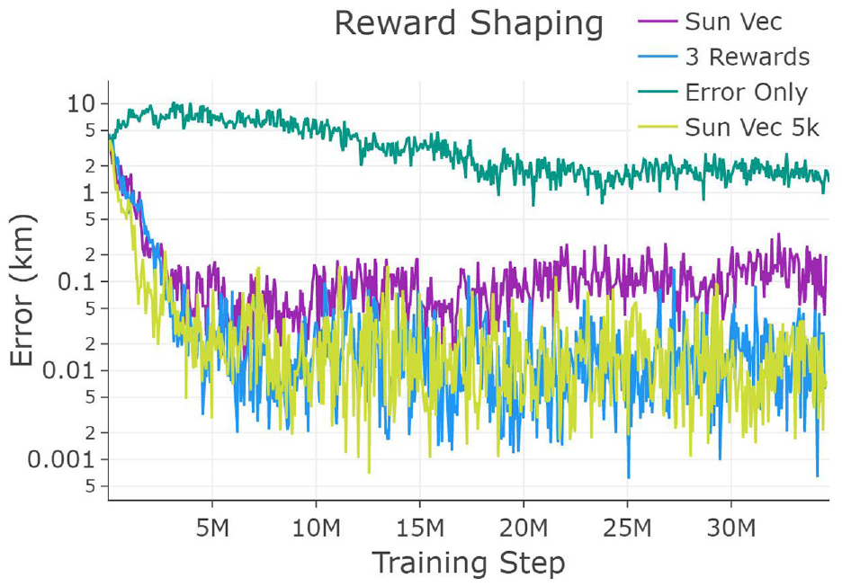
Error over training iterations, per reward shaping used. Rewarding based on error only gives the worst error results (top), reward “Sun Vec” gives the second from the top result that is a significant improvement, and the two best (“Sun Vec 5k” and “3 Rewards”) are overlapping within each other’s noise as the lowest error. All training runs here use a the small star tracker sensor and four agents.
Adding additional secondary rewards for the triangulation error and probability of detection does not have as significant of an effect on the mean error in the best policies; however, after many training experiments, these rewards add a small level of consistency between experiments, so long as the secondary rewards have been tuned to be in the same order of magnitude as the primary reward. A reward for encouraging the agents to spread out their look angles was also trialed but did not improve the error metric, and in fact led to less consistent training results and therefore its use was not continued.
Overall, the policies with the best reward shaping quickly learn to cut the average triangulation error by nearly three orders of magnitude compared to the initial iterations which only take random actions. Using four agents in the simulation fits well for this experiment for balancing low error and fast training time, and the middle-powered sensor fit for a small satellite allows a large opportunity for growth through learning while not making the task too difficult at the ranges in the simulation environment.
In addition, different numbers of agents were used in training runs to compare how higher numbers of agents affect performance, from the minimum of two agents and up to five agents. Each policy trained in this case uses the “3 Rewards” reward shaping in Figure 2. With a well-tuned training setup for hyperparameters and reward shaping, the number of agents in the swarm does not play a significant factor at these ranges with this sensor. The policy with only two agents ends with a mean training error of 0.5 km, while the policies with three, four, or five agents end with mean training error around 0.2 km. This can only be estimated with heavy smoothing of the data due to being within the level of noise seen during training. For consistency the policies will default to using four agents in other evaluations. The measurable difference between numbers of agents in the sim is more significant when the policies are not well tuned, and also would likely become more significant in environments where sensor power is more critical.
Figure 3 shows how different quality levels of optical sensors used in the simulation affect performance. The “Small Star Tracker” refers to data based on a commercially available star tracker that may fit on a small satellite such as a CubeSat. The “Large Star Tracker” refers to data based on a test bench high-performance star tracker that would unlikely be used in this application due to size, weight, and cost. The “Cellphone Camera” refers to a sensor based on a modern smartphone camera. The sensor does not need to be used for star tracking but need only be able to return relative angle information to a target on detection. The same sensing rate of 10 Hz was assumed for all sensors.
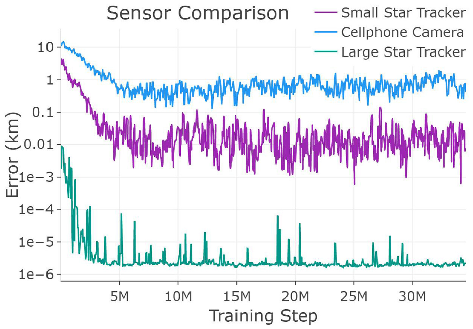
Error over training iterations, per power of optics used. Top: cellphone camera, middle: small star tracker, bottom: large star tracker from highest to lowest error. All training runs here use the “3 Rewards” reward shaping and four agents.
The middle performance sensor was used for all other results in this research, giving a balance that is intended to allow the most growth in accuracy from the policies learning the task. The large sensor also allows for growth but quickly bottoms out the error by achieving near millimeter accuracy. Conversely, the cell phone sensor proves too challenging to achieve a desirable accuracy at these distances but may be improved in future work with higher levels of agent number scaling in the swarm.
Finally, the reward shaping setup with three rewards and four agents was trained with an additional reward for fuel. This reward was simply a punishment per fuel action, requiring tuning to find the correct value for punishment. Figure 4 shows the fuel use over the course of training comparing the overall best policy (using the 3 Rewards combination and four agents) versus the same training setup with the fuel reward added and tuned. Based on the thrust available to the agent, the best value for the punishment was found to be 3500 per delta-V used per step. Values significantly lower than this had no effect on fuel conservation, and values significantly higher than this led to the policy choosing to take no actions in order to maximize the total reward. The fuel conversation policy had no noticeable performance loss during training while using two-thirds less fuel.
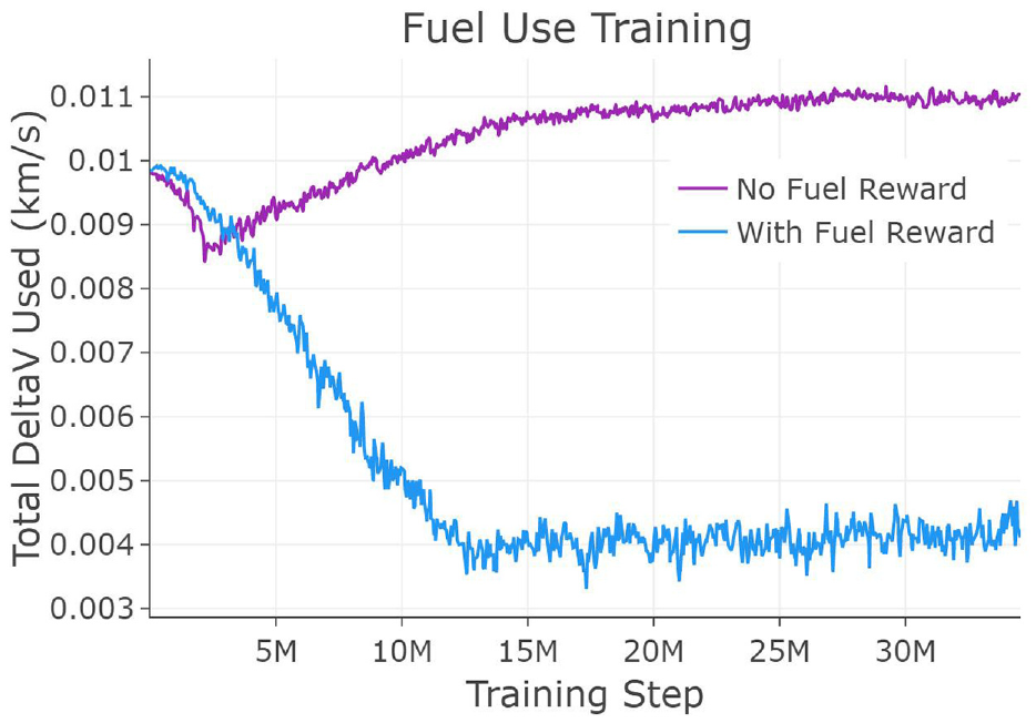
Fuel use per episode comparison. Average fuel used by one agent in an episode, trained with four agents using the “3 Rewards” reward shaping and the small star tracker sensor. The top line corresponds with no fuel reward, while the bottom line, nearly threefold lower fuel use, corresponds to the policy with fuel reward.
Overall, the training results show that policies are able to be learned that significantly improve the triangulation accuracy over random actions from the start, cutting the error around three orders of magnitude.
4.3. Evaluation results
In addition, while analyzing performance over training, it is important for DRL experiments to evaluate trained policies in specific scenarios. In this section, eight evaluation scenarios are discussed that seek to cover a wide range of scenarios of varying difficulty. Some of the evaluation scenarios are purposely set as edge cases or even situations that could not have been experienced during training, so as to stress the ability of the policies to generalize.
For each evaluation scenario, the sun starts at 0° in azimuth and elevation for consistency in comparison. The target always starts at the origin as in training but has the same initial velocity (akin to a maneuver at the start of the episode) unless otherwise stated. Due to the nature of DRL, the policy does not make the exact same choices each episode, even if the randomization of the starting states is removed; therefore, each evaluation scenario is repeated for 2000 episodes and evaluated based on the mean and deviation across the total episodes. The best policy for the 3-reward setup is used for evaluation as described in 3 at its final training state (labeled “base”) and compared to the equivalent policy that is trained with the addition of fuel-saving rewards (labeled “fuel”). Table 5 details the starting positions of the four agents in each scenario, along with the mean error across all 2000 episodes for these two policies. Table 6 shows more detailed statistics for each scenario, including the standard deviation of the triangulation error and the 80th, 90th, 95th, and 99th percentiles for the error to measure the consistency and presence of outliers. The intent of each scenario is as follows:
Basic formation surrounding the target at the max starting distance used in training;
Worst case for LOS angle separation, with all agents starting at the same point at max training distance;
Shortly outside staring distance seen in training, but with good LOS separation;
Surrounding formation with starting distances double the max training distance;
Surrounding formation in ideal starting distance for the primary reward shaping
Surrounding formation at max training distance but the target remains stationary at the origin;
Surrounding formation in ideal starting distance but the target remains stationary at the origin;
Surrounding formation in ideal starting distance, but the target unexpectedly maneuvers sharply at the 360th sim step.
Evaluation scenario results with mean triangulation error in 2000 episodes, using the best policy with 3 Rewards reward shaping elements and no fuel-saving training (base error) and the same design with added fuel-saving reward during training (fuel error).
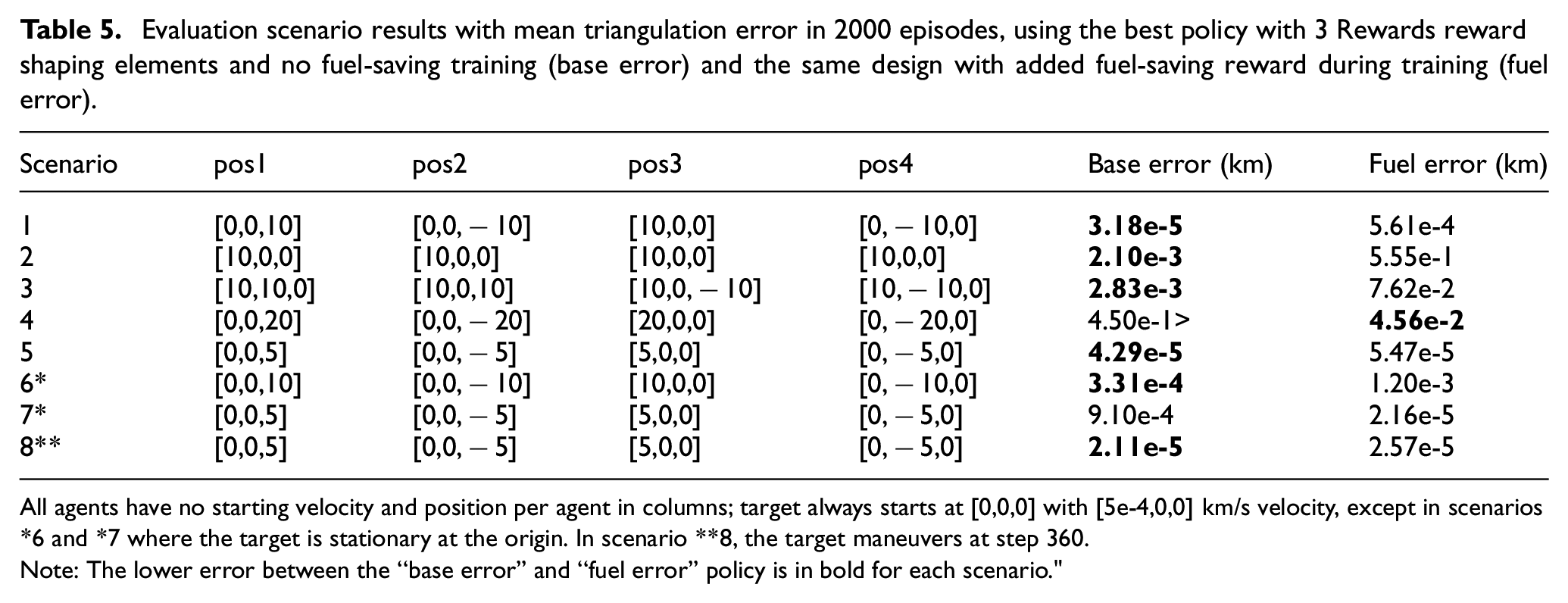
All agents have no starting velocity and position per agent in columns; target always starts at [0,0,0] with [5e-4,0,0] km/s velocity, except in scenarios *6 and *7 where the target is stationary at the origin. In scenario **8, the target maneuvers at step 360.
Note: The lower error between the “base error” and “fuel error” policy is in bold for each scenario."
Statistics comparing the policy without fuel conservation (base) and with (fuel) across the eight evaluation scenarios, including the mean, standard deviation, and 80th, 90th, 95th, and 99th percentile errors.
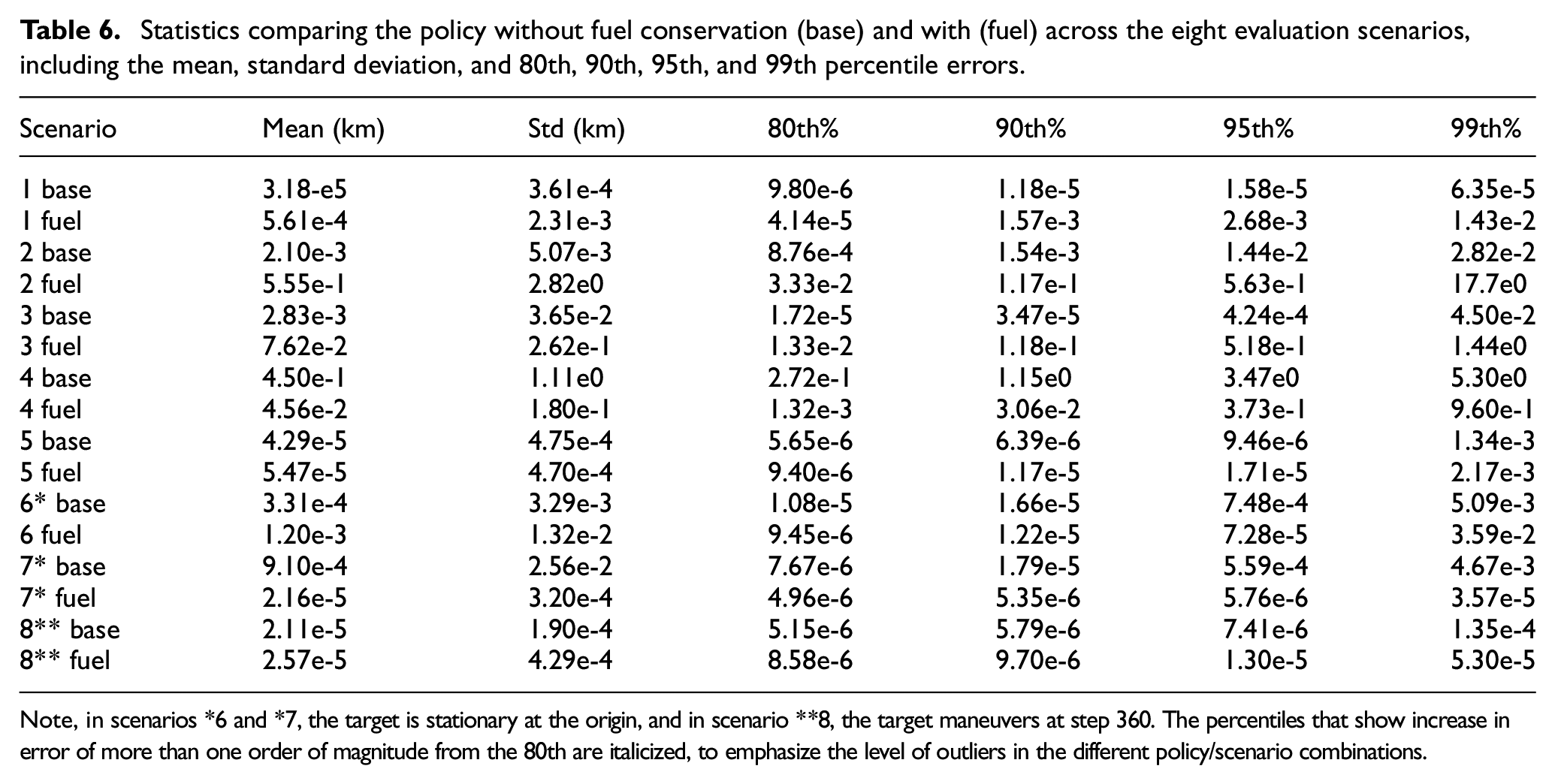
Note, in scenarios *6 and *7, the target is stationary at the origin, and in scenario **8, the target maneuvers at step 360. The percentiles that show increase in error of more than one order of magnitude from the 80th are italicized, to emphasize the level of outliers in the different policy/scenario combinations.
The base policy achieves very high accuracy across most of the evaluation scenarios, with mean error on the order of centimeters. The general strategy of the policy appears to be following the target at a distance of 5 km while using varying corkscrew-like trajectories to achieve advantageous and varying sun and LOS angles. The fuel-saving policy has smoother trajectories, as the punishment for actions acts like a dampening effect.
The most significant challenge, and the worst error, comes from scenarios where the starting distance of the agents are far from the target or when starting with LOS angles to the target that are poorly spread out between agents. Interestingly, the fuel-saving policy manages to significantly outperform the base policy in the very high distant case, as well as the case where distance is ideal but the target is unexpectedly not moving. During the extreme range case, the more aggressive corkscrewing of the base policy works against it, when a more direct path toward the target to close distance would be better.
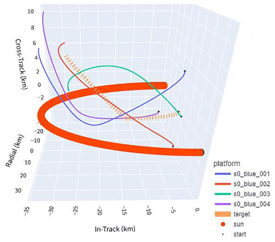
An example of scenario 2 from the base policy reveals that the secondary reward for minimizing the error directly influences the maneuvers, causing the agents to vary their trajectories even when the primary reward shaping would seek to maximize individual positioning. Figure 5 shows an example of a well-performing run in this scenario, notably showing the agents varying their trajectories. This varying of trajectories remains consistent across evaluation episodes. The fuel-saving policy struggles much more with this particular scenario, with mean error two magnitudes worse, suggesting that maximizing thrust is important to achieve high accuracy in this edge case. The agent satellites appear to struggle to find reachable trajectories that both achieve distance and sun angle goals, while also spreading out enough to have varying LOS angles to the target.
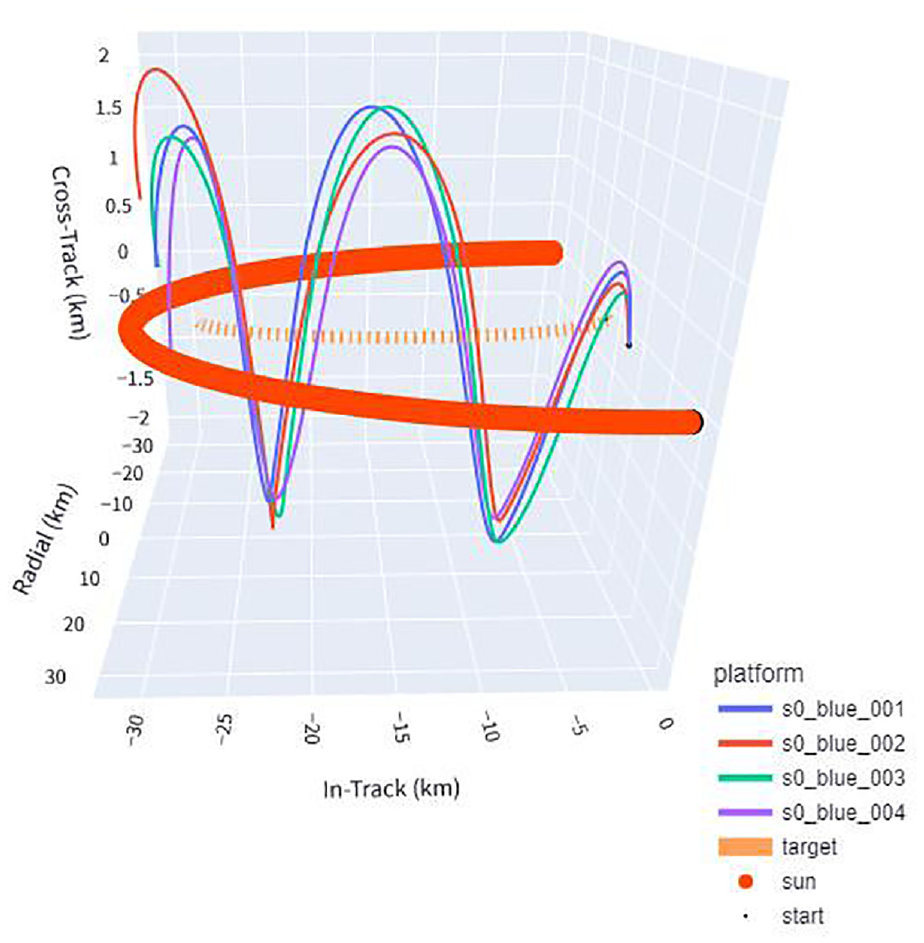
3D example of evaluation scenario 2 (agents start at same point), base policy. All agents start at the same point, and notably are seen to spread themselves out instead of taking the same path, even though that was not specifically rewarded. The dashed line represents the target, the thick line the angle of the sun, and the rest the flight paths of agents.
Scenarios 6 and 7 differ from the preceding scenarios in that the target remains completely stationary at the origin—a state that is unlikely to be seen during training. The base policy suffers a small hit to accuracy in these scenarios, likely due to the strategy it seems to have learned—reviewing the spread of actions and fuel use during episodes shows reveals the policy maximizing the use of thrust to minimize the error, using trajectories that seem aggressive and erratic to intuition. This strategy is less advantageous when the target is unexpectedly not moving, and Figure 6 shows this behavior.
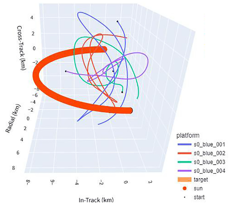
3D example of evaluation scenario 7 (stationary target), base policy. The policy here, without fuel conservation as a reward, chooses to thrust all the time even when the target is not moving—a state unlikely to be seen in training. The target remains stationary at the origin, the thick line represents the angle of the sun, and the other lines represent flight paths of agents.
The policy with fuel-saving behavior acts as a dampening mechanism to the control, giving it an advantage in the cases where less thrust is required, and more restraint on thruster use is desirable. Figure 7 shows how the fuel-saving policy differs compared to the base policy in Figure 6. Take special notice of the trajectory of the second agent this scenario with the fuel-saving policy. Consistently throughout the episodes, this agent choses to use the decoupled z axis in the HCW dynamics to thrust directly upward in an efficient manner; note that this is undesirable in a real scenario due to the collision course with the target, but the training scenarios in the scope of this research did not include collision avoidance. This behavior that emerges shows remarkable restraint on fuel use, as well as unexpected deviance from the usual strategy displayed—moving toward a 5k distance from the target between the target and sun, while following a corkscrew-like path. In this edge case scenario, the fuel-saving policy uses nearly 10 times less fuel than the base policy overall.
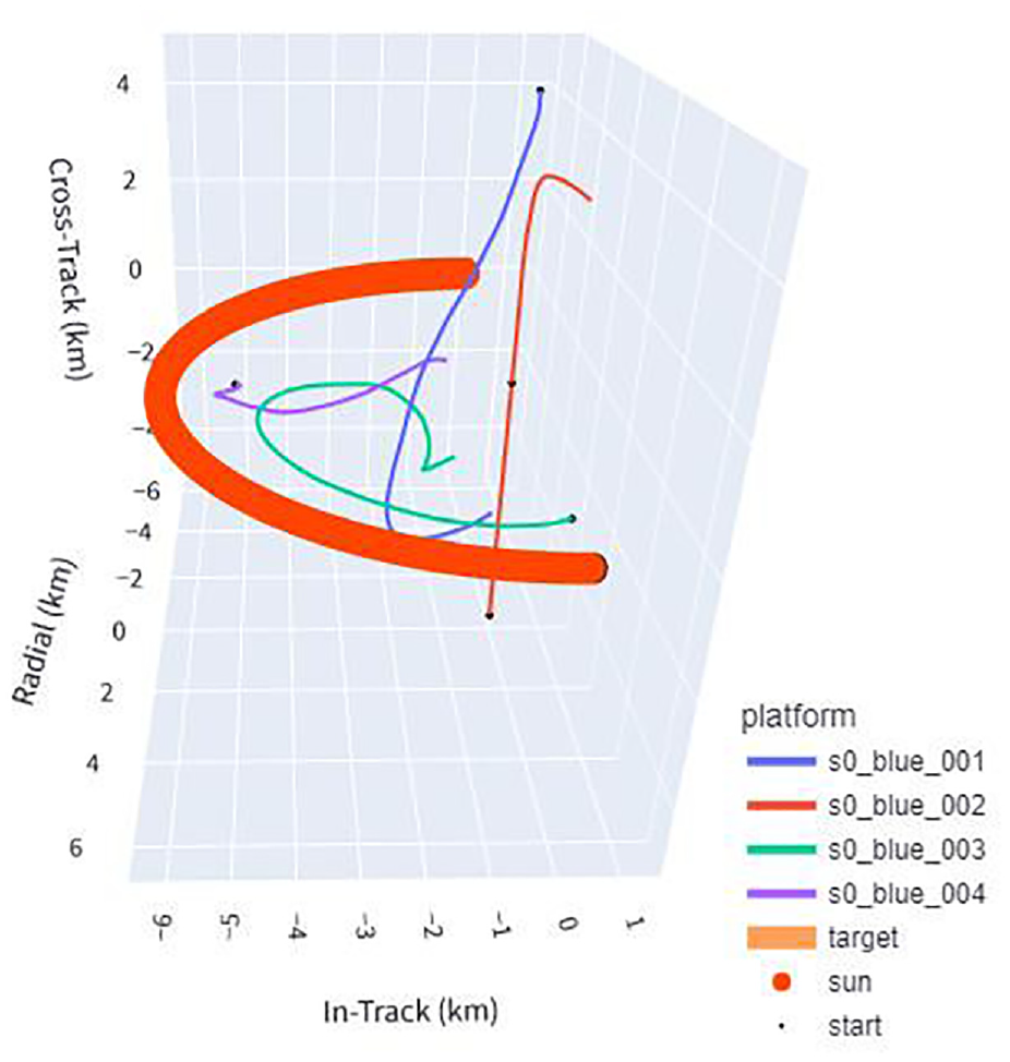
3D example of evaluation scenario 7 (stationary target), fuel-saving policy. The fuel-saving reward results in a very conservative approach compared to the policy in Figure 6. The second agent consistently takes advantage of the decoupled movement in the
Scenario 8 has the target maneuver halfway through the episode, which was never seen at all during training. During training, the target always maneuvered at the start and then followed a path based on that initial velocity. In this scenario, the target takes a sharp maneuver upward in the positive z direction. Despite the challenge of meeting an event that was never seen during training, both the base policy and the fuel-saving policy perform extremely well. In fact, this scenario has overall the lowest error of all training scenarios, likely due to the fact that the upward change in direction presents a slightly better sun angle for the agents than when the target remains in the x-y plane. The trajectories for the base policy and the fuel-saving policy are shown in Figures 8 and 9, respectively. These views best highlight the differences between the base and fuel-saving policies, with the corkscrewing effect present in most scenarios for the base policy and the dampening effect in the fuel-saving policy.
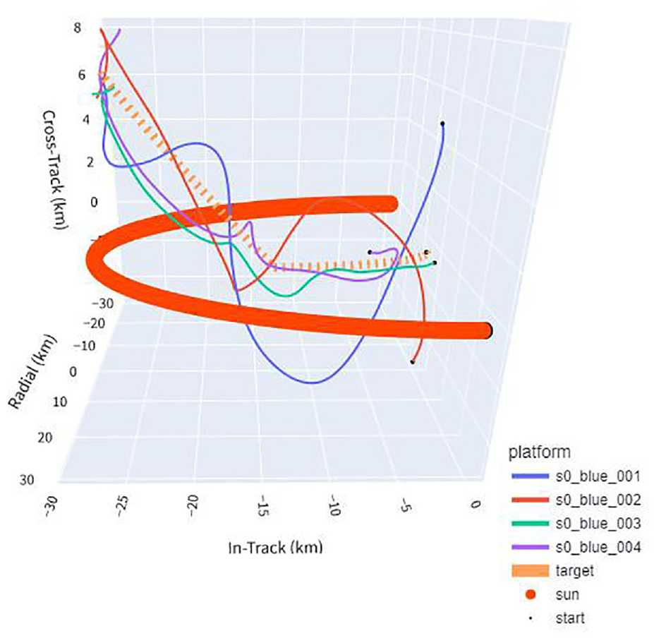
3D example of evaluation scenario 8, base policy. The target maneuvers upward halfway through the episode, which is never seen during training. Despite this, the policy uses aggressive, tight corkscrew movements that adjust to the maneuver and maintain high triangulation accuracy. The dashed line represents the target, the thick line the angle of the sun, and the rest the flight paths of agents.
3D example of evaluation scenario 8, fuel-saving policy. The target maneuvers upward halfway through the episode, which is never seen during training. Despite this, the fuel-saving policy maintains high triangulation accuracy by gently adjusting trajectory while maintaining distance from target and sun angle. The dashed line represents the target, the thick line the angle of the sun, and the rest the flight paths of agents.
Regarding consistency and outliers, it can be seen from Table 6 in the percentiles that the policies have high consistency and few outliers outside of the scenarios that are meant to be the most challenging examples. Both policies achieve meter-level mean accuracy or better in most scenarios up to the 95th percentile, and in some scenarios even at the 99th percentile. From reviewing a wide range of episodes across different performance levels, performance outliers that achieve tens or hundreds of meters error are usually caused by small mistakes in trajectory, such as the agent appearing to aim for curving around behind the target but instead passing in front of the target. The observations passed to the agents are angles-only and have no explicit range or position information about the target. Range and position to the target can only be inferred by the combined angle observations of multiple agents being shared in the observations. Given the difficulty of this, the policies are remarkably consistent. The most challenging scenarios contain outliers that reach the kilometer-level error, and these extreme outliers are seen when multiple agents lose a sense of distance to the target and fly far away. These cases are rare outside of scenario 4, where the agents start at a range from the target that is double the max starting range seen during training.
5. Conclusion and future work
During this initial investigation to cooperative swarming, the DRL agents were found to be able to learn guidance tasks that seek to maximize average accuracy in triangulating a target that is moving in the relative frame after maneuvering. This highlights a distinct and flexible approach that may prove advantageous to more traditional GNC such as multi-hypothesis tracking, model-predictive control, dynamic programming, greedy heuristics, or others. The task for multiple agents to maneuver for high-accuracy triangulation of a moving target was chosen as an arbitrary but challenging task for a swarm, and is comparable to other proximity operations of interest such as on-orbit inspection and servicing tasks, but with a more concrete performance metric.
Training policies with varying numbers of swarm agents and different approaches to reward shaping showed results that conclude the ability of DRL policies to improve on the goal metric of a complex task in realistic on-orbit simulation. The policies learned to improve from kilometer-level mean error in the triangulation with random actions, to centimeter-level error in average evaluation scenarios. The policies were able to adjust to many edge cases that would rarely, if at all, be experienced during training, and even perform well in cases that were never seen during training such as additional maneuvers from the target.
In addition, implementing fuel-saving reward shaping was shown effective, lowering fuel use by two-thirds, with minimal impact on performance in most cases. The fuel-saving policy served to also dampen the system, proving advantageous in certain scenarios and behavior that may be more desirable depending on potential user needs.
Different power levels of optics were also explored and compared, which may give insight to hardware needs for similar scenarios at this orbit regime and distances between spacecraft. Future work includes further exploration methods for performance with low-powered sensors that might be used on very small satellites in large numbers—a highly scalable swarm.
To achieve greater levels of scaling and flexibility, future work also includes decoupling the number of agents in the swarm from the DRL model. Though the policies control each agent individually and with the same strategy, the observation spaces couple the number of partner agents to the policy in this research. This in turn makes the number of agents fixed to the policy once trained and is not ideal for flexibility in the concept of a swarm. Future work will decouple the agents from the observation space to allow the swarm to scale to any number of available platforms.
Overall, the work herein represents an important initial step to improved autonomy in on-orbit proximity operations.
Footnotes
Funding
The author(s) disclosed receipt of the following financial support for the research, authorship, and/or publication of this article: The authors received financial support for the research in this article from the Air Force Research Laboratory, Space Vehicles Directorate, Kirtland AFB, NM, USA.