Stochastic attrition modeling

1. Introduction

Lanchester’s theory of combat has provided military analysts with a means of quantifying attrition between two equally equipped fighting forces. In the work by Lanchester, ¹ there was subsequent development of Lanchester’s fundamental work to reflect evolutions in ground-based combat operations.^2–4 Interest in Lanchester’s equations, as well as modifications of them to reflect changes in warfighting, has continued to be reported in the literature. The application of these equations to real combat operations has been examined by Turkes ⁵ and Lucas and Turkas. ⁶ The extension of the models to a three-dimensional setting has been investigated by Spradlin and Spradlin ⁷ while Kress ⁸ provides a formulation for analysis of irregular warfare. Along similar lines, Markowsky and Markowski ⁹ explore Lanchester’s equations to model cyber warfare. Extension to utilizing partial differential equations for combat modeling has also been considered.^10,11

Addressing more contemporary issues ¹² considers the application of Lanchester’s equations for attrition modeling in the current Russian–Ukrainian conflict. Biologists have also examined the application of Lanchester’s equations to study combat in ant populations ¹³ as well as conflicts between social animal groups. ¹⁴ Hence, the study of attrition modeling, and in particular analysis via Lanchester’s equations, continues to be of relevance in contemporary studies of warfighting.^15–18

Recall that Lanchester’s square law equations stipulate attrition of two fighting forces in terms of the two differential equations

where B ( t ) and R ( t ) are the sizes of BLUFOR and REDFOR combat teams at time t , respectively. Each of the equations in Equation (1) implies that the casualty rate between the two similar fighting forces is proportional to the number of combatants in the opposite force at time t . The parameters and β correspond to offensive firepower levels of REDFOR and BLUFOR, respectively.

Stochastic variations of Lanchester’s equations have also been considered. The two main approaches have involved either modeling the number of combatants still alive through Markovian processes or introducing stochastic differential equation variants of Equation (1) to model uncertainty.^19,20

The novelty in this study is to examine the fundamental problem of attrition between two comparable fighting forces by introducing a stochastic lifetime analysis. It will be assumed that each individual in BLUFOR has a lifetime specified through a conditional distribution. The latter is designed to replicate the primary assumption in Equation (1) that a combat team’s size will vary by a constant multiple of the size of the enemy force at time t . Based upon some validated results in the literature, a particular model will be applied for this conditional distribution. In addition to this, REDFOR arrivals into the theater of operation will be modeled by a stochastic process also based upon results from analysis of actual attrition modeling. The analysis of BLUFOR team survivability will be undertaken through considerations of lifetime order statistics. Specifically, the statistical event that an order statistic exceeds a given time will be shown to relate to BLUFOR possessing a specific number of combatants at the same given time. This then permits analysis of combat team survivability based upon investigations of order statistics. This is a considerable simplification on the alternative, which is to introduce a generalized binomial model to determine BLUFOR attrition.

Although the results will be focused predominantly on independently distributed lifetimes, it will be shown how correlated lifetimes can also be integrated into the analysis. Hence, the methodology in this paper provides a more general way in which to model combat attrition than is possible through Lanchester’s equations. In addition, the lifetime analysis approach may be adopted to the study of attrition in a number of contemporary operational environments, such as the analysis of swarms of drones.

It is also important to note that this study considers attrition of BLUFOR only; the analysis may be switched to apply from REDFOR’s perspective if required. The paper is organized as follows. The following section derives the lifetime model for combatants and outlines how order statistics may be used to measure attrition. A series of examples is then considered to show how the lifetime statistic approach may be used with given attrition and REDFOR arrival rates. These examples will show that the model provides a more general way in which to assess combat team survivability than is possible through Lanchester’s equations. The conclusions will indicate where further avenues of work are possible.

2. Mathematical model

The key idea in the following is to base attrition analysis on properties of a statistical model for an individual team member’s lifetime. Hence, it will be necessary to provide such a model that has been validated against real data. It is also necessary to determine a suitable model for REDFOR arrivals into the combat scenario. Some early studies have suggested the validity of renewal process models to account for combat attrition numbers, such as Karr ²¹ and Cho, ²² which provides a mathematical basis for the assumptions to be adopted. However, two studies of real attrition data provide direct validation of modeling assumptions.

An analysis of mortality rates in combat teams was examined by O’Donnell and Blood ²³ who considered US Marine Corps records for a 150-day period in the Korean War (1950–1953) as well as a 90-day period of the Okinawa operation (1945) during World War II. Statistical distributions were fitted to wounded in action (WIA), killed in action (KIA), and disease and non-battle injury (DNBI) measurements. Since the analysis in this paper is concerned with attrition due to direct engagement, the interest is in lifetime models for WIA and KIA cases only. The key result from O’Donnell and Blood ²³ was that a compound Poisson process could be used to model arrivals into the combat scenario (accounting for WIA and KIA statistics) where interarrival times of the process were exponentially distributed. Since interarrival times coincide with changes in the fighting force, it follows that the data analyzed by O’Donnell and Blood ²³ support the assumption that combatant lifetimes are exponentially distributed. Further validation for the modeling assumptions has been provided by Zouris et al. ²⁴ who also analyze casualty data for WIA and DNBI rates. This analysis has been based upon statistics obtained from four representative combat phases from Operation Iraqi Freedom (OIF) (Iraq, 2003–2011) and Operation Enduring Freedom (OEF) (Afghanistan, 2001–2014). This study supported the analysis by O’Donnell and Blood ²³ demonstrating that, for example, WIA casualty rates during a number of phases of OIF could also be modeled through an exponential distribution. However, it is important to note that Zouris et al. ²⁴ also show that two-parameter models, such as the Weibull and gamma, also fit WIA rates. This may be attributable to the fact that these distributions increase the number of modeling parameters to two, allowing for improved fit to real data. Model improvement through increasing degrees of freedom is a well-known phenomenon. ²⁵

Hence in this paper, it will be assumed that individual lifetimes will be exponentially distributed, but with a conditional distribution reflecting the formulation of Lanchester’s Equations (1). Suppose that BLUFOR has N members at time 0 with lifetimes exponentially distributed, with parameter to be specified subsequently. Assume that at time t REDFOR has ψ ( t ) members in the combat theater. Let { L j , j ∈ { 1 , 2 , … , N } } be the set of lifetimes of BLUFOR members. Then based upon the hypothesis that an individual’s lifetime is exponentially distributed and will be directly affected by the size of REDFOR, suppose that

so that the j ^th lifetime, given the size of REDFOR at time t is k , has a mean which decreases with k . Parameter α j is used to capture variation in individual lifetimes. In the notation employed in Equation (2), Exp refers to an exponential distribution and two random variables X and Y have the same distribution, written X = d Y , if for all t in the two common supports, P ( X ≤ t ) = P ( Y ≤ t ) .

The complementary distribution function, also known as the survivor function, of Equation (2) is given by

for t ≥ 0 , and the mean of the random variable in Equation (2) is E ( L j | { ψ ( t ) = k } ) = 1 / ( α j k ) .

What is required is to derive a statistical distribution for the j ^th lifetime from Equation (2), which can be done by conditioning on the REDFOR arrival distribution. Based upon the initial discussion, it will be assumed that ψ ( t ) evolves through a renewal process. Since the study is considering comparable teams, it is plausible to assume also that REDFOR lifetimes have a conditional exponentially distributed lifetime analogous to Equation (2). Therefore, since exponentially distributed interarrival times are characteristic of a Poisson process, it is plausible to assume that ψ ( t ) has a Poisson distribution with rate λ ( t ) .

By conditioning on ψ ( t ) , one can demonstrate that the individual lifetime has complementary distribution function

Under the Poisson assumption, by applying the complementary distribution function (Equations (3) to (4)), it can be shown that

Hence, Equation (5) provides a statistical model for BLUFOR team member’s lifetimes. This distribution function indicates the underlying lifetime model is from the extreme distributional function models. ²⁶ Although this provides one with a relevant statistical model, it is insufficient alone to analyze combat team survivability. One approach is to use Equation (5) for each of the N team members and produce a generalized binomial distribution to count the number of team members still alive at time t . However, the analysis can be simplified if order statistics are utilized, and can provide a more effective way to analyze combat attrition.

For the lifetime statistics L 1 , L 2 , … , L N , the order statistics are L ( 1 ) < L ( 2 ) < ⋯ < L ( N ) , where the i ^th-order statistic is the i ^th smallest lifetime value.

To illustrate this approach, consider the case where BLUFOR lifetimes are independent but not identically distributed. Hence, the j ^th team member has a lifetime governed by Equation (5). Then, the probability that the entire BLUFOR is still alive at time t is the probability that each of the individual lifetimes exceeds t . This is equivalent to stating that the minimum of the lifetimes, namely L ( 1 ) , exceeds t . Thus by repeated application of Equation (5)

Hence, Equation (6) is the probability that BLUFOR has not lost any members by time t . In a similar manner, the probability that at least one team member is still alive at time t is the probability that the maximum order statistic exceeds t . Since the event { L ( N ) < t } is equivalent to { L 1 < t , L 2 < t , … , L N < t } using a similar reasoning as in the derivation of Equation (6), one can show that

Figure 1 provides an illustration of the relationship between combat team size and individual order statistics. This is a step function because the number of members of the combat team still alive at a given time is constant between successive lifetime order statistics.

OPEN IN VIEWER

Figure 1.

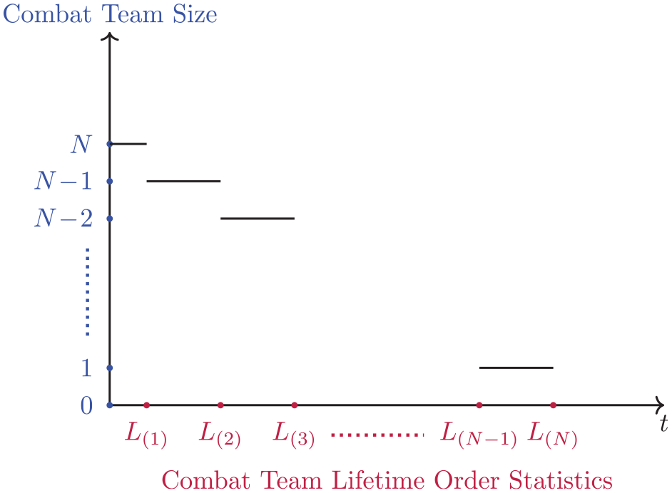
Combat team size variation with order statistics. The team initially has N members, and then after the first lifetime has expired, and the number of team members decreases by unity. This continues until the final lifetime expires and the number of team members reaches zero.

Note that more generally, the event that at least k team members are still alive at time t is equivalent to L ( N − k + 1 ) > t , for 1 ≤ k ≤ N , which provides a way in which partial combat team survivability may be quantified. For the case of identically distributed lifetimes, there is a closed form expression for the distribution of a general order statistic. ²⁷ If X 1 , X 2 , … , X N are independent and identically distributed statistics with common distribution function F X , then the i ^th-order statistic for 1 ≤ i ≤ N has distribution function

In some of the examples to follow, it will be shown how Equation (8) may be used to model the case where a combat team consists of collections of individuals grouped into sets which have identically distributed lifetimes.

The modeling methodology proposed in this study is illustrated schematically in Figure 2. It shows the mapping between combat team members (denoted S j for 1 ≤ j ≤ N ), their lifetimes ( L j ) , and an appropriate order statistic (in this case, L ( N − k + 1 ) for some 1 ≤ k ≤ N ). If this order statistic exceeds t , then there are at least k members of the combat team still alive at time t ; in the figure, N ( t ) is the number of team members still alive at time t .

OPEN IN VIEWER

Figure 2.

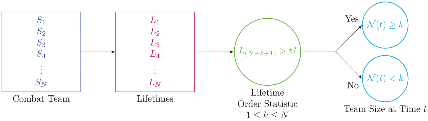
An illustration of the modeling process. The N combat team members are mapped to their lifetimes, and then, the ( N − k + 1 ) ^th-order statistic of their lifetimes is determined. If this is greater than time t , then the number of team members still alive at time t (denoted N ( t ) ) is at least k . Otherwise, there is less than k team members still alive at time t . If it is an operational requirement that at least k team members remain alive, then the model may be used to assess the likelihood of this occurring under various scenarios.

3. Series of examples

The following examples have been selected to provide an illustration of how the model developed in the previous section can be used to analyze BLUFOR team survivability. First, it will be shown how bounds on the Poisson arrival rate may be specified to ensure that BLUFOR survives intact with a pre-determined probability. Then, the analysis of the previous section will be applied in the case of attrition analysis of a large-sized BLUFOR where lifetime rates are based upon those in the work by O’Donnell and Blood ²³ and Zouris et al. ²⁴ Then, several cases will be considered to show how variations in BLUFOR member’s lifetimes may be introduced into the analysis. The rates provided by O’Donnell and Blood ²³ and Zouris et al. ²⁴ are for attrition per 1000 combatants per day. Hence, to express this for individuals in the models developed in this paper, units for α will be scaled by 1000.

3.1. Bounds on arrivals

Suppose that for BLUFOR to remain operational we required a survival probability of at least ϕ for the entire combat team. Hence, we require P ( L ( 1 ) > t ) ≥ ϕ . Then by applying this bound to Equation (6), one can show that the Poisson process arrival rate must satisfy the bound

λ ( t ) ≤ − log ( ϕ ) N − ∑ j = 1 N e − α j t .

(9)

This provides an upper bound on the Poisson process arrival rate to ensure that BLUFOR remains fully operational at time t . As a particular example, consider the case where N = 10 and each α j = 0 . 001 (so that rate of attrition is one combatant per 1000) with a constant Poisson mean of λ = 1 . Then with the requirement that ϕ = 0 . 9 , Figure 3 plots this constant rate and the bound to Equation (9). From the figure, it is clear that the critical point occurs at approximately time t = 10 , so that after this time the likelihood that BLUFOR survives entirely begins to drop below 0.9. The exact critical point can be shown to be given by

t critical = − 1 α log [ 1 + log ( ϕ ) λ N ] ≈ 10 . 59 ,

(10)

where this has been obtained by solving Equation (9) for t under the assumed conditions. This approach enables one to predict the time point where BLUFOR will begin to drop below its operational capacity. The methodology may be adopted to the case where BLUFOR is still functional even if it has lost some members. Specifically, note that the event { L ( k ) > t } is equivalent to the event that at least k team members are still alive at time t . Hence, if the team is still operational with a minimum number of members, this can be related to the corresponding lifetime order statistic and one may apply a similar analysis as in Equations (6) and (9) to determine bounds on the Poisson process mean arrival function.

OPEN IN VIEWER

Figure 3.

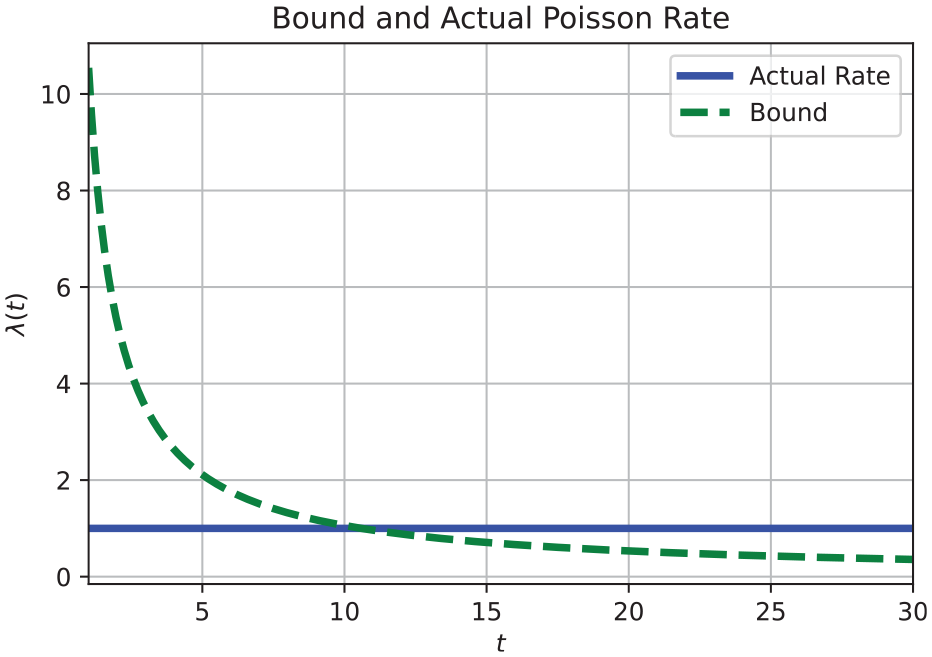
An example of the bound on the Poisson arrival process rate and the actual Poisson rate used in the corresponding example.

The next series of examples will assume a constant Poisson arrival rate λ ( t ) = λ . It is worth observing that if the Poisson arrival rate increases with time then BLUFOR survivability will drop rapidly, which is to be expected given the assumed lifetime model.

3.2. Examples with common lifetime rates

Consider the case where a common lifetime rate is assumed for a large fighting force of size N = 200 . KIA rates are provided by O’Donnell and Blood ²³ as mentioned previously. For combat troops deployed in Korea, the data set returned a mean attrition rate of 0.209 per 1000 troops, while for the Okinawa data, it is 1.42 per 1000 troops. Combat support troops attrition rates are also available but are not included in this analysis. These rates are then expressed as rates for individuals, so that α Korea = 0 . 209 × 10 − 3 and α Okinawa = 1 . 42 × 10 − 3 , and Figure 4 plots the probability that the entire BLUFOR is still functional at time t . This is under the assumption of a constant REDFOR arrival rate of 20 combatants per unit time. The figure shows that survivability in Korea has a higher probability than that in Okinawa and that BLUFOR is more likely to survive intact in the Korean example. When the REDFOR arrival rate is reduced, the model reflects the expected behavior that survivability is increased for both cases. Likewise, when the arrival rate is increased the time window where BLUFOR remains intact reduces rapidly.

OPEN IN VIEWER

Figure 4.

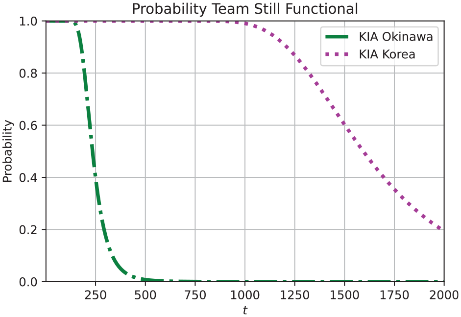
BLUFOR survival when REDFOR has an arrival rate of 20 combatants per unit time, based upon the two KIA data sets.

WIA rates are provided in both the work by O’Donnell and Blood ²³ and Zouris et al. ²⁴ For the Korean data, the individual rate is α Korea = 2 . 853 × 10 − 3 , while for Okinawa, it is α Okinawa = 6 . 86 × 10 − 3 . In the work by Zouris et al., ²⁴ a number of WIA rates are provided for different battles. Here, only two have been utilized. In the first case, the second battle of Fallujah has a rate of α OIF = 1 . 04 × 10 − 3 , while for OEP, the peak casualty rate is α OEP = 1 . 02 × 10 − 3 . Figure 5 plots the probability that the entire BLUFOR combat team survives over time, based upon the four WIA rates. The figure shows that for the OIF and OEP campaigns it was more likely that BLUFOR survives entirely than in the Korean and Okinawa battles. This may be explained by the fact that there have been significant technological innovations between the two groups of wars, resulting in increased likelihood of individual combatant survivability.

OPEN IN VIEWER

Figure 5.

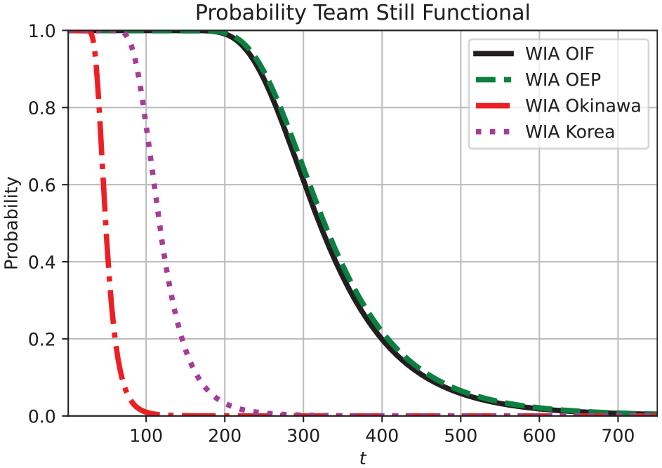
BLUFOR survival when REDFOR has an arrival rate of 20 combatants per unit time, based upon four WIA data sets.

3.3. Examples with common lifetime rates

To illustrate Equation (6) under different conditions suppose that N = 8 with α j = j × 10 − 3 for each j ∈ { 1 , 2 … , 8 } . N has been chosen to reflect a smaller fighting force and to facilitate the numerical analysis, while the selections for the α j have been motivated by the choices discussed previously. Figure 6 plots Equation (6) for the cases where λ = 0 . 1 , 1 , and 2. The figure shows that despite the fact that the BLUFOR parameters α j are small (implying larger mean lifetimes initially), as the rate of REDFOR arrivals increases the probability of complete BLUFOR team survivability decreases. Since N has been selected to be small, if the rate of arrivals of REDFOR exceeds the size of BLUFOR initially then the latter’s survivability will be reduced significantly, in view of the lifetime model (Equation (2)).

OPEN IN VIEWER

Figure 6.

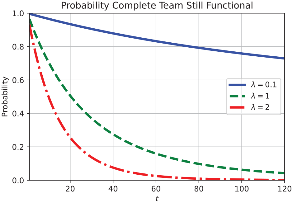
An example where N = 8 , BLUFOR has different lifetime parameters and for three REDFOR arrival rates.

3.4. Different subgroups illustration

So far the analysis has focused on BLUFOR consisting of a group of homogeneous individuals with potentially different inherent lifetime parameters. One can instead suppose that the combat team consists of a series of subgroups with common lifetime parameters but such that a given minimum number from each subgroup is required for the team to remain functional. To clarify this, the team may consist of a subgroup of specialized medical, logistic, and communications personnel, in addition to regular combat troops. Out of each subgroup, the team may remain operational only if at least 70% of each subgroup remains, for example. Hence, it is useful to extend the previous analysis to such a situation.

Suppose that the BLUFOR combat team consists of M subgroups, each containing M i members for i ∈ { 1 , 2 , … , M } . Assume that within each subgroup the individuals are homogeneous with lifetime parameter α j and that the underlying lifetime models are independent. For each subgroup, it is supposed that the team remains functional provided at least k j members are still alive at time t . Then, subteam j is still operational at time t if the ( N − k j + 1 ) ^th-order statistic exceeds t . Denote by X ( k j , M j ) this order statistic of the lifetimes. Then, the probability that subgroup j is still functional at time t is P [ X ( k j , M j ) > t ] , and under the assumption of independence of subgroups, it follows that

P ( BLUFOR functional at time t ] = Π j = 1 M P [ X ( k j , M j ) > t ] .

(11)

One may apply Equation (5) for each subgroup and then utilize Equation (8) to provide inputs into Equation (11).

To illustrate this, consider the following example. Suppose that BLUFOR consists of M = 4 subgroups with M 1 = 6 , M 2 = 8 , M 3 = 5 , and M 4 = 7 . Assume that k 1 = 4 , k 2 = 5 , k 3 = 4 , and k 4 = 3 , and α 1 = 0 . 001 , α 2 = 0 . 002 , α 3 = 0 . 01 , and α 4 = 0 . 02 . Then, Figure 7 plots the probability that the combat team remains functional over time t for three different constant Poisson arrival rates, namely λ = 0 . 1 , 1 and 2. As can be observed as the Poisson rate increases the likelihood of the team remaining functional decreases rapidly. The larger lifetime rates (for subteams 3 and 4) contribute to this rapid decline. To demonstrate this, Figure 8 repeats the same experiment except α 3 = 0 . 001 and α 4 = 0 . 002 and shows a significant improvement in the likelihood of team survivability over longer time frames.

OPEN IN VIEWER

Figure 7.

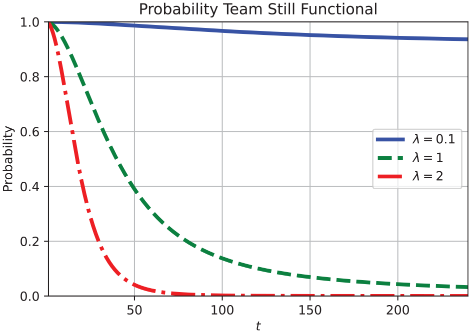
Analysis when BLUFOR consists of four different subgroups with different lifetime parameters.

OPEN IN VIEWER

Figure 8.

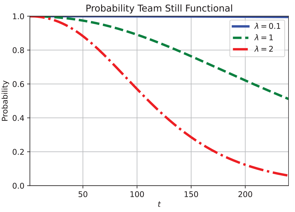
Similar analysis as in Figure 7 except initial mean lifetimes is all large.

3.5. Lifetime correlations

Throughout the analysis, all individual lifetimes have been assumed to be independent. One can also consider the case where lifetimes are in some way correlated. Instead of just assuming that there is an underlying common correlation among the entire team, one may instead consider groups that contain statistically related members. To do so, it will be supposed that BLUFOR contains a series of independent subgroups of two individuals, and impose a correlation structure within these subgroups. This requires the specification of an appropriate bivariate distribution for pairs of lifetimes, whose marginal distributions match that specified by Equation (5).

To facilitate this, we suppose that the Poisson rate is constant, so that λ ( t ) = λ . Then, it is possible to invert the distribution function (Equation (5)) so that it may be simulated through a uniform random variable and through the inverse transform algorithm. ²⁸ This can then be related to an exponential distribution with appropriate parameter through the same transformation method. Consequently, one can demonstrate that lifetime L j is equivalent to

L j = − 1 α j log [ 1 − α j λ Y j ] ,

(12)

where Y j has an exponential distribution with parameter α j . This expression indicates that one may generate correlated lifetimes through a functional transformation of correlated exponential random variables. To illustrate in the bivariate case, it can be shown that the bivariate survivor function of lifetimes L i and L j is

P [ L i ≥ x , L j ≥ y ] = P [ Y i ≥ λ α i [ 1 − e − α i x ] , Y j ≥ λ α j [ 1 − e − α j y ] ] ,

(13)

where the right-hand side of Equation (13) is the survivor function of the bivariate exponential distribution ( Y i , Y j ) .

There are many bivariate exponential distributions from which to choose, such as Gumbel’s ²⁹ and Hougaard’s, ³⁰ and others documented by Nadarajah and Kotz. ³¹ Although it is relatively straightforward to postulate parameters for univariate statistical models of lifetimes, the selection of an appropriate correlation structure is much more complex. This is because there can be significant variation in the structure of a combat team which can determine local dependencies between lifetimes.

Hougaard’s bivariate exponential distribution is adopted in the examples to follow. This model has joint survivor function

P ( Y 1 > t 1 , Y 2 > t 2 ) = e − { ( α 1 t 1 ) r + ( α 2 t 2 ) r } 1 r ,

(14)

For a constant r > 0 , with a correlation coefficient given by

ρ = Γ 2 ( 1 / r ) r Γ ( 2 / r ) − 1 ,

(15)

where Γ ( · ) is the gamma function. It can be shown that the marginal distributions of Y 1 and Y 2 are exponential with parameters α 1 and α 2 , respectively. By an application of Equations (14) to (13), one arrives at

P [ L i ≥ x , L j ≥ y ] = e − λ { ( 1 − e − α 1 x ) r + ( 1 − e − α 2 y ) r } 1 r ,

(16)

producing the survivor function for the joint lifetime distribution, which by construction will possess marginal distributions of the form (Equation (5)). Determining this transformed distribution’s correlation is somewhat difficult analytically, but under parameterizations of interest an approximate rule of thumb may be established. Observe that in view of Equation (12), under the assumption that λ > > α j , one may apply a linear approximation to show that the lifetime is a constant times the exponential distribution. This means that the correlation associated with the marginal distributions in Equation (16) will be preserved from Equation (14). Consequently one may use Equation (15) as an approximation to the true bivariate distribution’s correlation. The assumption upon which this analysis is based is plausible since λ is the Poisson mean arrival rate and the reciprocal of α j is the mean lifetime parameter, so cases of interest will occur under the aforementioned condition.

In the analysis to follow, team survivability will be examined only through the condition that all members of the team survive to time t . This means that the first-order statistic of lifetimes may be employed as previously. In terms of pairs of correlated lifetimes, the probability that the minimum exceeds t can be derived by evaluating the survivor function (Equation (16)) at x = y = t .

To provide an example suppose that BLUFOR consists of eight members, grouped into subgroups of two, such that lifetimes are independent between subgroups but within each subgroup the lifetimes are governed by the bivariate distribution (Equation (16)). For simplicity suppose that the lifetime parameters within each subgroup are identical. In particular, group A has α A = 0 . 0001 , group B has α B = 0 . 0002 , group C has α C = 0 . 0003 , and group D has α D = 0 . 0004 . Three cases of Poisson mean arrival rate will be considered, namely λ ∈ { 0 . 01 , 0 . 1 , 1 } which will imply the correlation approximation should be valid. The probability of team survivability at time t will be the product of survivor functions (Equation (16)), evaluated at x = y = t , over each respective team. As a benchmark, Figure 9 plots the probability of team survivability for the case where r = 1 , which corresponds to the uncorrelated case (and independence in this situation). For a comparison, consider Figure 10 where r = 4 with a correlation of ρ = 0 . 8541 . Comparing these two figures, it is clear that as the REDFOR arrival rate increases the effects of correlation result in a decline in the number of BLUFOR members over time.

OPEN IN VIEWER

Figure 9.

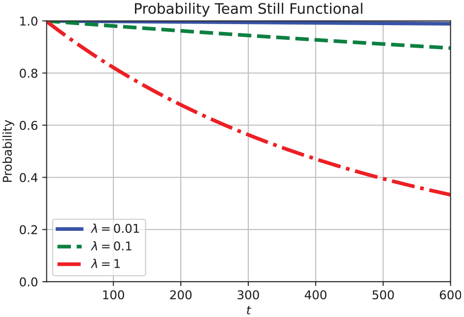
BLUFOR survivability when it is composed of subgroups of two individuals, in this case with uncorrelated lifetimes.

OPEN IN VIEWER

Figure 10.

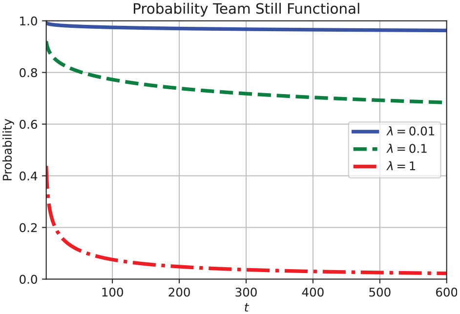
A repeat of the scenario in Figure 9 except that each subgroup of two has a significantly large correlated lifetime through the bivariate lifetime distribution.

4. Conclusion

The objective of this paper was to introduce a stochastically driven approach to model combat attrition between comparable fighting forces, motivated by underlying assumptions in the formulation of the well-known Lanchester’s equations. An exponential distribution was specified to model individual lifetimes, whose conditional mean varied inversely with the size of the opposite fighting force. Based upon the assumption that REDFOR arrivals are Poisson distributed, the corresponding lifetime model was produced for BLUFOR members. These modeling assumptions were justified by reference to data analysis studies. An order-statistic approach was utilized to show how full BLUFOR survivability could be related to specific order statistics. Examples were used to show how analysis could be undertaken, including the case where pairs of BLUFOR members shared correlated lifetimes. This new approach to modeling combat attrition allows more flexibility than is possible through Lanchester’s equations.

It would be of interest to validate this approach with further analysis of combat attrition data, as well as the application of the approach to analyses such as those examined by Kress ⁸ and Adams and Mesterton-Gibbons ¹⁴ The methodology could also be applied to study attrition in swarms of drones. Further to this, development of a more refined model for correlated lifetimes would enhance these studies.