
Abstract
Since the 1970s advances in science and technology during each succeeding decade have renewed the expectation of efficient, reliable automatic epileptiform spike detection (AESD). But even when reinforced with better, faster tools, clinically reliable unsupervised spike detection remains beyond our reach.
Expert-selected spike parameters were the first and still most widely used for AESD. Thresholds for amplitude, duration, sharpness, rise-time, fall-time, after-coming slow waves, background frequency, and more have been used. It is still unclear which of these wave parameters are essential, beyond peak-peak amplitude and duration. Wavelet parameters are very appropriate to AESD but need to be combined with other parameters to achieve desired levels of spike detection efficiency.
Artificial Neural Network (ANN) and expert-system methods may have reached peak efficiency. Support Vector Machine (SVM) technology focuses on outliers rather than centroids of spike and nonspike data clusters and should improve AESD efficiency. An exemplary spike/non-spike database is suggested as a tool for assessing parameters and methods for AESD and is available in CSV or Matlab formats from the author at
INTRODUCTION
Seven years following the publication of Hans Berger's first paper describing the human EEG in 1929, the association of EEG spikes with epilepsy was published by Fred Gibbs, William Lennox and Erna Gibbs. In the decade to follow the visual characteristics and clinical correlations of spike activity were described and exist today, seven decades later, essentially unchanged.
I saw my first human EEG spike in 1953 in a hospital setting and began studying epileptiform activity in animals with analog frequency analysis in 1955 1,2 . It was nearly 20 year later when the acquisition of a small digital computer (8k of memory!) allowed our laboratory and others to detect and display paroxysmal (spikes) and non-paroxysmal waves in real time. Since then, clinicians and engineers have applied increasingly sophisticated computer algorithms to the problem of Automatic EEG Spike Detection (AESD, or just “spike detection”), by which we mean the use of digital computer algorithms to detect epileptiform spikes, i.e., spikes having a waveform usually associated with underlying epileptogenic activity in the brain.
The “old ones” of North American clinical EEG (e.g., H. Jasper, F. Gibbs, W. Lennox, R. Schwab, C. Henry, J. Knott) sometimes would define a spike as “something that would hurt if you sat on it.” This statement has three implications: First it emphasized the relative isolation of spikes in time, the steep rising and falling slopes of a spike and the most common spike appearance as an upright, predominantly negative EEG feature. Second, it underlined our lack of understanding of the human visual pattern recognition process since we could not do any better than use an analogy to describe what we were seeing. Third it suggested that spike detection might be simple, that anyone could do it once they “got the hang of it.” Indeed, generations of EEGers learned to recognize spikes, some better than others, but all better than any of the computer-based detection systems devised since then.
Two decades later Celesia and Chen 3 studied 600 spikes in 100 patients. Four parameters were analyzed visually (polarity, amplitude, duration and sequence), and the main characteristics of epileptiform spikes were summarized: “88% of spikes were negative. 98% of spikes raised 30% above the background activity. Spike duration varied, the shortest spike had a 9 msec duration. The range of duration varied from 9 to 200 msec with a mean of 45.06. 75% of spikes were followed by a deflection lasting from 130 to 200 msec.”
Four years later Gotman provided quantitative measurement of Spike morphology. 4
The advent of each new technical advance, each new method of analysis, each new opportunity for EEG data collection, has led to a flurry of applications for AESD. There are a few groups that have maintained a persistent interest in AESD. Many researchers in this field are budding engineers or clinicians with computer credentials who recognize the importance and relevance of AESD for clinical application and seem to think, individually and collectively, that “spike detection can't be that difficult.” But it is difficult, as evidenced by the fact that no completely satisfactory program for AESD is presently available. This body of work has been well reviewed by Frost, 5 Ktonas, 6,7 Lopes da Silva, 8 Gotman 9 and Wilson and Emerson. 10 The reader is referred to these excellent sources for additional references and detail of work done in the 20th century.
The following discussion will describe the spike detection problem and the different approaches to AESD with a view toward learning from the successes and failures of each and developing a point of view that may enhance the likelihood of further progress in AESD. Then we will apply what we have learned to a problem set in spike detection and begin to see for ourselves what works, what does not and why.
THE PROBLEM
Spikes are truly needles in the proverbial haystack of nonspike activity. A 20-minute 19-channel clinical EEG with a clear left temporal spike focus might have 100 spikes distributed across several channels that must be distinguished from 228,000 nonspike events (estimating 10 such event/sec), a probability of p=0.00044. This means that low probability spike-like features that occur as outliers (for example high amplitude bursts of alpha activity) in ongoing EEG activity will often be more frequent than the sought-after spikes. We can be clear that we do not have to detect all spikes for a clinically effective detection system since clinical EEGers have difficulty reaching agreement on any but the biggest spikes (Wilson, et al. 11 ). But we would like to detect nearly 100% of big, obvious consensus spikes.
The false detection problem is even worse. A false detection rate of 1:1000 in the above example would generate 228 false detections, more than twice the number of spikes. Some studies report only sensitivity and false positives per minute because they lack data on the actual number of events analyzed.
Table 1 shows a hypothetical two-by-two table of spikes vs. detections from a total of 1000 events. The spike prevalence is 10/1000, 1 %. High values for sensitivity and specificity suggest high efficiency in detecting spikes. However, because of low spike prevalence these statistics are very misleading.
Statistical measures of spike detection when nonspikes are much more frequent than spikes
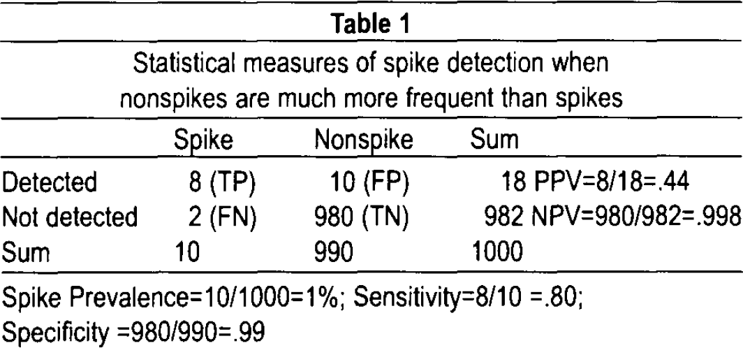
Spike Prevalence=10/1000=1%; Sensitivity=8/10 =.80; Specificity =980/990=.99
When evaluating spike detection efficiency in the face of low spike prevalence, most often the case in the clinical EEG setting, the positive predictive value(PPV=TP/(TP+FP, sometimes called selectivity) is a better reflection of detection efficiency. In this example, if a sensitivity of 80% and a specificity of 99% are associated with a spike prevalence of 1%, the PPV is reduced to 44%. This means that any detected event is more likely to be a nonspike than a spike! From the practical standpoint when spikes are common (prevalence >1%) we need a high PPV, say 90% or more, to avoid being overwhelmed with a large number of nonspike detections. On the other hand when spikes are rare (prevalence < 0.1%) a PPV of less than 50% might be tolerable since the actual number of false detections to deal with might be acceptably low. Two points are to be made: (1) spike prevalence and PPV should be reported and evaluated along with sensitivity and specificity in order to allow comparison of different methods of spike detection, and (2) clinical judgment is required to decide whether or not a particular PPV is acceptable for a particular application.
We will see that these basic statistical issues continue to be central to the development of methods, evaluation of performance, and the clinical application of AESD, from the earliest studies up until the present time. 12 Most published work does not address these issues, and is therefore difficult to evaluate (see Wilson's papers 10,11 and Argoud et al. 13 ).
DEVELOPMENT
The history of AESD can be grouped into three periods: (1) beginnings, 1972–1985, the widening availability of small special-purpose laboratory computers and the publication of initial papers on AESD; (2) new technologies, 1985–2002, the application of neural networks and wavelet transforms to spike detection, and (3) the present, 2002–2009, the sobering recognition that fast computers and new classification algorithms are not resolving the problem of spike detection.
Beginnings 1972–1992
In the early 1970s Carrie, 14 –16 Gotman, 14 –16,17 –24 Harner, 19 –22,25,26 Ktonas, 27,28 Samson-Dollfus, 29 Zetterberg 30 and their colleagues began developing spike detection applications using interval-amplitude analysis. Wave extrema (peaks and troughs) and/or zero crossings were used to define half waves and whole waves for each EEG channel. Plots of amplitude vs. duration for all waves showed a few spikes well outside the more compact clusters of background activity in selected samples (Figure 1, left) and suggested good potential for separating/detecting spikes. 25 Maps at right show location of spikes and associated reduction of alpha activity over the right hemisphere.
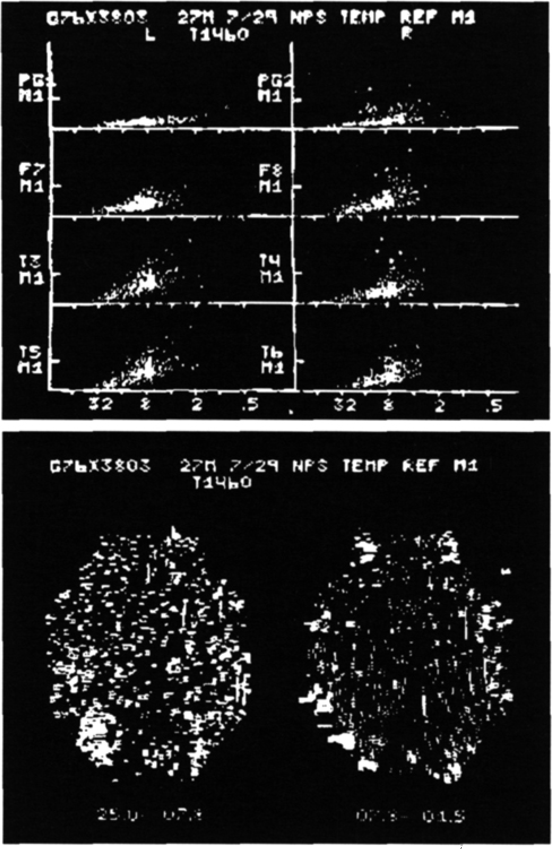
Real-time 8-channel automatic spike detection (PDP8 minicomputer) and topography (oscilloscopic display, Polaroid®), 1976. At top, half waves are plotted in 8 topographically-arranged amplitude-duration graphs. Y-axis is marked at 50 μV. X-axis labeled with frequency equivalents of log2 duration. Large dots (mainly at F8 and T4) represent detected spikes much larger than background (small dots). At bottom, same data displayed in alpha/ beta and theta/ delta maps (background=horizontal lines proportional to duration, spikes=vertical lines proportional to amplitude).
Based on amplitude, duration, sharpness and other parameters Gotman and Gloor 17,18 developed a threshold-based expert system algorithm that was subsequently ported to commercial systems and became the de facto standard against which all subsequent detection algorithms would be judged. While spikes could be detected, false positives were numerous and prevented widespread acceptance and application. Performance of this standard method left enough room for improvement to encourage others to try their hand. In Gainesville (Florida) Smith and Ktonas 28 developed a very detailed set of spike waveform parameters in hope of improving the detection process. Autoregressive parameters were also tested by Lopes da Silva in Amsterdam. 31 Neither group's result surpassed the Gotman algorithm performance. Carrie and Harner did not extend their projects.
Harner 21 and Celesia 3 had suggested the sequence of wave segments EEG waveforms might provide useful information in the context of spike detection. In two papers Faure 32,33 and Samson-Dollfus in the Rouen (France) group reported the application of syntactical analysis of wave sequences for spike detection. There has been surprisingly little follow-up of this line of research, an intriguing subject that deserves further attention in AESD.
Frost and Ktonas 34,35 ended up working together on the context in which spikes occur. Gotman extended his work to spike-wave and seizure detection and formed his own company to further his work in EEG analysis. In 1991 he added patient state as a context parameter to reduce false positive spike detections. 36,37
A number of other papers addressed a wide range of subjects including spike-wave detection, mapping of detected spikes, elimination of false positives, clinical correlation of spikes, long-term monitoring and computational methods. 8,18,26 –38 –53
Every interested party thought that the problem of further improving AESD would be resolved by faster computers and better algorithms. An early single paper applied discriminant analysis to spike detection. 54 There were few responses or follow-up papers. In the 1980s, fueled by increasingly available computer power, wavelet transforms and self-learning computer-based artificial neural networks were developing. And that is where the matter rested until 1992.
New technologies 1992–2002
Artificial Neural Networks (ANN)
During training on known events (spikes) ANN algorithms compute relative weights for input parameters in order to compute linear weights for one or more outputs that then are used to separate events of interest from other events. Training may be quite slow depending on the number of parameters and the number of events to be analyzed. However, once output weights are obtained from training, analysis of new data is extremely fast, easily allowing real time application.
When too many input parameters are used, ANN may correctly classify all events during training but the resulting output parameters will not work for new data (overfitting and poor generalization). A second issue with ANN derives from the fact that information about the weight given to individual input parameters is usually buried in one or more layers of the algorithm and not retained by ANN. This makes it hard to select the best parameters to improve classification and prevent overfitting. The best parameters will be those which apply to most, if not all spikes. Large numbers of parameters that relate to only a few spikes are likely to result in overfitting and poor generalization. Recently, there have been attempts to extract the input weight information by monitoring the very large numbers of interconnections within the ANN algorithm. So far the proposed extraction methods are simplistic, computationally demanding or lacking in rigor, leaving us without the information needed to optimize input parameters for AESD.
In 1992 Gabor and Seyal 55 applied a state-of-the-art linear ANN algorithm to spike detection and achieved a sensitivity of 94 ± 7% and selectivity (PPV) of 71 ± 23%. The idea was, and is, that a self-learning algorithm should be able to weigh multiple parameters for spike classification better than any expert trying to set the parameter weights and thresholds based on instinct or experience. Others were encouraged to try ANN for EEG spike detection and a number of additional papers resulted with similar results. 56 –63
Wavelets
In 1992, Senhadji, 64 a young engineer in Renne 65 first applied time-frequency analysis to AESD, using wavelet methods that had been developed in France during the preceding decade by Grossman and Morlet, 66 Daubechies 67 and Mallat. 68
Wavelets and time-frequency analysis are methods that convert an EEG signal into a 2-dimensional map of time vs. wavelets or frequencies. For frequency analysis sine waves representing a range of frequencies are fitted to the signal. With the wavelet transform a chosen set of single waveforms, the wavelets, are fitted to the signal. The choice of waveform for the wavelet is not trivial. Often an oddly-shaped wavelet is chosen so that each of wavelets in a set will be statistically independent of the others (orthogonal), valuable for subsequent analysis (and very different from classical frequency analysis by the Fourier Transform). There is no reason not to choose a set of wavelets for spike detection that look as much as possible like spikes (see Argoud, below).
These wavelet maps have much more temporal resolution than frequency power spectra but still much less than the original spike signal. Since wavelet transforms were found to be of great value for data compression in image processing, it was hoped that the wavelet parameters of scale and detail (amplitude and time distribution) would have similar value in spike description and detection. However interesting and intriguing this hope, this and subsequent papers showed little additional benefit over the methods based on the original parameters selected by Gotman and colleagues.
Wilson and Emerson 10 weighed in heavily in their review of 25 previous papers. They concluded that (1) even the EEG experts are not all that expert in spike detection (Wilson et al. 11 ); (2) few studies provide sufficient data to allow comparison with other studies (see above); (3) clustering of detected “candidate” spikes so that they can be evaluated by an expert may have some time-sparing benefit.
Even with the addition of wavelets, ANN, and clustering to the computational armamentarium, AESD had not improved enough to come into general use.
The present, 2002–2009
Since the 2002 review there have been a number of papers on AESD. The majority presented new computational approaches. 69,82 Others extended old approaches. 74,83 –88 A few addressed the comparison of different AESD algorithms. 12,89 –92 One paper compared the performance of ANN on spike detection using three sets of selected input parameters or raw data for input and found no significant difference among the four groups. The unavoidable conclusion is that none of the proposed methods for AESD has been shown to be “ready for prime time.”
Perhaps most encouraging is a paper from Brazil 13 that used 1) wavelets chosen to resemble spikes, and 2) ANN classification to analyze (3) 4765 spike-seconds from (4) 9000 minutes of recording. They achieved 71 % sensitivity, 99% specificity, a PPV of 80% and a false positive rate of 0.13/m. From these data it is possible to approximately construct a spike detection table that we can use as a model for evaluating the efficiency of this and other AESD methods (Table 2). The spike prevalence is high (5.3%), which partly accounts for the relatively high PPV.
Spike detection statistics reconstructed from Argoud et al. 13
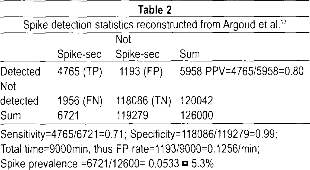
Sensitivity=4765/6721 =0.71; Specificity=118086/119279=0.99; Total time=9000min, thus FP rate=1193/9000=0.1256/min; Spike prevalence =6721/12600= 0.0533 = 5.3%
Even these good results would probably disappoint a clinical electroencephalographer because the method missed nearly a third of the expert-verified spikes and still misidentified 20% of the detections as spikes. This is probably about as good as one can do using wavelets and ANN, the most popular of new parameters and new methods. Since wavelet parameters are not known to be optimal, further improvement without overfitting might be possible by replacing inefficient wavelet parameters with efficient ones of another type. And perhaps other self-learning algorithms can be found that will prove to be better adapted to the special problems of AESD than is ANN.
Parameter improvement
Faced with insufficient information to cull optimum input parameters for AESD from those suggested by experts from different fields, EEG informaticians have tended to stick with parameters that seem promising, such as wavelets. Another approach involves separating the EEG into components or features, typically using singular value decomposition (SVD). ICA (Independent Component Analysis) is a newer method of finding components of interest. ICA is of particular interest for spike detection since its classification algorithm is based on minimizing kurtosis. Kurtosis is a function of the 4th power of the signal and is therefore a measure of “sharpness” that should be particularly apt for spike detection. Both SVD and ICA can reduce the number of inputs to a neural network and reduce overfitting. ICA may do a better job of emphasizing spike activity.
Along the same line the Nonlinear Energy Operator (
Finally, it is now computationally feasible to use all parameters that might conceivably be useful as input to a neural network. Redundancy is an issue but can be reduced by some type of factor analysis (e.g., Principle Component Analysis, PCA) that eliminates components which contribute little or nothing to the overall variance or information content. We can make the case that a search for better AESD parameters is more likely to be rewarding than searching for a better AESD algorithm. For example, we recently compared an ANN method to a version of the Gotman algorithm (a threshold-based expert system, somewhat enhanced by using a Bayesian summation of probabilities), using the same parameters. While sensitivities for both were improved compared to the available commercial methods, false positive detections were numerous. The new ANN method was no more efficient than the enhanced heuristic method (Minasyan G. and Harner R., 2005, unpublished).
Algorithm improvement
In the latter regard it is useful to address two characteristics of most data clustering algorithms (cluster analysis, Bayesian analysis, PCA, ANN, etc): (1) clusters of events are characterized by their centers (centroids) and (2) the distances between centroids is determined by linear weights (simple multiplication) of output parameters. One may begin to think of the detection process as one of drawing a line between a cluster of spikes and a cluster of nonspikes on a graph of amplitude vs. duration. (A plane is needed to separate spike clusters from nonspikes characterized in three dimensions by amplitude, duration and sharpness. And an unvisualizable hyperplane is the required separator for 4 or more parameters). When the clusters are close together outliers from each group may be misclassified by falling on the “wrong” side of the separator. The separation process is greatly improved by choosing parameters that increase separation between centroids and/or reduce variability (fewer outliers) within spike and nonspike clusters. Nonlinear ANNs are mostly theoretical but the use of nonlinear input parameters (squares, NLEO, reciprocal, first derivatives) is a substitute that so far does not seem to improve matters. This leaves us with finding a replacement of cluster centroids as a means of separating clusters. Centroids define exemplary spike and exemplary nonspikes and are not focused on the outlying borderline cases of spike and nonspike events of interest to clinical EEGers. Support Vector Machine (SVM) 72,93 technology addresses this issue and has recently been applied to spike detection. The basic idea is to adjust the position of the separator (line, plane, hyperplane) between spike and nonspike clusters based on the distance from misclassified outliers, exactly what we would want for spike detection. We should expect some improvements in spike detection statistics as SVM technology is increasingly applied to AESD.
FUTURE PROSPECTS
Goals
The first thing we might do is reevaluate our goals. If achieving the accuracy of expert spike detection with AESD turns out to be beyond our capacity, one approach would be to focus on the largest most easily detectable spikes for detection, mapping, dipole analysis and the like. Another would be to hybridize the process and expand practical methods for submitting spike candidate to expert review, as has been done in at least one commercial system.
If we retain the goal of achieving or exceeding expert levels of spike detection with AESD, then we need to find some new ways of looking at our data, our parameters, our analyses, and our results with a view toward optimization at each stage in the detection process. This means reevaluating our choices for data input, monitoring our analytic choices at each step of the way, and retaining complete statistics for comparing performance of competing AESD methods. Particularly the first two of these may be considered daunting but Exploratory Data Analysis (EDA) 94,95 is an approach to both developed by John Tukey (originator of the FFT) that may be helpful.
EDA and Spike Detection
The core principle of EDA is the use of data visualization, graphics, to enhance our understanding of patterns and distributions as a guide to further analysis. This would seem to be a particularly satisfying option for those of us who are very comfortable with visual pattern recognition as applied to EEG or for whom the above discussion of algorithms, clusters and hyperplanes is mind-numbing. As a demonstration of the potential for EDA in spike detection we will present a small data set of “consensus” spikes and nonspikes, show the effect of data scaling and transformation on waveforms and two dimensional clustering and then evaluate a few different types of parameter for spike detection.
Basic Spike/NonSpike data set
For this demonstration we limit the scope of the detection problem to finding “consensus spikes” that would be agreed upon by a great majority of experts, without regard to clinical correlation, location, number of channels involved, equivalent source localization, and the like. If a spike can be seen and distinguished by experts it should be possible to detect it automatically in a single second from a single channel. Once this limited, achievable goal is achieved, further detection and localization of spikes beyond the capability of experts can be attempted. Reliable consensus spike detection that emulates the best of experts on the best of days will have clinical utility, particularly when scanning numerous or long-term EEG recordings where mood, fatigue, boredom and distraction diminish expert performance.
We recognize the importance of context in the process of visual EEG interpretation. Same channel and adjacent channel features, along with clinical state features provide useful detection and confirmation filters for spike detection. Still, the first step is to detect the obvious visual pattern. Once spikes have been detected in short samples, context features may be applied to enhance the interpret-ability, localization and functional significance of spike data.
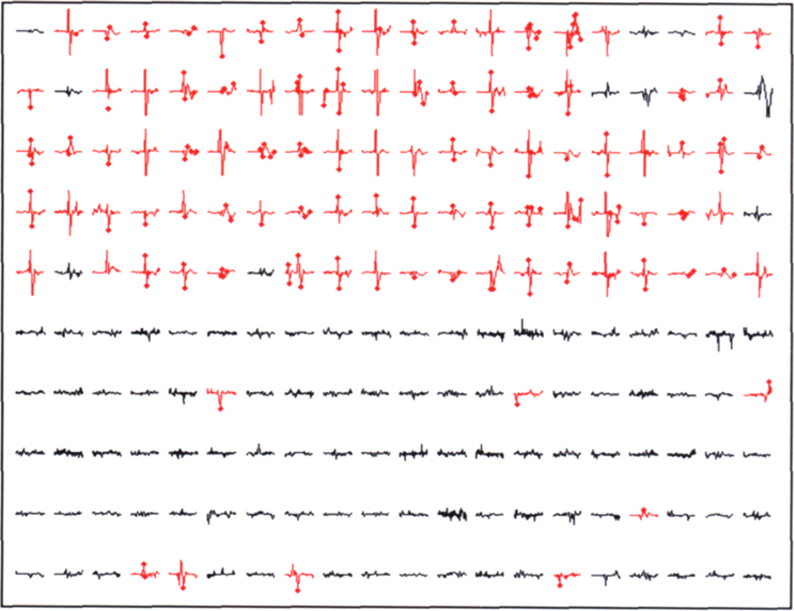
We begin by looking at 100 1-sec spike and 100 nonspike samples (Figure 2) and posing the following problem: how many of the spikes can be detected by an AESO program/method that produces few or no false detections in the nonspike EEG samples. The maxima and minima are indicated with a large dot. Note that most but not all of the spikes are detected as a maximum or minimum value.
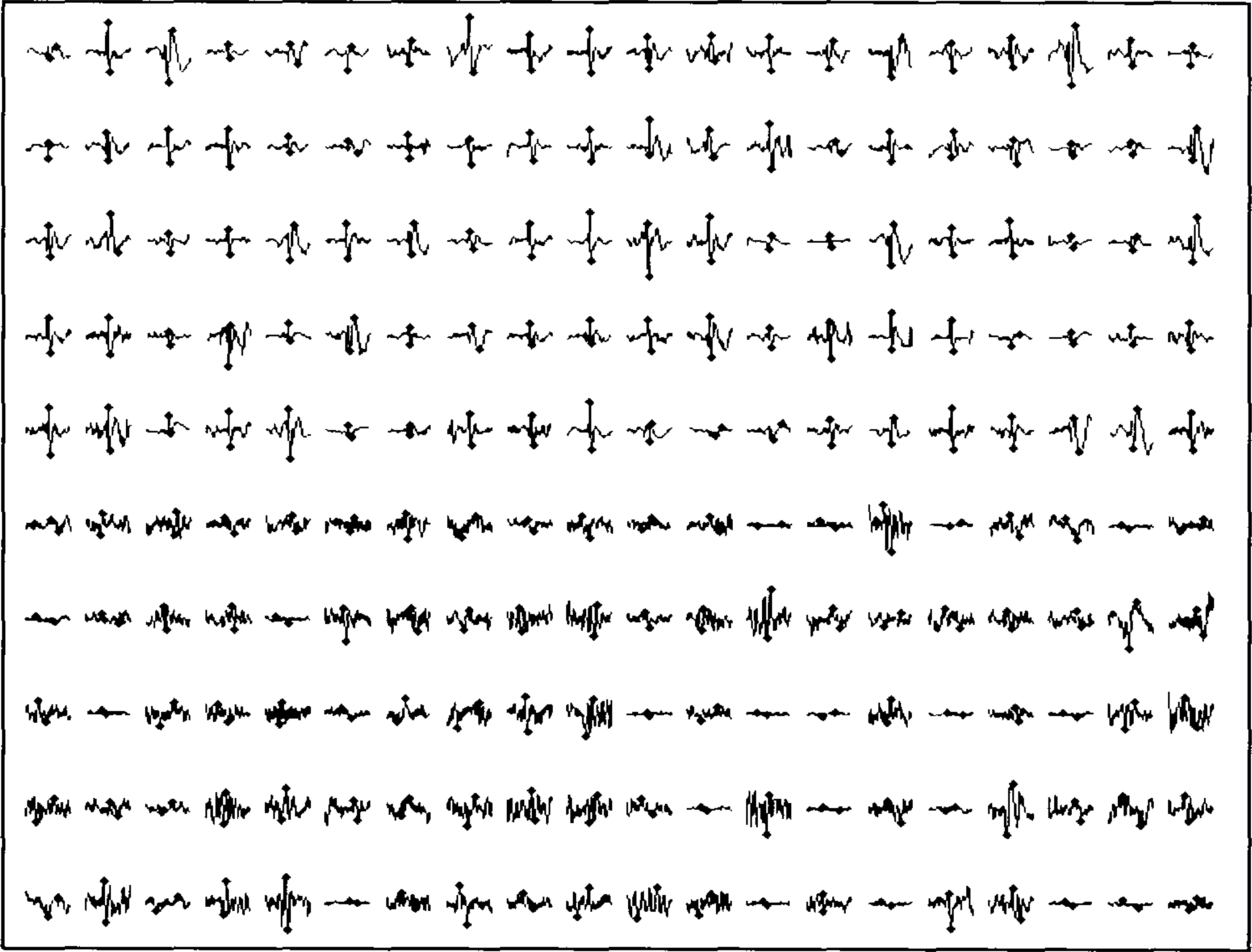
Thumbnail display of 100 Spikes (top 5 rows) and 100 NonSpikes (bottom 5 rows) in 1-sec epochs (200 samples/sec), no scaling. Maximum and minimum values for each epoch are indicated. Most, but not all, maxima/minima are associated with spike peaks, near the center of Spike epochs, and widely distributed in NonSpike epochs.
Review the samples in Figure 2 which are offered as consensus-building data. If you identify any Spike sample that you think is not a Spike or any NonSpike that you think is a Spike, then I will not have done a good job of consensus-building. As you evaluate the discussion to follow below, you may want to exclude the samples with which you disagree from the data.
We can anticipate problems with each of the current approaches to AESD described below. Heuristic (rule-based) methods often will be at a loss to find parameters that, singly or in combination, separate spikes from confounding nonspike features. Some methods may find the short sample duration of 1 sec to be limiting or insurmountable.
Data scaling
Iindiviual normalization of each epoch prior to analysis is desirable because EEG amplitudes in general and spike amplitudes in particular vary widely as a function of subject, clinical state, channel, and source localization. Therefore, programs for AESD must be designed to work with relative amplitude. Absolute amplitudes can be retained and used for specific purposes later in the process as desired.
Normalization involves division of all sample points by a central measure of amplitude, for example the mean, mode, median, or standard deviation (SD). The SD is often used for such purposes but in fact is quite inappropriate since large outliers like spikes skew the distribution of EEG amplitude and shift the SD away from the main body of background activity. The median is insensitive to infrequent outliers and may be chosen as a robust measure of background amplitude for each epoch. Note that the median is taken from the absolute (unsigned) EEG amplitudes, otherwise the result would be close to zero.
Figure 3 shows superimposed Spike and NonSpike epochs. This display was first used by George Dawson in 1947 as a photographic method of averaging evoked responses. The Dawson display has the advantage of displaying signal variability as well as the average values. We see that variability is reduced before spikes and increased afterward. Particularly when spikes are large the associated alteration in background activity can easily be seen, increased slowing and decreased fast activity.
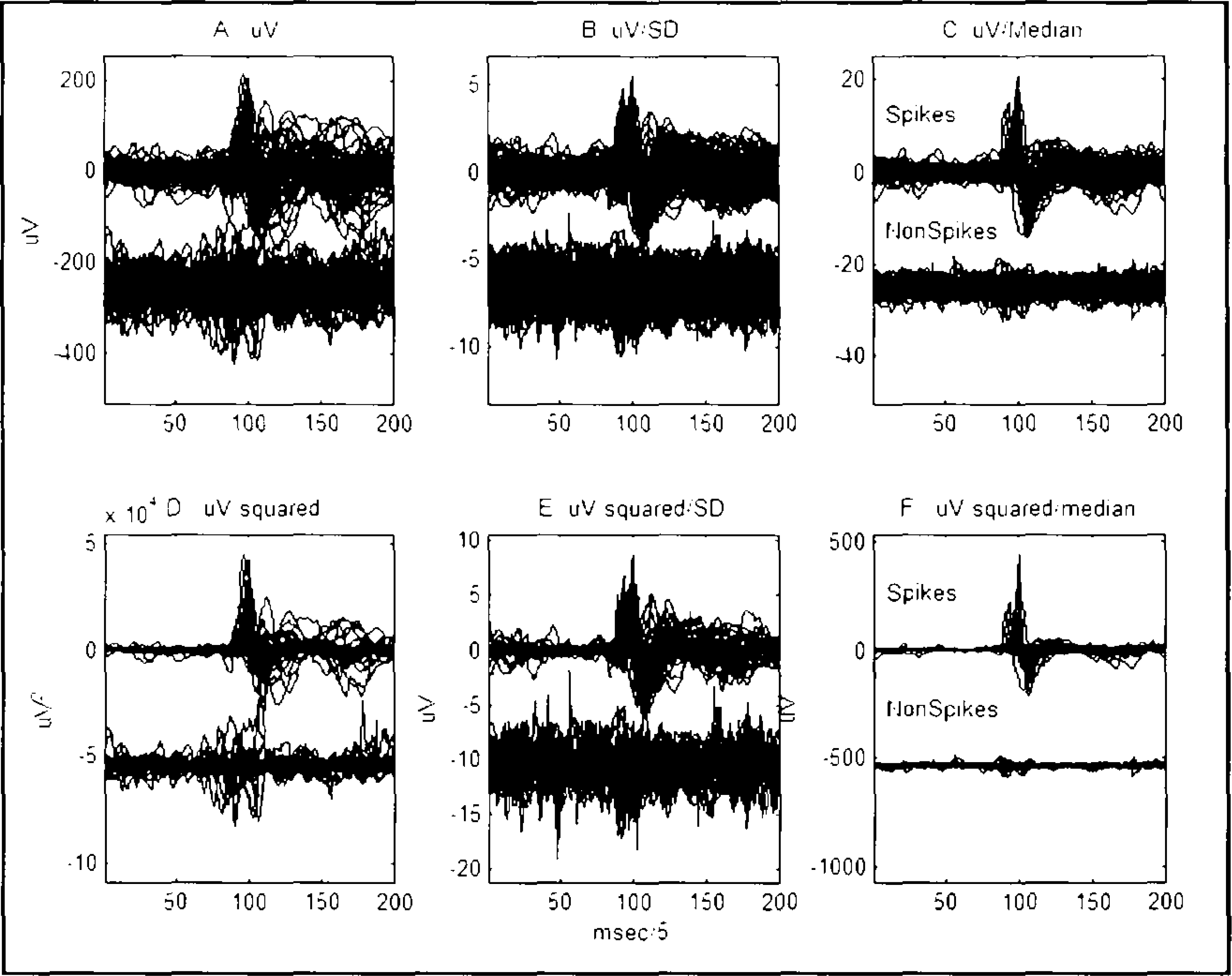
Dawson plots of superimposed 100 Spike and 100 NonSpike epochs. Same data as Figure 2. A-F show the comparative effects of squaring and scaling the epochs. Median scaling of amplitude (C and F) increases the Spike-NonSpike differences, especial if the sampled have been square (F, squared/median).
The data in Figure 3 is the same data as Figure 2 scaled is six different fashions. Figure 3a shows the unsealed data. Note the improved visualization of Spike samples compared to NonSpike samples, when scaling by the median as compared to the SD is used, as seen in Figure 3b-c.
Nonlinear transformations to enhance spike activity have been suggested for AESD, such as the square root, first derivative, square and most recently NLEO. NLEO, enhances high amplitude fast activity, muscle activity more that spike activity. However, simply squaring each the samples, maintaining the sign work better for spike activity (Figure 3d-e). Further enhance of the difference between spike and background activity can be obtained by dividing the squared signed samples by the local median of all 200 values in the epoch (Figure 3f).
Amplitude and duration parameters
We use a small Matlab® program to detect all EEG peaks and calculate the interpeak amplitudes and durations. Interpeak parameters are better for spike detection than zero-crossing parameters because (1) more of the waveform is retained and no spikes are missed, (2) slower activity is de-emphasized and (3) spike amplitudes and durations are more widely separated from background faster rhythms.
Figure 4 shows the A-D distribution of individual waves in spike and nonspike epochs, without (4a) and without (4b) squared/median scaling of amplitudes. Note the tight clustering of Spike maxima.
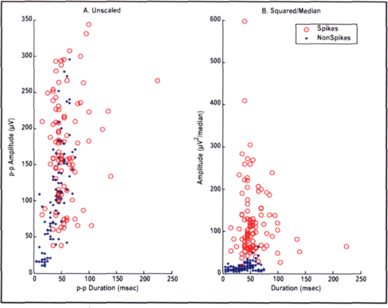
Amplitude vs Duration Scatterplot of 100 Spike and 100 NonSpike epoch maxima. A, no scaling. B, squared/median scaling, as in Figure 3f. Maxima are consistent indicators of spike peaks after appropriate scaling.
Figure 5 shows the spike detection results when a threshold of 25 times the median p-p squared amplitude in an epoch is exceeded. Same data as Figures 3f and 4b. Detections of Spikes and false positive detections of nonspikes are shown in red. Sensitivity is 90%, specificity 92% and PPV 91%, a respectable range. Squared/median-scaled peak-peak amplitude is a powerful parameter for spike detection that can be used as a benchmark for evaluating other candidate detection parameters. More importantly, we can examine the individual spikes that were missed and the false positives that were detected and use this visual information of EDS to formulate plans for changing thresholds, 96 adding parameters, and developing advanced classification methods 76,78–79 –82 –93 This is the major advantage of the scatterplots, Dawson plots, and thumbnail plots used in EDA: the ability to retain a balance of individual and synoptic information enhance the evaluation of group differences and similarities.
SUMMARY
Since the 1970s advances in science and technology during each succeeding decade have renewed the expectation of efficient, reliable automatic epileptiform spike detection (AESD). But even when reinforced with better, faster tools, clinically reliable unsupervised spike detection remains beyond our reach.
Expert-selected spike parameters were the first and still most widely used for AESD. Thresholds for amplitude, duration, sharpness, rise-time, fall-time, after-coming slow waves, background frequency, and more have been used. It is still unclear which of these wave parameters are essential, beyond peak-peak amplitude and duration. Wavelet parameters are very appropriate to AESD but need to be combined with other parameters to achieve desired levels of spike detection efficiency.
Artificial Neural Network (ANN) and expert-system methods may have reached peak efficiency. Support Vector Machine (SVM) technology focuses on outliers rather than centroids of spike and nonspike data clusters and should improve AESD efficiency.
An exemplary spike/nonspike database is suggested as a tool for assessing parameters and methods for AESD and is available from the author at
Exploratory Data Analysis (EDA) is presented as a graphic method for finding better spike parameters and for the step-wise evaluation of the spike detection process.
DISCLOSURE AND CONFLICT OF INTEREST
R. Harner has no conflicts of interest in relation to this article.