Investigations on Multiple Protein Scaffold Filling

Abstract

In this article, we initiate the study on some problems related to multiple protein scaffold filling, with or without references. The objective is to maximize the sum of Blosum62 scores of the filled sequences when no reference is given, or to maximize the Blosum62 score between the filled sequence and a reference. We present the following results: (1) given n scaffolds generated from the top-down tandem mass spectra, finding k scaffolds whose corresponding contents can be used to fill into a target sequence (or a sequence whose Blosum62 score with a reference is maximized) takes $Ω (n^{k - ε})$ time, unless the Strong Exponential Time Hypothesis (SETH) fails. (2) Given two or more protein scaffolds and the corresponding multisets of amino acids to be filled accordingly, the corresponding optimization problem can be solved in polynomial time with dynamic programming. (3) Due to the high (and impractical) running times of these algorithms, we implement several heuristic algorithms for the special cases when three scaffolds are given. The corresponding empirical results are quite promising, from the testing of 12 datasets spanning five different kinds of proteins: antibody, myoglobin, mitochondrial respiratory-chain, calmodulin, and thioredoxin.

Keywords

colinear chaining greedy algorithms lower bound protein scaffold filling protein sequencing top-down and bottom-up methods simulated annealing

1. INTRODUCTION

Protein sequencing is a fundamental problem in computational biology, as the given sequence of a protein can give us a lot of important information, like its structure, function, biomarkers, etc. Consequently, Edman tried to sequence a peptide (a short segment of protein) as early as 1949 (Edman, 1949). However, this method can only handle very small protein sequences and is error-prone. Since the 1970s, de novo protein sequencing has become dominant with bottom-up and top-down methods. The former first constructs a lot of peptides using mass spectrometry (MS), then tries to assemble them together into a sequence using a graph method; the latter can directly sequence a protein with its mass bounded by roughly 30k Daltons, but usually will leave some gaps. (For scaffolds constructed from top-down mass spectra, we usually have the extra property that the positions, sizes and/or the total weight/mass of the gaps are known.) For a complete background on de novo protein sequencing, readers are referred to (Aebersold and Mann, 2003; Liu et al., 2014; Tran et al., 2016).

However, even though these methods have been quite effective, many assembled proteins remain incomplete, with gaps in their scaffolds (Tran et al., 2016). In addition to possible errors or limitations in mass spectrometry and assembly software, certain segments remain elusive, complicating the prediction of missing amino acids within scaffold gaps (Tran et al., 2016). Hence, with either the bottom-up or top-down method, at the end, we are likely to have a broken protein sequence or scaffold: a sequence of contigs with a gap size or gap mass might or might not be known. This raises a natural question: Given a protein scaffold, how to fill those gaps?

Filling a protein scaffold with a reference was first studied by Qingge et al. (2017). The problem is defined as follows: given a protein scaffold $S_{1}$ , a complete protein sequence R as reference and a multiset $X_{1}$ of amino acids, fill the amino acids in $X_{1}$ into the gaps in $S_{1}$ to obtain $S_{1}^{'}$ such that the Blosum62 score between $S_{1}^{'}$ and R is maximized. The problem was shown to be polynomially solvable, but the running time is too high. Hence, Qingge et al. also designed several heuristic algorithms based on greedy and local search (Qingge et al., 2017). Note that usually $X_{1} = c (R) - c (S_{1})$ , but certainly it does not have to be the case.

In reality, for many proteins, such as an antibody, it is hard to find the right reference. Hence, a lot of research has recently been done based on the use of machine learning and probabilistic methods (Badal et al., 2024,2025; Qingge et al., 2025; Sturtz et al., 2022,2023). We encourage readers to review these articles for more details.

In practice, sometimes we might need to recover protein sequences with at least two chains. Or, because of mutations and post-translational modifications (PTM), a protein could result in several proteoforms that need to be recovered or sequenced. Using top-down MS tools, it is often difficult to separate these proteoforms (DiMaggio et al., 2009). In this case, a multiplexed tandem mass spectrum (MTM) is generated when tandem mass spectrometry (MS/MS) is used on two or more proteoforms that are not well separated by protein separation methods (Wang et al., 2010). Some subsequent research has used MTM to try to sequence these proteoforms (Wang et al., 2014; Zhu and Liu, 2018). Due to the complexity of MTM spectra, it is not surprising that we might only obtain a set of $ℓ$ scaffolds instead of complete sequences of $ℓ$ .

In this article, we initialize the study on the multiple protein scaffold filling problems, which certainly have several different versions based on many factors. For instance, are the scaffolds generated from top-down or bottom-up method? (The former usually contains the positions information, i.e., the positions of gaps or unknown amino acids are known; while this is not usually the case for the latter.) In addition, there could be extra constraints, such as on the amino acids to be filled. For instance, are they given as a multiset? or as several multisets corresponding to each of the given scaffolds to be filled? or even as a set of contigs or multiple sets of contigs? Constraints like these could significantly change the complexity of the problem. In this article, we report some results along the line.

This article is organized as follows. In Section 2, we give necessary definitions. In Section 3, we present a conditional lower bound on filling scaffolds generated by a top-down method. In Section 4, we briefly discuss some other solvable cases. In Section 5, we present some practical results on the version of filling three scaffolds (to maximize the sum of the corresponding Blosum62 scores between the filled sequences). We conclude the article in Section 6.

2. PRELIMINARIES

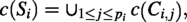
Let n be a natural number, define $[n] = {1, 2, ..., n}$ . Let $Σ$ be the set of 20 amino acids. Let $B 62 (a, b)$ be the Blosum62 score between two amino acids a and b. (The Blosum62 matrix was proposed in Henikoff and Henikoff (1992), and for completeness, we list it in the Appendix as Table A3). A protein sequence S is a sequence over $Σ$ . We denote the multiset of amino acids in S as $c (S)$ . A contig is a short protein sequence, usually obtained by some sequencing software, say, based on the peptides obtained from mass spectrometry. A protein scaffold $S_{i}$ is a sequence of $p_{i}$ contigs $C_{i, 1}, C_{i, 2}, \dots, C_{i, p_{i}}$ , with gaps $G_{i, j}$ between neighboring contigs $C_{i, j}$ and $C_{i, j + 1}$ , for $1 \leq j \leq p_{i} - 1$ , where some missing amino acids can be inserted. We define $c (S_{i})$ as

c (S_{i}) = \cup_{1 \leq j \leq p_{i}} c (C_{i, j}),

i.e., it is the multiset of amino acids appearing in all the contigs of

S_{i}

2.1. Problems

In the traditional version following (Qingge et al., 2017), given two or more protein scaffolds $S_{1}, S_{2}$ , $\dots, S_{m}$ (each $S_{i}$ has $p_{i}$ contigs, for $1 \leq i \leq m)$ and m multisets of amino acids $X_{1}, X_{2}$ $\dots, X_{m}$ , fill $X_{i}$ into the gaps in $S_{i}$ to have $S_{i}^{'}$ such that the total Blosum62 scores between $S_{i}^{'}$ and $S_{j}^{'}$ , $1 \leq i \neq j \leq m$ , is maximized; or, the sum of Blosum62 scores between $S_{i}^{'}$ and $S_{j}^{'}$ is maximized for $1 \leq i \neq j \leq m$ . A variation is that instead of given m multisets of amino acids as part of the input, we are only given a multiset X of amino acids. In both of these versions, X and $X_{i}$ ’s could be multisets of contigs (instead of amino acids).

Regarding the scaffolds generated from the top-down method (where the position and size of each gap are known), we are given a set of scaffolds $T = {T_{1}, T_{2}, ..., T_{n}}$ , a source scaffold B and a target sequence T, the question is to find k scaffolds in $T$ whose corresponding (non-gap) contents can be used to fill into B to form the target sequence T. We call this problem the k-top-down scaffold problem (k-TDS, for short). Alternatively, we are given $T$ , a source scaffold B and a reference R, the question is to search for k scaffolds in $T$ to fill B into a sequence T such that $B 62 (T, R)$ is maximized. We call this latter problem the k-top-down scaffold problem with reference.

An example of the k-top-down scaffold problem is given as follows. For simplicity, we use a small alphabet ${A, V, W, ⋆}$ , where A, V, W are amino acids and $⋆$ is a space. Let $B = AVWA ⋆ ⋆ ⋆ W VAWV ⋆ ⋆ V WAWA$ , and $T = AVWA \cdot VWA \cdot WVAWV \cdot A V \cdot VWAWA$ . Then the problem is to search in $T$ some $T_{i}$ whose non-gap contents best match VWA (T[5.7]) and some $T_{j}$ whose non-gap contents best match AV (T[13.14]), when T is viewed as an array T[1.19].

A naive algorithm is to use a k-nested loop to search for k scaffolds in $T$ , resulting a running time of $O (n^{k} \cdot | T |)$ . In the next section, we first show that this naive algorithm is in fact almost optimal — under the SETH (which states that SAT of n variables cannot be solved in $2^{(1 - ε) n}$ time, for some $ε > 0$ ).

3. A LOWER BOUND FOR THE k TOP-DOWN SCAFFOLD PROBLEM

We will use only two amino acids plus the empty symbol $⋆$ (which represents one gap) in our construction, e.g., $Σ^{'} = {⋆, A, W}$ . Let $B 62 (a, b)$ be the Blosum62 score between two amino acids a and b. (Note that $B 62 (a, b)$ is symmetric, i.e., $B 62 (a, b) = B 62 (b, a)$ .) We would use $B 62 (x, y)$ for two protein sequences x and y of the same length. It is known that

B 62 (A, A) = 4, B 62 (W, W) = 11, B 62 (A, W) = - 3,

and

B 62 (A, ⋆) = B 62 (W, ⋆) = - 4.

We comment that in many articles the gap penalty is −1, but to be consistent with our algorithm in Section 5 (using the Needleman–Wunsch [NW] algorithm), we use −4. This will not affect our proof; in fact, any negative gap penalty would work.

We prove the conditional lower bound by using an idea from (Feng et al., 2024), on the k-SUM problem over large integers. The idea in Feng et al. (2024) is a twist of Williams’ Orthogonal Vector problem (Williams, 2005). Of course, different from the ideas in (Feng et al., 2024), we need to construct protein scaffolds instead of integer vectors.

Given a SAT instance $ϕ$ with n variables and m clauses, the SETH was first posed as an open question by Impagliazzo and Paturi (Impagliazzo and Paturi, 2001): can $ϕ$ be decided to have a truth assignment in $2^{(1 - ϵ) n}$ time? SETH was named later in Calabro et al. (2009).

In Feng et al., (2024), Feng, Fernau, and Zhu used a special version of SAT, one-in-three SAT, which was also known to be NP-complete (Schaefer, 1978). Here we also use one-in-three SAT. Note that, to maintain the NP-completeness of the input instance, we need to have $m = Ω (n)$ .

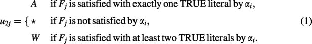
Formally, let $ϕ$ be a One-in-three SAT instance composed of n variables and m disjunctive clauses where the i-th clause $F_{i}$ contains three literals and is in the form of $(x_{i, 1} \lor x_{i, 2} \lor x_{i, 3})$ . The problem is to determine for $i = 1.. m$ , exactly one of the three literals in each clause $F_{i}$ , i.e., $x_{i, 1}, x_{i, 2}$ and $x_{i, 3}$ , is assigned TRUE.

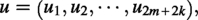
We arbitrarily partition the variables in $ϕ$ into k equal-sized parts $V_{1}, V_{2}, \dots V_{k}$ (we can assume that n is a multiple of k, though it does not really matter for the result). Each of the $2 (m + k)$ -sequences $u \in U_{i}$ is determined by an assignment $α_{i}$ of $V_{i}$ (i.e., a partial assignment of the variables in $ϕ$ ), where:

u = (u_{1}, u_{2}, \dots, u_{2 m + 2 k}),

and

u_{2 ℓ + 1} = W

for all

0 \leq ℓ \leq m + k - 1

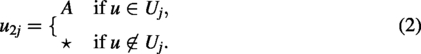
. In fact, we could think of each W as (a part of) a contig. Then, for

1 \leq j \leq m

, we construct:

u_{2 j} = {\begin{array}{l} A & if F_{j} is satisfied with exactly one TRUE literal by α_{i}, \\ ⋆ & if F_{j} is not satisfied by α_{i}, \\ W & if F_{j} is satisfied with at least two TRUE literals by α_{i} . \end{array}

(1)

For $m + 1 \leq j \leq m + k$ , we additionally construct:

u_{2 j} = {\begin{array}{l} A & if u \in U_{j}, \\ ⋆ & if u \in U_{j} . \end{array}

(2)

The source scaffold is $B = {(W ⋆)}^{m + k}$ , the target sequence is $T = {(W A)}^{m + k}$ , and the set of scaffolds are:

T = U_{1} \cup U_{2} \cup \dots \cup U_{k} .

Then, we can claim that $ϕ$ has a valid truth assignment if and only if there are k scaffolds $T_{i} \in U_{i} \subset T, i \in [k]$ , whose corresponding contents can be filled into B to obtain T. As there are $2^{n / k}$ assignments for $V_{1}, V_{2}, \dots, V_{k}$ respectively, the above reduction takes $2^{n / k} \cdot O (m + k)$ time. If k-TDS could be computed in $O (N^{k - ε})$ time, where N is the input size for k-TDS, one-in-three SAT could be solved in $2^{n - n ε / k} \cdot O ({(m + k)}^{k - ε})$ time—which would fail the SETH. We hence have the following theorem.

Theorem 1. The k-top-down scaffold problem, with input size N, cannot be solved in $O (N^{k - ϵ})$ time unless the SETH fails.

We give a simple example for the above reduction. Let the One-in-three SAT instance be:

ϕ = (x_{1} \lor x_{2} \lor x_{3}) \land (x_{1} \lor {\bar{x}}_{2} \lor x_{4}) \land (x_{2} \lor x_{3} \lor {\bar{x}}_{4}) \land (x_{1} \lor {\bar{x}}_{3} \lor {\bar{x}}_{4}) .

Then $n = 4$ and $m = 4$ ; and a valid truth assignment is $x_{1} = FALSE$ , $x_{2} = TRUE$ , $x_{3} = FALSE$ and $x_{4} = TRUE$ .

By construction,

B = {(W ⋆)}^{m + k} = W ⋆ \cdot W ⋆ \cdot W ⋆ \cdot W ⋆ \cdot W ⋆ \cdot W ⋆,

and the target sequence is

T = {(W A)}^{m + k} = W A \cdot W A \cdot W A \cdot W A \cdot W A \cdot W A .

Suppose that $k = 2$ and we partition the variables into $V_{1} = {x_{1}, x_{2}}$ and $V_{2} = {x_{3}, x_{4}}$ . Corresponding to the partial assignment $x_{1} = FALSE$ and $x_{2} = TRUE$ , the corresponding sequence constructed in $U_{1}$ is:

T_{1} = W A \cdot W ⋆ \cdot W A \cdot W ⋆ \cdot W A \cdot W ⋆ .

Due to space constraint, we ignore the other 3 sequences in $U_{1}$ . Similarly, corresponding to the partial assignment for variables in $V_{2}$ , i.e., $x_{3} = FALSE$ and $x_{4} = TRUE$ , the corresponding sequence in $U_{2}$ is

T_{2} = W ⋆ \cdot W A \cdot W ⋆ \cdot W A \cdot W ⋆ \cdot W A .

Note that $T = U_{1} \cup U_{2} = {T_{1}, T_{2}, \dots, T_{8}}$ , and the problem is to search for $T_{1}$ and $T_{2}$ in $T$ to fill the corresponding contents to B to be equal to T. More specifically, we need to fill the A’s at position 2, 6, and 10 from $T_{1}$ , and at position 4, 8, and 12 from $T_{2}$ , into the corresponding $⋆$ positions in B.

Corollary 1. The k-top-down scaffold problem with reference, with input size N, cannot be solved in $O (N^{k - ϵ})$ time unless the SETH fails.

Proof. We just set $R = T = {(W A)}^{m + k}$ . Then the Blosum62 score to optimize is $B 62 (T, R) = 11 (m + k) + 4 (m + k) = 15 (m + k)$ .▪

4. SOLVABLE CASES IN THE TRADITIONAL MODEL

In this section, we briefly mention some solvable cases in the traditional model. In fact, as the running times of these algorithms are so high, it is not practical to really implement them. Hence, these results are only theoretically meaningful. As a matter of fact, here we focus on the number of matched pairs in the solution rather than the Blosum62 scores. This can be done by rounding the Blosum62 matrix as follows: if a cell has a value $\geq 4$ , then change it to 1; otherwise, change it to 0. Since the gap penalty is $- 4$ , we could just disallow gaps and assume that the filled solutions (without gaps) all have the same length.

4.1. Two or three scaffolds, no reference

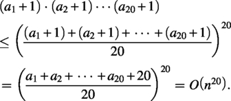
First, note that given a set X of n amino acids, the total subsets of X is bounded by $O (n^{20})$ . Let $a_{i}$ be the number of i-th amino acid in X. The number of subsets of X is bounded by:

\begin{array}{l} (a_{1} + 1) \cdot (a_{2} + 1) \dots (a_{20} + 1) \\ \leq {(\frac{(a_{1} + 1) + (a_{2} + 1) + \dots + (a_{20} + 1)}{20})}^{20} \\ \begin{array}{l} = {(\frac{a_{1} + a_{2} + \dots + a_{20} + 20}{20})}^{20} = O (n^{20}) . \end{array} \end{array}

As a warm-up, we first illustrate the idea for $m = 2$ , where the input is two scaffolds $S_{1}$ and $S_{2}$ composed of contigs together with $X_{1}$ and $X_{2}$ to be inserted in $S_{1}$ and $S_{2}$ respectively. It is easy to see that, if in the optimal solution there are matches between the amino acids in $X_{1}$ and $X_{2}$ inserted in the final solution $S_{1}^{'}$ and $S_{2}^{'}$ , then we could move all these amino acids (letters) at the end of $S_{1}^{'}$ and $S_{2}^{'}$ . Hence, it suffices to discuss the cases when contigs from $S_{1}$ and $S_{2}$ having intersections.

We define $T_{1} [i, j, k, X_{1} [i, j, k]]$ as the maximum number of matched pairs obtained when the last element in contig $C_{1, i}$ is matched with the k-th letter of contig $C_{2, j}$ using the subset of amino acids $X_{1} [i, j, k]$ left from $X_{1}$ so far. Similarly, we define $T_{2} [i, j, ℓ, X_{2} [i, j, ℓ]]$ as the maximum number of matched pairs obtained when the last element in contig $C_{2, j}$ is matched with the $ℓ$ -th letter of $C_{1, i}$ using the subset of amino acids $X_{2} [i, j, ℓ]$ left from $X_{2}$ so far. The update is not hard but tedious: roughly we would pick what we have in $X_{1} [-]$ or $X_{2} [-]$ to form as many match pairs as possible and then update $X_{1} [-]$ and $X_{2} [-]$ accordingly. We ignore further details. Certainly, the final solution is to take the maximum of values in the $T_{1} [-], T_{2} [-]$ tables. Since the number of subsets of each of $X_{1}$ and $X_{2}$ is $O (n^{20})$ , the cost would be high. We summarize the result as an observation.

Observation 1. The two-scaffold filling problem can be solved in $O (n^{44})$ time, where n is the input size.

With $m = 3$ scaffolds $S_{1}, S_{2}, S_{3}$ and the three multisets of amino acids $X_{1}, X_{2}, X_{3}$ to be inserted respectively, the cases are even more complex and tedious. With a similar argument to the case of $m = 2$ , we only need to consider 7 cases when some contigs are involved: (1) One case when three contigs from different $S_{i}$ ’s overlap, (2) Three cases when two contigs from different $S_{i}$ ’s overlap, and (3) Three cases when one contig from some $S_{i}$ (say $S_{1}$ ) is fixed and some letters from $X_{2}$ and $X_{3}$ are selected to match with this contig. The details are even more tedious, and it is not worth the effort to describe details (as the algorithm would be completely impractical). The running time of this algorithm, should be close to $O (n^{66})$ , where n is the total input size of the problem.

4.2. Other solvable cases

For some other cases, we can show that the problem of filling d scaffolds with one reference, and filling one scaffold with d references are both polynomially solvable when d is fixed. But, as the running time is large (at least $Ω (n^{20 d}$ ), these algorithms are also impractical. Hence, we do not give further details.

In the next section, we consider designing and implementing some practical algorithms. We choose the problem of filling three scaffolds in the traditional model, that is, given three scaffolds $S_{1}, S_{2}, S_{3}$ and also three sets $X_{1}, X_{2}, X_{3}$ , to be filled in the scaffolds accordingly. The objective is to maximize the sum of Blosum62 scores between the filled sequences $S_{1}^{'}, S_{2}^{'}$ and $S_{3}^{'}$ .

5. PRACTICAL ALGORITHMS FOR FILLING THREE SCAFFOLDS

In this section, we study scaffold gap filling with multiple protein scaffolds. Specifically, we focus on three protein scaffolds. These methods should be easily generalized to more than three (say five) protein scaffolds, although the running time would certainly be higher.

5.1. Problem setting and motivation

Given three incomplete but homologous scaffolds $I = {I_{1}, I_{2}, I_{3}}$ containing unknown residues (denoted by *), and for each gap, a small admissible set of residues or short fragments to choose from, the goal is to reconstruct complete sequences $S_{1}^{'}, S_{2}^{'}, S_{3}^{'}$ that agrees as much as possible with a single trusted reference (ground truth) sequence $S^{⋆}$ while keeping computation tractable.

5.1.1. Notation

Each scaffold $I_{ℓ}$ ( $ℓ \in {1, 2, 3}$ ) is a string over the amino-acid alphabet $Σ$ augmented with a special gap symbol *. Let $G_{ℓ} = {g_{ℓ, 1}, \dots, g_{ℓ, m_{ℓ}}}$ index gap positions in $I_{ℓ}$ . At gap $g_{ℓ, j}$ , we allow a candidate set $X_{ℓ, j} \subseteq Σ$ (single residues) or, more generally, a small set of short fragments $X_{ℓ, j} \subseteq Σ^{\leq k}$ . Filling all gaps in $I_{ℓ}$ with choices from $X_{ℓ, j}$ yields a complete sequence $S_{ℓ}^{'} \in Σ^{n_{ℓ}}$ . Throughout, we use BLOSUM62 and a linear gap penalty $γ = - 4$ .

5.1.2. Scoring objectives

We use NW for global alignment. Because the three scaffolds are homologous views of the same domain, we aggregate pairwise agreement in two ways:

Truth-referenced objective:

F_{truth} (S_{1}^{'}, S_{2}^{'}, S_{3}^{'}) = NW (S_{1}^{'}, S^{⋆}) + NW (S_{2}^{'}, S^{⋆}) + NW (S_{3}^{'}, S^{⋆}) .

(3)

Triple agreement objective:

F_{triple} (S_{1}^{'}, S_{2}^{'}, S_{3}^{'}) = NW (S_{1}^{'}, S_{2}^{'}) + NW (S_{2}^{'}, S_{3}^{'}) + NW (S_{1}^{'}, S_{3}^{'}) .

(4)

5.1.3. Truth constant

With a single reference $S^{⋆}$ shared by all three scaffolds, the maximum of (3) is achieved when $S_{1}^{'} = S_{2}^{'} = S_{3}^{'} = S^{⋆}$ , hence

TRUTH \overset{def}{=} \max_{S_{1}^{'}, S_{2}^{'}, S_{3}^{'}} F_{truth} (S_{1}^{'}, S_{2}^{'}, S_{3}^{'}) = 3 \cdot NW (S^{⋆}, S^{⋆}) .

For each data set, we therefore report the achieved scores (Greedy, SA) along with Truth and the gaps to optimality Δ_Greedy = Greedy − Truth and Δ_SA = SA − Truth.

5.1.4. Computational difficulty

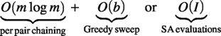
Optimizing (4) or (3) in combinatorial space $\prod_{ℓ, j} X_{ℓ, j}$ is intractable in the worst case. Each evaluation requires three NW alignments ( $O (n^{2})$ DP per pair), and the search space grows exponentially with the number of gaps and candidates. This motivates heuristics that (i) reduce the search space and (ii) bias exploration toward promising regions.

5.1.5. Algorithmic families

We evaluated three families of methods:

Greedy (baseline). Visit the gaps in fixed order. For each gap, try all admissible candidates and commit the best choice locally under (4) while holding previous decisions fixed. Very fast, but can get trapped in local optima.

Simulated annealing (SA, baseline). Start from Greedy (or a random fill). Perform stochastic local moves (mutating one or two gaps); accept improvements or, with probability $\exp (Δ / T)$ , occasional degradations while cooling temperature T. Improves quality at higher cost.

Collinear chaining (our acceleration). Compute anchors (shared k-mers) between scaffold pairs; solve a collinear chaining problem to obtain ordered, nonoverlapping blocks; then restrict Greedy/SA mutations to positions within or near these blocks. During search, we use a fast block-sum proxy of (4); final scores are always recomputed with full NW. This substantially reduces run-time with minimal loss in accuracy.

5.1.6. Assumptions and practical choices

We assume (i) homologous scaffolds with partially overlapping conserved regions; (ii) small candidate sets $X_{ℓ, j}$ (single residues or short fragments) derived from plausible biochemical contexts; and (iii) BLOSUM62 with linear gaps adequately captures substitution tendencies for these datasets. These choices keep comparisons fair for all methods.

5.1.7. Evaluation goals

We address two questions:

1.
Accuracy. How close do Greedy and SA, with and without chaining, reach the upper bound Truth across datasets?
2.
Efficiency. How much wall clock time does collinear chaining save relative to baselines, and what speed-ups (mean/median) are observed?

Consequently, we report (i) the scores of the per-dataset method and $Δ$ to Truth; (ii) the runtimes of the per-dataset decomposed by phase (Greedy, SA, chain build) and totals; and (iii) mean/median speedups.
5.1.8. Working hypotheses

H1 (Accuracy):
SA typically outperforms Greedy; chaining preserves or slightly improves quality by guiding search into coherent blocks.
H2 (Efficiency):
Chaining-aware search yields large speedups (often an order of magnitude) by shrinking the neighborhood and enabling fast score updates.
5.2. Methods

5.2.1. NW (baseline alignment)

5.2.1.1. Setup

Given two sequences $A = a_{1} \dots a_{n}$ and $B = b_{1} \dots b_{m}$ , a substitution score $s (\cdot, \cdot)$ (BLOSUM62 in our experiments) and a linear gap penalty $γ = - 4$ , the NW algorithm computes a global alignment and its optimal score (Needleman and Wunsch, 1970). We maintain a dynamic programming (DP) table $D \in R^{(n + 1) \times (m + 1)}$ with the following initialization and recurrence:

\begin{array}{l} D (0, 0) = 0, D (i, 0) = i γ, D (0, j) = j γ, \\ D (i, j) = \max {D (i - 1, j - 1) + s (a_{i}, b_{j}), D (i - 1, j) + γ, D (i, j - 1) + γ}, \end{array}

(5)

for

1 \leq i \leq n

1 \leq j \leq m

. The optimal global alignment score is

NW (A, B) = D (n, m)

; a standard traceback from

(n, m)

(0, 0)

recovers one optimal alignment.

5.2.1.2. Complexity

The DP fills $(n + 1) (m + 1)$ cells and each cell performs $O (1)$ work, so the time complexity is $O (n m)$ and the memory footprint is $O (n m)$ . When only the score is needed, memory can be reduced to $O (\min {n, m})$ by keeping two rows; when the alignment itself is required, Hirschberg’s divide–and–conquer variant achieves $O (n m)$ time and $O (n + m)$ memory.

5.2.1.3. Use in our pipeline

NW is the scoring oracle throughout our experiments. (i) To evaluate reconstructed scaffolds, we use the triple agreement objective $F_{triple}$ defined in equation (4). (ii) When a trusted reference $S^{⋆}$ is available, we also report the truth-referenced objective $F_{truth}$ from equation (3); its maximum is the constant Truth. All heuristic search procedures (Greedy, SA, and their chaining-aware variants) ultimately validate their solutions by recomputing these objectives with full NW.

5.2.1.4. Practical notes

Our sequences are antibody light chains (hundreds of residues), for which the $O (n m)$ memory is acceptable; thus, we use a full DP table to enable fast traceback. For accelerations, we optionally employ (banded NW) in intermediate steps, but all reported scores use the exact global NW with BLOSUM62 and $γ = - 4$ .

5.2.2. Greedy heuristic

5.2.2.1. Idea

Greedy fills the gaps one by one. Fix an ordering of all gap locations $G = {g_{1}, \dots, g_{M}}$ across the three scaffolds. For the t-th gap $g_{t}$ (belonging to some scaffold $I_{ℓ}$ ), we try every admissible candidate $x \in X_{g_{t}}$ , temporarily substitute x at that position, score the resulting partial sequences using the search objective $F_{triple}$ in (4), and keep the best-scoring choice. Earlier decisions are held fixed; the process repeats until all gaps are filled.

5.2.2.2. Pseudo-code

Let $S_{1}^{'}, S_{2}^{'}, S_{3}^{'}$ be the current (partially filled) sequences.

1.
Initialize $S_{ℓ}^{'} \leftarrow I_{ℓ}$ for $ℓ \in {1, 2, 3}$ .
2.
For $t = 1$ to M: a.
For each $x \in X_{g_{t}}$ , set $S_{ℓ}^{'} [g_{t}] \leftarrow x$ (others unchanged), compute $v_{x} = F_{triple} (S_{1}^{'}, S_{2}^{'}, S_{3}^{'})$ .
b.
Select $x^{⋆} = \arg \max_{x} v_{x}$ and commit $S_{ℓ}^{'} [g_{t}] \leftarrow x^{⋆}$ .

3.
Return $S_{1}^{'}, S_{2}^{'}, S_{3}^{'}$ and their scores (and later report $F_{truth}$ ).

5.2.2.3. Complexity

Let $K_{t} = | X_{g_{t}} |$ be the number of admissible choices at gap $g_{t}$ , and let $C_{eval}$ be the cost of one objective evaluation. In the naive implementation (recomputing full NW scores each time), $C_{eval} = O (n^{2})$ for sequence length n (three pairwise DPs), and the total time is:

T_{greedy} = O ((\sum_{t = 1}^{M} K_{t}) C_{eval}) = O ((\sum_{t = 1}^{M} K_{t}) n^{2}) .

When each gap offers a bounded alphabet-sized set $K_{t} \approx k$ and the effective gap length being optimized is $n_{g}$ , this is often summarized as $O (n_{g} k)$ evaluations. In our code, we use exact NW for reporting, so wall-clock scales with the number of Greedy evaluations times the DP cost. (Section 5.2.4 shows how chaining greatly reduces the number of evaluated positions.)

5.2.2.4. Strengths and limitations

Greedy is extremely fast and simple, and provides strong initial solutions that SA can refine. However, because each choice is committed irrevocably, the method is sensitive to local optima and may miss globally better combinations of gap fills—particularly when interacting choices span multiple neighboring gaps.

5.2.3. Simulated annealing

5.2.3.1. Idea

SA is a stochastic local search that explores a neighborhood of solutions by applying small random mutations to the current sequences. Depending on the experimental configuration, SA may start either from a random initialization or from the Greedy fill. SA accepts any improving move and, with probability $\exp (Δ / T)$ , also accepts a worsening move of score change $Δ < 0$ at temperature T. As T is gradually cooled, the algorithm becomes more conservative, helping it escape local optima early and refine later.

5.2.3.2. Neighborhood

At each iteration, we randomly choose either (i) a single-site move: pick one gap position g and replace its current residue/fragment by another candidate from $X_{g}$ , or (ii) a two-site move: mutate two gaps jointly. Joint moves help traverse interacting choices across nearby gaps. Scoring uses the search objective $F_{triple}$ in (4); final reporting uses $F_{truth}$ .

5.2.3.3. Pseudo-code

Let $S^{'} = (S_{1}^{'}, S_{2}^{'}, S_{3}^{'})$ be the current solution initialized by Greedy.

1.
Set $T \leftarrow T_{0}$ (initial temperature). Evaluate $f = F_{triple} (S^{'})$ .
2.
For $t = 1$ to max_iter: (a)
Sample a mutation (one-site w.p. $1 - p$ , two-site w.p. p) to obtain $S^{cand}$ .
(b)
Compute $f^{cand} = F_{triple} (S^{cand})$ and $Δ = f^{cand} - f$ .
(c)
If $Δ \geq 0$ , accept: $S^{'} \leftarrow S^{cand}, f \leftarrow f^{cand}$ . Else accept with probability $\exp (Δ / T)$ .
(d)
Cool: $T \leftarrow α T$ with cooling rate $α \in (0, 1)$ .
(e)
Track the best state $S^{}$ seen so far (by f).

3.
Return $S^{}$ (then compute $F_{truth}$ for reporting).

5.2.3.4. Acceptance rule and schedule

The Metropolis acceptance $\Pr [accept] = \exp (Δ / T)$ for $Δ < 0$ enables occasional uphill (worse) moves when T is high, helping the search escape local optima. We use geometric cooling $T_{t + 1} = α T_{t}$ with $α \in [0.98, 0.999]$ depending on the run budget, multiple short restarts are optional.

5.2.3.5. Complexity

Let I be the number of iterations and let $C_{eval}$ be the cost of one objective evaluation (three NW alignments in the naive form, $C_{eval} = O (n^{2})$ for sequence length n). The total time is:

T_{SA} = O (I C_{eval}) .

Equivalently, with neighborhood size summarized by an effective number of candidate mutations per iteration b (often $b \approx 1$ because we sample a single mutation), SA performs $O (I)$ evaluations, so wall-clock is proportional to I times the DP cost. Compared with Greedy, SA is typically slower but achieves higher scores by escaping local optima.

5.2.3.6. Strengths and limitations

SA provides a principled mechanism to balance exploration and exploitation and consistently improves over Greedy in our experiments. Its drawbacks are higher runtime and sensitivity to schedule parameters $(T_{0}, α, I)$ ; we mitigate the latter by initializing from Greedy and using conservative cooling with a small probability of two-site moves.

5.2.4. Collinear chaining

5.2.4.1. Idea

To shrink the search space, we identify anchors—short exact matches (common k-mers) between pairs of scaffolds—and compute a maximum‐weight collinear chain of anchors that are consistent in order. Chained anchors are then inflated into blocks (conserved regions), and Greedy/SA mutations are restricted to gaps that lie inside or near these blocks. Related practical improvements to colinear chaining have been reported in the literature (Rizzo et al., 2025). During search we evaluate a fast block‐sum proxy; final scores are recomputed with full NW to preserve correctness.

5.2.4.2. Pairwise anchors

For two strings U, V, an anchor is a triple $a = (i, j, ℓ)$ meaning $U [i : i + ℓ - 1] = V [j : j + ℓ - 1]$ with $ℓ \geq k$ . We collect anchors by hashing k‐mers (linear time in practice). Let $A = {a_{1}, \dots, a_{m}}$ be all anchors with weights $w (a) = ℓ$ (or a log‐scaled variant).

5.2.4.3. Collinear chain DP

Two anchors $a = (i, j, ℓ)$ and $b = (i^{'}, j^{'}, ℓ^{'})$ are compatible if $i + ℓ \leq i^{'} + δ$ and $j + ℓ \leq j^{'} + δ$ (nonoverlapping, allowing a small slack $δ$ ). The maximum‐weight chain solves

\max_{C \subseteq A chain} \sum_{a \in C} w (a), with DP best (b) = w (b) + \max_{a ≺ b} best (a),

where

a ≺ b

denotes compatibility and increasing order in both coordinates. With anchors sorted by

(i, j)

, we compute

best (\cdot)

O (m \log m)

using a Fenwick/segment tree keyed by j (LIS‐style speed‐up). Thus, for each pair

(I_{ℓ}, I_{ℓ^{'}})

the chaining cost is

T_{chain} = O (m \log m) after O (n_{ℓ} + n_{ℓ^{'}}) anchor  extraction .

5.2.4.4. Blocks and consensus

Chained anchors are inflated into disjoint blocks by merging adjacent anchors and padding each side by a small constant p to absorb minor indels. For three scaffolds $(I_{1}, I_{2}, I_{3})$ , we run chaining for pairs (1,2), (2,3), (1,3), and project the resulting pairwise blocks back to per‐sequence block masks $B_{1}, B_{2}, B_{3}$ . The consensus search region is the union of block masks per sequence; only gaps falling inside these masks (or within p of a mask) are considered mutable.

5.2.4.5. Block‐sum proxy for fast scoring

Let B range over blocks, and let $S^{'} = (S_{1}^{'}, S_{2}^{'}, S_{3}^{'})$ be the current fill. Instead of re‐aligning the full strings at every mutation, we maintain

{\hat{F}}_{triple} (S^{'}) = \sum_{B} [NW (S_{1}^{'} [B], S_{2}^{'} [B]) + NW (S_{2}^{'} [B], S_{3}^{'} [B]) + NW (S_{1}^{'} [B], S_{3}^{'} [B])],

which supports

O (1)

block updates after a local mutation (only the blocks touching the edited gap are recomputed). The final reported score is always the full objective (

F_{triple}

for selection;

F_{truth}

for reporting).

5.2.4.6. Integration into greedy and SA

Greedy + Chaining. Iterate over gaps restricted to the consensus masks; for each candidate, update only the affected blocks and pick the best local improvement under ${\hat{F}}_{triple}$ .

SA + Chaining. Use the same restricted neighborhood (one‐site or two‐site mutations inside/near blocks) and evaluate proposals with the block‐sum proxy; apply the usual Metropolis rule and cool the temperature.

This reduces the effective neighborhood size from n potential sites to $b ≪ n$ block‐constrained sites and replaces full realignments by small block updates.

5.2.4.7. Complexity and speed

Let b be the number of mutable gaps inside/near blocks and I the number of SA iterations. Then

\underset{per pair chaining}{\underset{︸}{O (m \log m)}} + \underset{Greedy sweep}{\underset{︸}{O (b)}} or \underset{SA evaluations}{\underset{︸}{O (I)}}

dominates the refinement phase, since each proposal touches

O (1)

blocks. Empirically,

b ≪ n

and block updates are short, yielding order‐of‐magnitude wall‐clock reductions while preserving accuracy.

5.2.4.8. Practical notes

We use exact k‐mer anchors ( $k \in [3, 5]$ ), enforce uniqueness when possible, allow small overlaps ( $δ, p$ ), and always verify the final solution with full NW before reporting Truth‐referenced scores.

Cost. Chaining over m anchors per pair is $O (m \log m)$ ; thereafter, each Greedy sweep or SA mutation touches $O (1)$ blocks, making score updates $O (1)$ per move and cutting the practical search cost from $O (n)$ to $O (b) (b ≪ n)$ .

5.3. Experimental setup

5.3.1. Datasets

We evaluate our methods on 12 scaffold datasets derived from real protein sequences obtained from UniProt, spanning multiple protein families and species. Each dataset contains three incomplete but homologous scaffolds $(I_{1}, I_{2}, I_{3})$ with known gap positions (marked ‘*’) and a single trusted reference sequence $S^{⋆}$ used for evaluation.

The datasets cover diverse protein families, including antibody/proteoform-related sequences (Datasets 1–4), myoglobin (Datasets 5–6), mitochondrial respiratory-chain proteins (Datasets 7–9), calmodulin (Datasets 10–11), and thioredoxin (Dataset 12). This diversity allows us to evaluate robustness across different sequence structures and evolutionary contexts.

For reporting, we define the Truth upper bound as Truth = 3 · NW $(S^{⋆}, S^{⋆})$ (Sec. 5.1) and compute per-method deltas relative to Truth.

5.3.2. Fragments/candidate sets

For each gap location we provide a small candidate set $X_{ℓ, j}$ of plausible fills (single residues or short subsequences), derived from conserved motifs or closely related chains. All methods (baseline and chained) draw exclusively from the same candidate sets to ensure a fair comparison.

5.3.3. Hardware and software

Experiments were conducted on a MacBook Pro (Apple M1, 8 GB RAM) using Python 3.13.1. Runtime is reported as wall-clock time measured with time.perf_counter().

5.3.4. Initialization and randomness

Greedy constructs an initial solution by visiting gaps in a fixed order. Baseline SA starts from a random initialization, while the chained SA variant is initialized from the Greedy solution. Both SA variants perform stochastic local moves (one-site or two-site mutations), and we fix the random seed (seed = 1234) for reproducibility.

For the chaining variants, we first construct pairwise anchor sets and collinear chains, which are then expanded into blocks (with padding $\pm 2$ residues). Mutations are restricted to gap positions within or near these blocks.

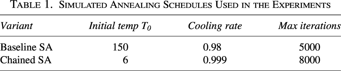
5.3.5. Hyperparameters

We use distinct SA schedules for the baseline and chained variants. Baseline SA operates over an unconstrained search space and therefore requires a higher initial temperature, while the chained variant benefits from a lower temperature and longer schedule over a restricted neighborhood. Table 1 summarizes the values used in all reported results.

Table 1.
Simulated Annealing Schedules Used in the Experiments

Variant Initial temp $T_{0}$ Cooling rate Max iterations

Baseline SA 150 0.98 5000

Chained SA 6 0.999 8000

Variant	Initial temp $T_{0}$	Cooling rate	Max iterations
Baseline SA	150	0.98	5000
Chained SA	6	0.999	8000

5.3.6. Chaining configuration

Anchors are exact k-mers with $k \in {3, 4, 5}$ (default $k = 4$ ), filtered for uniqueness when available; compatible anchors are chained with a small overlap tolerance, then merged and padded by $p = 2$ . We construct blocks for pairs $(I_{1}, I_{2})$ , $(I_{2}, I_{3})$ , and $(I_{1}, I_{3})$ and project them into per-sequence consensus masks (Section 5.2.4).

5.3.7. Outputs recorded

For each dataset and method, we report: (i) scores for Greedy and SA (both baseline and chained variants) under the Truth-referenced objective $F_{truth}$ ; (ii) the Truth constant; (iii) the corresponding gaps $Δ$ to Truth; and (iv) runtime breakdowns for Greedy, SA, chaining build, and total execution time. We also summarize mean and median speedups (baseline vs. chained) across all 12 datasets.

5.4. Results

5.4.1. Dataset structure

We evaluate on 12 scaffold datasets spanning multiple protein families (Section 5.3). Each dataset consists of three incomplete homologous scaffolds with gap positions and a single reference sequence $S^{⋆}$ used for evaluation. All results in this section are reported with respect to this reference, i.e., each method is evaluated based on how closely the reconstructed sequences match $S^{⋆}$ .

5.4.2. Scoring

All scores use NW (BLOSUM62, $γ = - 4$ ). We evaluate candidates with the truth–referenced objective $F_{truth}$ introduced in Sec. 5.1 [Eq. (3)], and compare method scores to the dataset-specific upper bound Truth. In the tables below, we report the achieved scores for all methods (Greedy, SA, and their chained variants) together with their gaps to the upper bound, Δ = score − Truth (more negative values indicate a larger deviation from the bound).

For search, we use the triple agreement objective $F_{triple}$ [Eq. (4)], while all reported numbers are recomputed using full NW scoring against $S^{⋆}$ for comparability.

5.4.3. Table overview

Tables report accuracy and runtime results across datasets. Accuracy is presented as absolute alignment scores together with their gaps to the dataset-specific upper bound Truth, while runtime is reported in seconds. Where applicable, figures provide visual comparisons of performance trends across methods and datasets.

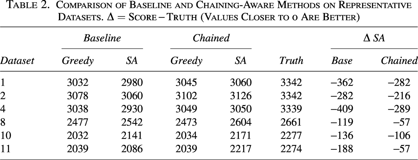
5.4.4. Accuracy

Across the representative datasets (Table 2), chaining generally moves solutions closer to the single–reference upper bound Truth. For the Greedy method, the mean gap improves modestly from ${\bar{Δ}}_{Greedy}^{base} \approx - 256.5$ to ${\bar{Δ}}_{Greedy}^{chain} \approx - 248.8$ ( $\approx + 7.7$ points). In contrast, SA benefits substantially more: the mean gap improves from ${\bar{Δ}}_{SA}^{base} \approx - 249.3$ to ${\bar{Δ}}_{SA}^{chain} \approx - 167.8$ ( $\approx + 81.5$ points).

Table 2.
Comparison of Baseline and Chaining-Aware Methods on Representative Datasets. $Δ = Score - Truth$ (Values Closer to 0 Are Better)

Dataset Baseline Chained Truth $Δ$ SA

Greedy SA Greedy SA Base Chained

1 3032 2980 3045 3060 3342 −362 −282

2 3078 3060 3102 3126 3342 −282 −216

4 3038 2930 3049 3050 3339 −409 −289

8 2477 2542 2473 2604 2661 −119 −57

10 2032 2141 2034 2171 2277 −136 −106

11 2039 2086 2039 2217 2274 −188 −57

Dataset	Baseline	Chained	Truth	$Δ$ SA
1	3032	2980	3045	3060	3342	−362	−282
2	3078	3060	3102	3126	3342	−282	−216
4	3038	2930	3049	3050	3339	−409	−289
8	2477	2542	2473	2604	2661	−119	−57
10	2032	2141	2034	2171	2277	−136	−106
11	2039	2086	2039	2217	2274	−188	−57

These results indicate that chaining primarily enhances stochastic search, guiding SA toward regions that are more consistent with the reference sequence $S^{⋆}$ , while providing only minor gains for the deterministic Greedy baseline.

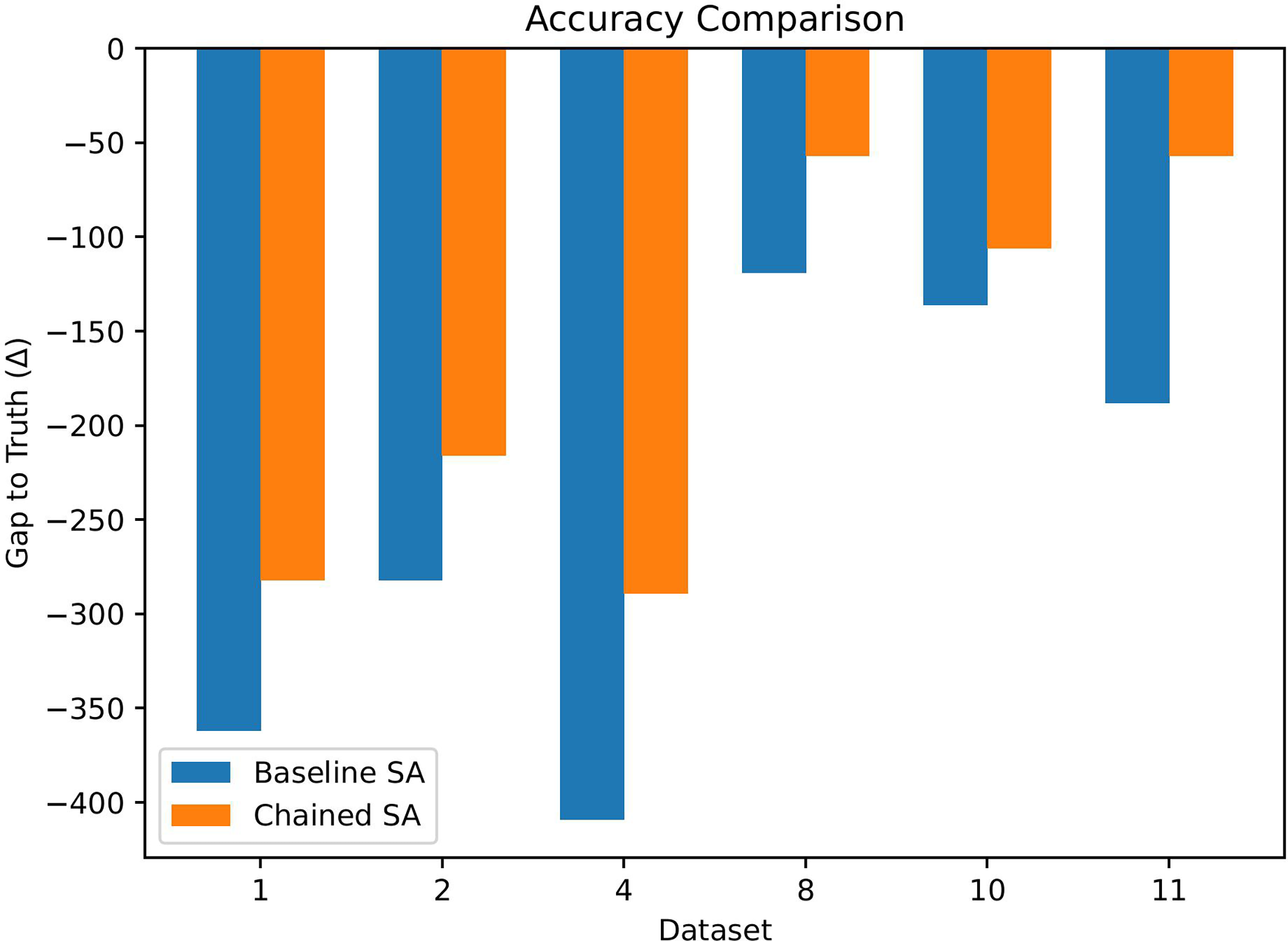
Figure 1 provides a visual comparison of the baseline and chaining-aware SA variants, showing that chaining generally moves the solution closer to Truth across most datasets.

FIG. 1.

Comparison of baseline and chaining-aware simulated annealing in terms of gap to the upper bound Truth on representative datasets. Values closer to 0 indicate better agreement with the dataset-specific reference upper bound. Chaining generally reduces the gap relative to the baseline across most datasets.

5.4.5. Efficiency

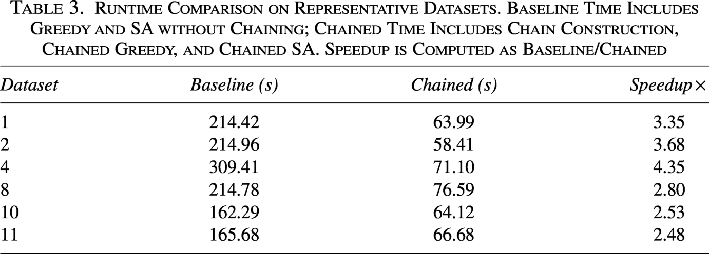
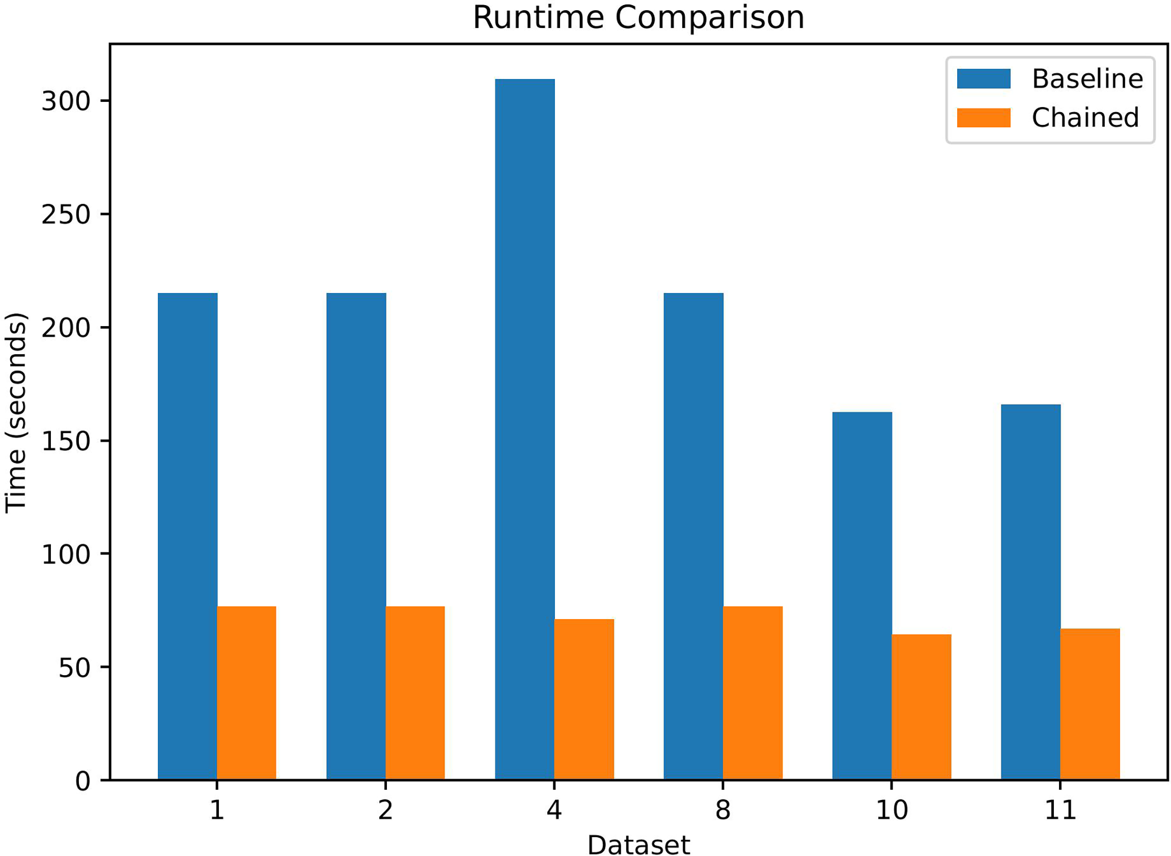
Table 3 shows consistent runtime gains with chaining across the representative datasets. On average, the total wall–clock time decreases from $\approx 213.6$ s (baseline) to $\approx 66.8$ s (chained), corresponding to a mean speedup of $\approx 3.20 \times$ (median $\approx 3.02 \times$ ).

Table 3.
Runtime Comparison on Representative Datasets. Baseline Time Includes Greedy and SA without Chaining; Chained Time Includes Chain Construction, Chained Greedy, and Chained SA. Speedup is Computed as Baseline/Chained

Dataset Baseline (s) Chained (s) Speedup $\times$

1 214.42 63.99 3.35

2 214.96 58.41 3.68

4 309.41 71.10 4.35

8 214.78 76.59 2.80

10 162.29 64.12 2.53

11 165.68 66.68 2.48

Dataset	Baseline (s)	Chained (s)	Speedup $\times$
1	214.42	63.99	3.35
2	214.96	58.41	3.68
4	309.41	71.10	4.35
8	214.78	76.59	2.80
10	162.29	64.12	2.53
11	165.68	66.68	2.48

Although Table 3 reports end-to-end runtimes, the dominant savings arise in the SA phase: restricting the search to block-consistent regions substantially reduces the number of candidate evaluations per iteration. The overhead of chain construction is negligible, and the Greedy stage also benefits from operating within precomputed blocks.

As shown in Figure 2, chaining yields substantial runtime reductions across all representative datasets.

FIG. 2.

Runtime comparison between baseline and chaining-aware methods on representative datasets. Reported times correspond to end-to-end execution. Chaining substantially reduces total runtime across all shown datasets.

5.4.6. Scalability

Collinear chaining reduces the effective search space by focusing computation within an ordered set of conserved blocks and their margins. This pruning makes both greedy selection and stochastic refinement more efficient at longer sequence lengths: the chaining step scales near-linearly in the number of anchors, while refinement depends on the number of block positions rather than the full sequence length.

Combined with the observed $\approx 3.20 \times$ runtime speedup and consistent or improved accuracy, these results suggest favorable scalability as scaffold length and gap count increase.

6. CONCLUSION

In this article, we study the multi-scaffold filling problem and report empirical results based on both theoretical and practical approaches. We formulate the problem using DP and develop practical heuristic methods, including greedy initialization and SA, together with a chaining-based strategy to restrict the search space and improve computational efficiency. The complete empirical results are included in the Appendix as Table A1 and Table A2.

Certainly, there are many different versions of the problem and further investigations are needed—for instance, what about implementing the DP method on a parallel computer? We are especially interested in practical algorithms. Which are likely to obtain useful empirical results. We conclude the article with the following summaries.

6.1. What makes the problem hard

A full, exact DP solution over all gap assignments is not practical: the number of combinations grows exponentially, and even a single evaluation requires three global alignments. We therefore use NW (BLOSUM62, linear gaps) as our final scoring oracle, while avoiding recomputing it at every local move during search. This motivates the use of heuristic strategies and chaining-based restrictions to efficiently explore the search space.

6.2. Our practical approach

We incorporate a collinear-chaining strategy on top of two standard heuristics (Greedy and SA). Chaining identifies short shared k-mer anchors between scaffolds, links them into ordered blocks, and restricts Greedy/SA to mutate gaps only within or near these blocks. During search, we update fast block-based scores, and all final results are recomputed using exact NW scoring for fair comparison. This approach significantly reduces the search space and improves computational efficiency while maintaining competitive alignment quality.

6.3. What we observed

Across our datasets, the chaining-aware variants achieve comparable or improved accuracy in most cases while reducing total runtime by about 3– $4 \times$ on average. Most of the speedup appears in the SA phase because the restricted neighborhood is smaller and more coherent. Greedy often lands close to the reference-based upper bound, while SA can further improve some cases, though not consistently under the NW metric.

6.4. Limitations

(1) We evaluate against a single reference per dataset; biological truth may not always coincide with the NW optimum. (2) We fix BLOSUM62 and a linear gap penalty; different scoring schemes (e.g., affine gaps or structure-aware scores) could change outcomes. (3) Our anchors are exact short k-mers; spaced seeds or profile-based anchors may perform better in indel-rich regions. (4) Gap candidate sets are assumed small and plausible; overall solution quality depends on how these sets are constructed. (5) Experiments are conducted on curated datasets under a single hardware/software setup; performance may vary under different conditions.

6.5. Future directions

Promising extensions include: faster and parallel implementations of NW (SIMD/GPU) or banded/sparse variants; richer seeding strategies and adaptive block construction; alternative objectives that combine NW with structural or biochemical priors (and possibly multiple references); more robust local search methods (e.g., tabu search, iterated local search, or small beam search); and scaling to more than three scaffolds with consensus-aware chaining.

6.6. Takeaway

Combining exact NW for final evaluation with a lightweight chaining layer for search makes multi-scaffold gap filling both practical and efficient, while maintaining competitive alignment accuracy.

AUTHORS’ CONTRIBUTIONS

I.M.: Investigation, methodology, software, writing—reviewing and editing. X.L. Conceptualization, methodology, writing—reviewing. L.Q.: Conceptualization, methodology, writing—reviewing. L.W.: Conceptualization, methodology, writing—reviewing. B.Z.: Conceptualization, investigation, methodology, writing—reviewing and editing.

Footnotes

ACKNOWLEDGMENT

The authors thank anonymous reviewers for helpful comments.

AUTHOR DISCLOSURE STATEMENT

No competing financial interests exist.

FUNDING INFORMATION

This research is supported by NSF under awards 2307571, 2307572, 2307573, and 2434487. L.W. is supported by a grant from NNSF of China (project 61972329) and GRF grants from Hong Kong SAR, China (CityU 11218423 and CityU 11218821).

Appendix

References

Aebersold

, Mann

. Mass spectrometry-based proteomics. Nature 2003;422(6928):198–207.

Badal

, Qingge

, Liu

, et al. Novel probabilistic and machine learning approaches for the protein scaffold gap filling problem. J Comput Sci Technol 2025;40(4):1109–1123.

Badal

, Qingge

, Liu

, et al. Probabilistic and machine learning models for the protein scaffold gap filling problem. In: Bioinformatics Research and Applications—20th International Symposium, ISBRA 2024, Kunming, China, July 19–21, 2024, Proceedings, Part III, volume 14956 of Lecture Notes in Computer Science . ( Peng

, Cai

, Skums

, eds). Springer; 2024, pp. 28–39.

Calabro

, Impagliazzo

, Paturi

. The complexity of satisfiability of small depth circuits. In: Parameterized and Exact Computation, 4th International Workshop, IWPEC 2009, Copenhagen, Denmark, September 10–11, 2009, Revised Selected Papers, volume 5917 of Lecture Notes in Computer Science . ( Chen

and Fomin

, eds). Springer; 2009, pp. 75–85.

DiMaggio

Jr , Young

, Baliban

, et al. A mixed integer linear optimization framework for the identification and quantification of targeted post-translational modifications of highly modified proteins using multiplexed electron transfer dissociation tandem mass spectrometry. Mol Cell Proteomics 2009;8(11):2527–2543.

Edman

. A method for the determination of the amino acid sequence in peptides. Arch. Biochem 1949;22:475–476.

Feng

, Fernau

, Zhu

. Optimal bridge, twin bridges and beyond: Inserting edges into a road network to minimize the constrained diameters. In: Algorithmic Aspects in Information and Management – AAIM 2024 – 18th Annual International Conference, Dallas, Texas, September 21–23, 2024. Proceedings, volume 15179 of Lecture Notes in Computer Science . ( Ghosh

and Zhang

, eds). Springer; 2024, pp. 94–108.

Henikoff

, Henikoff

. Amino acid substitution matrices from protein blocks. Proc Natl Acad Sci U S A 1992;89(22):10915–10919.

Impagliazzo

, Paturi

. On the complexity of k-sat. J. Comput. Syst. Sci 2001;62(2):367–375.

10.

Liu

, Dekker

LJM

, Wu

, et al. De novo protein sequencing by combining top-down and bottom-up tandem mass spectra. J Proteome Res 2014;13(7):3241–3248.

11.

Needleman

, Wunsch

. A general method applicable to the search for similarities in the amino acid sequence of two proteins. J Mol Biol 1970;48(3):443–453.

12.

Qingge

, Badal

, Annan

, et al. Generative AI models for the protein scaffold filling problem. J Comput Biol 2025;32(2):127–142.

13.

Qingge

, Liu

, Zhong

, et al. Filling a protein scaffold with a reference. IEEE Trans Nanobioscience 2017;16(2):123–130.

14.

Rizzo

, Cáceres

, Mäkinen

. Practical colinear chaining on sequences revisited. In: Bioinformatics Research and Applications - 21st International Symposium, ISBRA 2025, Helsinki, Finland, August 3–5, 2025, Proceedings, Part II, volume 15757 of Lecture Notes in Computer Science . ( Tang

, Lai

, Cai

, Peng

, Wei

, eds). Springer; 2025, pp. 203–216.

15.

Schaefer

. The complexity of satisfiability problems. In: Proceedings of the 10th Annual ACM Symposium on Theory of Computing, STOC . ( Lipton

, Burkhard

, Savitch

, Friedman

, Aho

, eds). ACM; 1978, pp. 216–226.

16.

Sturtz

, Zhu

, Liu

, et al. Deep learning approaches for the protein scaffold filling problem. In: 2022 IEEE 34th International Conference on Tools with Artificial Intelligence (ICTAI) . IEEE; 2022, pp. 1055–1061.

17.

Sturtz

, Annan

, Zhu

, et al. A convolutional denoising autoencoder for protein scaffold filling. In: Bioinformatics Research and Applications - 19th International Symposium, ISBRA 2023, Wrocław, Poland, October 9–12, 2023, Proceedings, Vol. 14248 of Lecture Notes in Computer Science . ( Guo

, Mangul

, Patterson

, Zelikovsky

, eds). Springer; 2023, pp. 518–529.

18.

Tran

, Rahman

, He

, et al. Complete de novo assembly of monoclonal antibody sequences. Sci Rep 2016;6(1):31730.

19.

Wang

, Pérez-Santiago

, Katz

, et al. Peptide identification from mixture tandem mass spectra. Mol Cell Proteomics 2010;9(7):1476–1485.

20.

Wang

, Bourne

, Bandeira

. Mixgf: Spectral probabilities for mixture spectra from more than one peptide. Mol Cell Proteomics 2014;13(12):3688–3697.

21.

Williams

. A new algorithm for optimal 2-constraint satisfaction and its implications. Theor Comput Sci 2005;348(2–3):357–365.

22.

Zhu

, Liu

. A graph-based approach for proteoform identification and quantification using top-down homogeneous multiplexed tandem mass spectra. BMC Bioinform 2018;19S(9):161–168.

Dataset	Baseline		Chained		Truth	$Δ$ SA
Dataset	Greedy	SA	Greedy	SA	Truth	Base	Chained
1	3032	2980	3045	3060	3342	−362	−282
2	3078	3060	3102	3126	3342	−282	−216
4	3038	2930	3049	3050	3339	−409	−289
8	2477	2542	2473	2604	2661	−119	−57
10	2032	2141	2034	2171	2277	−136	−106
11	2039	2086	2039	2217	2274	−188	−57

Investigations on Multiple Protein Scaffold Filling

Abstract

Keywords

1. INTRODUCTION

2. PRELIMINARIES

2.1. Problems

3. A LOWER BOUND FOR THE k TOP-DOWN SCAFFOLD PROBLEM

4.1. Two or three scaffolds, no reference

4.2. Other solvable cases

5. PRACTICAL ALGORITHMS FOR FILLING THREE SCAFFOLDS

5.1. Problem setting and motivation

5.1.1. Notation

5.1.2. Scoring objectives

5.1.4. Computational difficulty

5.1.5. Algorithmic families

5.1.6. Assumptions and practical choices

5.1.7. Evaluation goals

5.2.1. NW (baseline alignment)

5.2.1.1. Setup

5.2.1.3. Use in our pipeline

5.2.1.4. Practical notes

5.2.2. Greedy heuristic

5.2.2.1. Idea

5.2.2.2. Pseudo-code

5.2.2.4. Strengths and limitations

5.2.3. Simulated annealing

5.2.3.1. Idea

5.2.3.2. Neighborhood

5.2.3.3. Pseudo-code

5.2.3.5. Complexity

5.2.3.6. Strengths and limitations

5.2.4. Collinear chaining

5.2.4.1. Idea

5.2.4.2. Pairwise anchors

5.2.4.3. Collinear chain DP

5.2.4.4. Blocks and consensus

5.2.4.5. Block‐sum proxy for fast scoring

5.2.4.6. Integration into greedy and SA

5.2.4.7. Complexity and speed

5.2.4.8. Practical notes

5.3. Experimental setup

5.3.1. Datasets

5.3.2. Fragments/candidate sets

5.3.3. Hardware and software

5.3.4. Initialization and randomness

5.3.5. Hyperparameters

Table 1. Simulated Annealing Schedules Used in the Experiments Variant Initial temp T 0 Cooling rate Max iterations Baseline SA 150 0.98 5000 Chained SA 6 0.999 8000

5.3.7. Outputs recorded

5.4. Results

5.4.1. Dataset structure

5.4.2. Scoring

5.4.3. Table overview

5.4.4. Accuracy

6. CONCLUSION

6.1. What makes the problem hard

6.2. Our practical approach

6.3. What we observed

6.4. Limitations

6.5. Future directions

6.6. Takeaway

AUTHORS’ CONTRIBUTIONS

Footnotes

ACKNOWLEDGMENT

AUTHOR DISCLOSURE STATEMENT

FUNDING INFORMATION

Appendix

References

Table 1.
Simulated Annealing Schedules Used in the Experiments

Variant Initial temp $T_{0}$ Cooling rate Max iterations

Baseline SA 150 0.98 5000

Chained SA 6 0.999 8000