Incorporating Spatial Autocorrelation into Optimal Mobility Control Models in Epidemics: A Case Study using Moran’s I Statistic

Abstract

Human mobility plays a key role in many epidemics, as evident during the COVID-19 pandemic. As a control measure, mobility restrictions are implemented in and between spatial units, such as states, districts, and local municipalities. The spatial autocorrelation of incidence of disease allows health authorities to decide the mobility restrictions of a spatial unit by observing the incidence of neighboring units. Such a case is tested in this work using a Susceptible-Infected-Recovered (SIR) model for COVID-19 that emphasizes the use of Moran’s $I$ as a measure of spatial autocorrelation. The model is equipped with a parametric design that assimilates the spatial variation of incidence into mobility control. The clustering effect given by positive autocorrelation is observed as a risky case for transmission that calls for severe restrictions. The model is later adapted into an optimal control scenario that addresses the fact that a country should be open to usual economic activities while ensuring lower transmission. Numerical experiments show how Moran’s $I$ classifies transmission risk to achieve optimal mobility control. This approach of incorporating spatial autocorrelation can be used in similar contexts of other dynamical systems.

Keywords

compartmental model mobility control spatial autocorrelation

1. Introduction

In response to epidemics and pandemics, health authorities implement control measures to monitor human mobility. These controls are often enforced on spatial units declared by administrative boundaries, such as states, provinces, districts, and cities, considering the spatial distribution of infected cases and the subsequent risk posed by human density and mobility (Lee & Eom, 2024; Liu et al., 2020a). There are many diseases that are influenced by spatial factors, such as human mobility (eg. influenza), population density (eg. measles), the geographic distribution of weather patterns (eg. dengue), and region-specific health interventions (eg. malaria). Spatial analysis of epidemics paves the way for effective control measures (Pfeiffer et al., 2008). In controlling epidemics, it is essential to identify spatial units with varying levels of incidence, focusing on the incidence of their neighboring units as well (Abdulhafedh, 2017; Anselin, 2020). For example, a high-incidence cluster of units could rapidly transmit the disease to surrounding low-incidence units. Such identification help determine appropriate control measures (Liu et al., 2024). Research in this field has been trending, with improved access to surveillance data, despite some limitations (Franch-Pardo et al., 2020; Lan & Delmelle, 2023). The COVID-19 pandemic has established a good platform in this regard (Kjellesvig et al., 2025; Srinivasan et al., 2025).

In the context of spatial analysis, Moran’s $I$ statistic is a widely used spatial autocorrelation measure that indicates the degree to which similar observations occur in nearby spatial units (Jackson et al., 2010). While measures like Geary’s $C$ or Getis–Ord $G^{*}$ capture local patterns, Moran’s $I$ effectively summarizes overall spatial trends for guiding mobility control (Petronilla et al., 2017). The work presented here trials COVID-19 transmission to develop a framework for optimal mobility control. It is often a matter of controversy whether to lift lockdowns for day-to-day activities or continue restricting mobility for the betterment of public health (Fu et al., 2022). Analyzing such optimal control scenarios is important in exploring dynamics with targets and limitations in the field (Bolzoni et al., 2017; Khan et al., 2022; Lee & Castillo-Chavez, 2015). The applicability of Moran’s $I$ statistic in optimal control scenarios is rarely addressed in the literature, although spatial studies on epidemics are available (Lan & Delmelle, 2023). The importance of analyzing the spatiotemporal distribution of many diseases is evident, especially for countries with economic hardships (Sun et al., 2017). A preliminary optimal control analysis of COVID-19, considering only usual mobility rates, is available in (Hansana et al., 2024). It revealed optimal lockdown strategies that distinguish between designated regions and within regions. Both local and cross-region mobility restrictions were crucial for minimizing transmission from the outset of the COVID-19 pandemic (Oka et al., 2021). In another spatiotemporal study of COVID-19, spatial variations were investigated via Moran’s $I$ , and a risk map was produced using Moran scatter plots (Ganegoda et al., 2023). Decision support systems to mitigate disease transmission can be well equipped with techniques that involve spatial autocorrelation (Liu et al., 2020b; Massachusetts Institute of Technology, 2020).

The main objective of this work is to emphasize the incorporation of spatial autocorrelation into epidemic models with its utility in optimal control problems. The study was motivated by another investigation that includes a spatiotemporal analysis of COVID-19 (Ganegoda et al., 2022). In that study, numerical experiments were carried out on a measure that reflects specific risk levels of the disease. Alternatively, the current work targets the direct minimization of a cost functional that incorporates both infected cases and mobility controls, rather than testing a measure for given control inputs. This interchange enables investigating different spatial variations, which is a challenging task by the approach in (Ganegoda et al., 2022).

The current work was further motivated by the differences in the depth and breadth of mobility restrictions across various countries, highlighting the absence of a common practice, and hence, understanding proper intervention becomes challenging (Du et al., 2021; Oka et al., 2021). Meanwhile, already formulated optimal control epidemic models provide a good platform to introduce new spatially driven mobility controls (Adepoju & Olaniyi, 2021; Nepomuceno et al., 2021). Controls on vaccination, treatment, testing capacity, hygiene practices, vector-species control, etc., are frequently available in such models in addition to controls on close contact or mobility (Aldila et al., 2013; Disselhorst, 2021). Stability analysis stands as a pivotal aspect that primarily ensures conditions for a varying quantity to be stable in the long run (Martcheva, 2015; Michel et al., 2015). With regard to spatial variations, stability of equilibrium levels (disease-free and endemic) as well as unstable scenarios overwhelming control strategies are worth identifying (Boehmer et al., 2010; Chawla et al., 2024; Hale, 1969; Salman et al., 2023).

2. Spatial Context

A scenario development for mobility control is presented here with the insight of incorporating spatial autocorrelation.

2.1. Scenario Development and Data

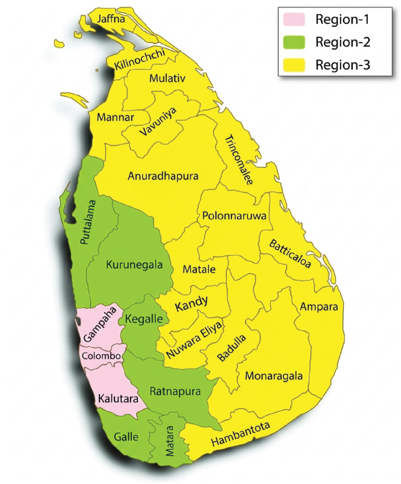
In this case study, the 25 administrative districts of Sri Lanka were classified into three main regions as Region-1: 3 districts (Colombo, Gampaha, and Kalutara); Region-2: 6 districts (Galle, Matara, Ratnapura, Kegalle, Kurunegala, and Puttalam); and Region-3: 16 districsts (all the other districts) (Figure 1). Region-1 has a high population density and is highly urbanized, with numerous commercial and administrative hubs (Central Bank of Sri Lanka, 2020; Department of Census and Statistics - Sri Lanka, 2022). Thus, Region-1 has high human mobility and it attracts humans from other districts as well. Hence, Region-1 mainly contributed to the diffusion of COVID-19 transmission to other areas. This diffusion is more responsible for the neighboring Region-2 and next for Region-3.

Figure 1.

Region map for the case study of Sri Lanka, illustrating the three regions and the allocation of districts within each region.

During the early stage of the COVID-19 outbreak, Region-1 reported a high number of cases, indicating that the virus spread from urban areas to rural ones. This urban-to-rural transmission pattern demonstrates how urban centers acted as initial hotspots, facilitating the wider spread of COVID-19 throughout the country (Amaratunga et al., 2020; Daily Mirror, 2021b; The World Bank, 2020). Separation of three regions was further influenced by the density of COVID-19 confirmed cases (positive for antigen test) reported during the observation period, from April 14 to May 15, 2021. Region-1 and Region-3 were accountable for the largest and smallest population densities, 1588.25 and 180.37 individuals/km $^{2}$ , respectively, with confirmed cases densities of 5.85 and 0.18, respectively. COVID-19 data were retrieved from the Epidemiology Unit of the Ministry of Health, Sri Lanka (Epidemiology Unit – Ministry of Health Sri Lanka, 2021), and the observation period was chosen so since it was the start of a major spread after the local new year festival season in 2021 (Sri Lanka Army, 2021; Sunday Times Editorial, 2021; The World Bank, 2021b). Required census data are available in the Department of Census and Statistics - Sri Lanka (Department of Census and Statistics - Sri Lanka, 2022).

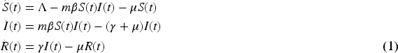
A Susceptible-Infected-Recovered (SIR) model was used, which has been a parsimonious approach, but mimics the main dynamics (Mohajan, 2022; Nur et al., 2018). The model (1) was introduced, incorporating the influence of human mobility that is subsequently driven by spatial variations in regional populations. $S (t)$ , $I (t)$ , and $R (t)$ represent the proportions of susceptible, infected, and recovered cases, respectively, with the assumption that the total population is constant (i.e., $S + I + R = 1$ ). Here, the proportion of infected individuals on a particular day is obtained by subtracting the total proportions of recovered and death cases from the total proportion of confirmed cases reported up to that day. In data processing, proportions were preferred over incidence to maintain the same scale $[0, 1]$ for infected compartments and control variables introduced later. This compatibility allows a convenient approach to selecting the corresponding weights in the optimal control analysis for the cost functional.

The parameter $Λ \in R^{+}$ (recruitment rate) and $μ \in R^{+}$ (removal rate) are treated as data-driven parameters, introduced to represent the net inflow and outflow of the $S I R$ proportions. Here, the inflow consists of natural births and immigration, and in addition, $Λ$ is supposed to account for the high vulnerability of COVID-19, which is typically not addressed by the transmission rate $β \in R^{+}$ . The parameter $β$ basically represents the transmissibility of the COVID-19 variant. Meanwhile, the outflow consists of natural deaths, emigration, and all removals due to immunity and vaccination. It was assumed that $Λ = μ$ to maintain a constant total population. The rate $Λ$ tallies in dimensions with the rate $μ$ since the populations are taken in proportions for $S (t), I (t)$ and $R (t)$ . The parameters $γ, m \in R^{+}$ represent the recovery rate and mobility rate, respectively.

\begin{aligned} \dot{S} (t) & = Λ - m β S (t) I (t) - μ S (t) \\ \dot{I} (t) & = m β S (t) I (t) - (γ + μ) I (t) \\ \dot{R} (t) & = γ I (t) - μ R (t) \end{aligned}

(1)

Here, the mobility rate $m$ was introduced as a dimensionless parameter coupled with the transmission rate $β$ to drive higher mobility towards higher transmission. Even though $m = 0$ results in no transmission, it is hardly feasible in practice.

The computation of $m$ using the gravity model has been explained elsewhere (Hansana et al., 2024). In brief, it takes the form $P_{1} P_{2} / r^{2}$ , where $P_{1}$ and $P_{2}$ are the populations of the two concerned regions and $r$ is the distance between those regions (Hong et al., 2019). In the preliminary parameter estimation (Subsection 2.4), Region-1 and Region-2 were taken for computation $m$ , assuming high mobility for the whole country during the said festival period. Higher population and case densities of these regions also supported this claim. Further manipulations of $m$ for optimal control scenarios in the long run will be explained in Subsection 4.1.

2.2. Spatial Autocorrelation

Spatial autocorrelation quantifies the correlation of an observation of interest (response variable) with itself across different spatial units, whereas temporal autocorrelation does so over time (Anselin, 2020; Lee, 2017; Moran, 1948). Moran’s $I$ , Geary’s $C$ , and Getis-Ord $G_{i}^{*}$ are the main spatial autocorrelation measures (Chen, 2013; Getis & Ord, 1995). Geary’s $C$ and Getis-Ord $G_{i}^{*}$ mostly articulate the local association of observations. However, Moran’s $I$ incorporates the deviation from the mean in assessing the association (Getis & Ord, 1992; Zhou & Lin, 2008). Such a formulation opens the door to better correlation when the spatial units are categorized into several regions, which is also the case in this study. In this work, global Moran’s $I$ formula shown in 2 was used to measure spatial autocorrelation (Chen, 2021).

I_{M o r a n} = (\frac{N}{\sum_{i = 1}^{N} \sum_{j = 1}^{N} w_{i j}}) \frac{\sum_{i = 1}^{N} \sum_{j = 1}^{N} w_{i j} (x_{i} - \bar{x}) (x_{j} - \bar{x})}{\sum_{i = 1}^{N} (x_{i} - \bar{x})^{2}}

(2)

Here,

x_{i}

and

x_{j}

are the observations of interest relevant to spatial units indexed by

i

and

j

. In this study, the infected proportion stands as the observation.

\bar{x}

is the mean of the observations of all

N

number of spatial units,

w_{i j}

is the spatial weight between spatial units

i

and

j

. The set of weights

w_{i j}

introduces spatial connectivity into Moran’s

I

formula, where different types of weights can be used, such as adjacency-based weights or distance-based weights (Smith, 2017). It is often expected to set

w_{i j}

with a high value when the spatial units

i

and

j

are close and vice versa. In this study, an adjacency-based case was employed, where

w_{i j} = 1

when two spatial units,

i

and

j

, are adjacent (i.e., they share a common boundary) and

w_{i j} = 0

otherwise. This choice was motivated by the view that people usually feel the risk of COVID-19 once the neighboring areas are affected.

Moran’s $I$ usually remains between $- 1$ and $1$ , where positive values tend to indicate that spatial units having high observations are closely located (High surrounded by High, H-H), whereas spatial units having low observations follow the same (Low surrounded by Low, L-L). Thus, positive autocorrelation reflects a clustering effect, indicating that neighboring units tend to have similar observations. Conversely, Moran’s $I$ tends to be negative for other options, such as Low surrounded by High (L-H) and High surrounded by Low (H-L). Such a negative autocorrelation indicates a dispersion effect that contrasts with the earlier clustering effect. When spatial units having High and Low are randomly distributed, Moran’s $I$ tends to zero (Schmal et al., 2017; Yamada, 2024). The next section describes how these clustering and dispersion effects articulate disease transmission.

2.3. Rationale of Spatial Variations - Clustering and Dispersion

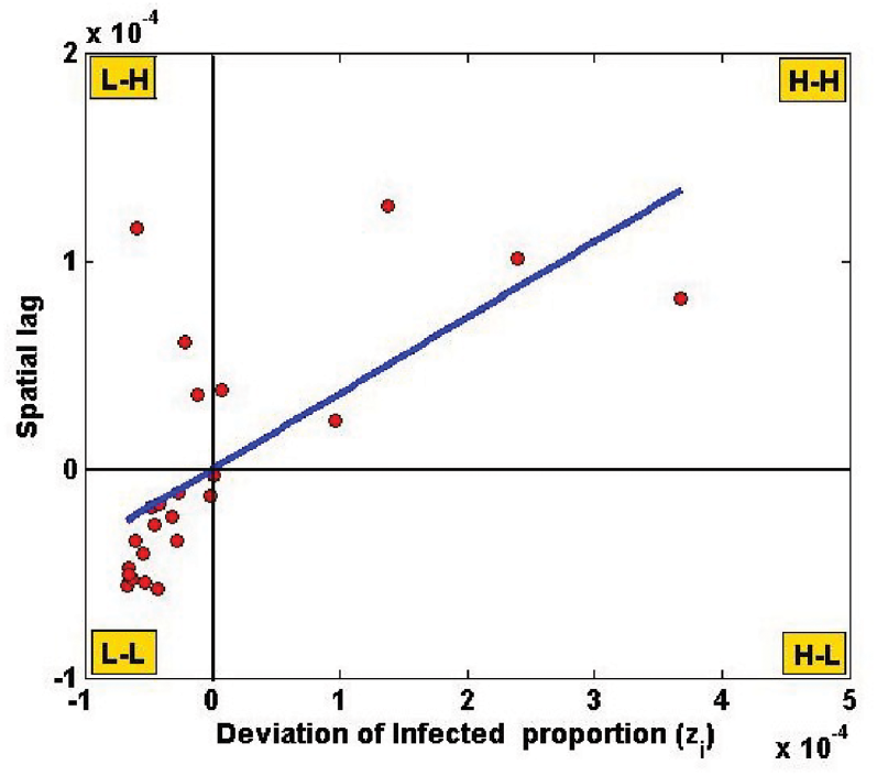
Since the infected proportion is time-variant, Moran’s $I$ is also time-variant when measured at each time point. However, it was manipulated to indicate the potential of transmission with spatial variations (clustering and dispersion). For this, the observation $x_{i}$ in formula (2) was taken as the total infected proportion of a spatial unit (a district, referred to by $i$ ) during the observation period (April 14 - May 15, 2021). Thus, it is assumed that Moran’s $I$ feature is a time-invariant parameter for further simulations. Figure 2 is the Moran scatter plot of infected proportion data during the observation period, taking 25 districts of Sri Lanka as spatial units. Here, the x-axis represents deviations $z_{i} = x_{i} - \bar{x}$ while the y-axis stands for the so-called spatial lag $\sum_{j = 1}^{n} w_{i j} z_{j}$ , positioning their means at the origin $(0, 0)$ . Then the slope of the linear regression line is the same as Moran’s $I$ (Anselin, 1996). A positive autocorrelation was found ( $I_{M o r a n} = 0.36$ ), indicating a clustering effect.

Figure 2.

Moran’s scatter plot of infected proportions across 25 districts of Sri Lanka, showing spatial autocorrelation.

Clustering increases the risk of COVID-19 transmission, whereas dispersion reduces it. This is mainly due to the fact that diffusion from high to low is well supported when spatial units with high proportions of infected are clustered together, particularly in highly dense and mobilized areas (Sigler et al., 2021; Yao et al., 2021). One of the COVID-19 studies in Indonesia found a higher spread in the second wave compared to the first wave, as indicated by a higher degree of clustering, measured by Moran’s $I$ (Rendana et al., 2021). In another study conducted in China, high-risk areas and their associated levels of risk with environmental factors were identified through positive autocorrelation, which exhibited a clustering effect (Han et al., 2021). Several studies have revealed a higher spread due to increased clustering over time periods or regions (Andrews et al., 2021; Ma et al., 2022). Upon further examination, our case study also explored region-wise spatial variations, which were coupled with controlling the transmission rate in the SIR model.

The spatial autocorrelation estimates, calculated from infected proportions across the 25 districts of Sri Lanka, may be influenced by spatial heterogeneity in reporting, testing rates, or population differences (Epidemiology Unit – Ministry of Health Sri Lanka, 2021). These factors can affect Moran’s $I$ values and, consequently, the recommended mobility controls, so the results should be interpreted with caution.

2.4. Moran-Induced Mobility Control

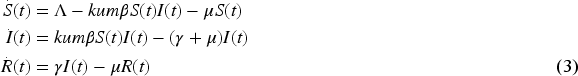
Mobility control was incorporated into the model (1) by introducing a weight for the transmission rate $β$ . This weight, $k u$ , named Moran-induced mobility control, consists of two routines, where $k$ represents spatial variations via Moran’s $I$ and $u \in [0, 1]$ indicates the level of mobility control. Here, the aim was to give an indirect influence on the transmission rate $β$ . by the spatial measure $k$ that brings the clustering feature. Even for the same $β$ , higher $k$ (higher clustering) leads to a higher infected proportion according to our model structure. Indeed, this is a causal mechanism; it can be justified as mobility control between high-risk neighboring areas reduces the proportion of subsequent infections.

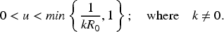
The modified model is available in (3). To infuse Moran’s $I$ as a positive parameter, the scaled version $k = \frac{I_{M o r a n} + 1}{2} \in [0, 1]$ was introduced with fixed bounds $- 1$ and $1$ for Moran’s $I$ (Böck et al., 2017). By this new scaling, $k \to 1$ (i.e., $I_{M o r a n} \to 1$ ) refers more to positive autocorrelation, while $k \to 0$ (i.e., $I_{M o r a n} \to - 1$ ) suggests negative autocorrelation. For a given $k$ , one can refer to $u$ as self-control of mobility. Self-control is defined by voluntary individual behaviors such as social distancing and travel limitations, which are typically observed during the emergence of a new wave of infections. However, since compliance with these measures is often inconsistent, stricter mobility restrictions are imposed by the government. Consequently, the term self-control is applied when no optimal control plan is implemented, as described in Section 4.

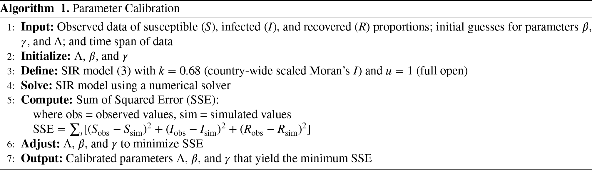
Subsequently, $u \to 0$ implies more mobility control, probably by government intervention and $u \to 1$ stands for relaxing the control. Terms $k$ and $u$ behave in opposite ways in nature, as the risky clustering effect (increasing $k$ ) should reflect more control (decreasing $u$ ). It was set $u = 1$ in the calibration of $β$ , assuming the country is fully open in the said observation period (Algorithm 1).

\begin{aligned} \dot{S} (t) & = Λ - k u m β S (t) I (t) - μ S (t) \\ \dot{I} (t) & = k u m β S (t) I (t) - (γ + μ) I (t) \\ \dot{R} (t) & = γ I (t) - μ R (t) \end{aligned}

(3)

2.5. Calibration of Parameters

Daily COVID-19 data of $S$ , $I$ , and $R$ of the observation period were used to calibrate the unobservable parameters $Λ$ , $β$ , and $γ$ . Although these parameters are theoretically sound, measuring them in practice is a challenging task. Therefore, one should choose the values that best describe the data. This is performed through an error minimization process, where the gap between parametrized simulations and data is minimized (Stavroulakis et al., 2003). Algorithm 1 describes the minimization in a least-squares sense. In our case study, $I_{M o r a n} = 0.36$ for the whole country, which gives $k = 0.68$ . Moreover, $Λ = μ$ was set as an assumption for this case study (see subsection 2.1). The calibrated parameter values of model (3) are $β = 0.33$ , $Λ = 0.0011$ , $μ = 0.0011$ , and $γ = 0.069$ , respectively, where all parameters are measured in $(days)^{- 1}$ .

3. Stability Analysis

The objective of this section is to analyze long-term behavior of the model (3) for a prevailing self-control $u$ . A local stability analysis of equilibrium points was performed to identify a range for $u$ subject to various spatial variations (clustering, random and dispersion) by varying the scaled Moran’s $I$ ( $k$ ). Both disease-free and endemic equilibrium were tested for their stability (Fudolig & Howard, 2020).

3.1. Basic Reproduction Number and Testing Equilibria

The basic reproduction numbers $R_{0}$ and $R_{k}$ of the models (1) and (3) respectively are given in (4), which can be obtained by quantifying the secondary cases over infectious period (Cheneke, 2023; Martcheva, 2015). As per the parameter values in subsection 2.5, $R_{0} \approx 3$ .

\begin{aligned} R_{0} = \frac{m β Λ}{(γ + μ) μ} and R_{k} = \frac{k u m β Λ}{(γ + μ) μ} = k u R_{0} \end{aligned}

(4)

The relationship $R_{k} \leq R_{0}$ can be established as a result of Moran-induced mobility control $k u \leq 1$ . This guarantees lesser secondary infections when the control is applied. It is evident that $R_{k}$ increases as clustering effect increases ( $k \to 1$ ) or mobility control is relaxed ( $u \to 1$ ).

Disease-free and endemic equilibrium points of the model 3 are $(S_{d f}^{*}, I_{d f}^{*}, R_{d f}^{*}) = [\frac{Λ}{μ}, 0, 0]$ and $(S_{e}^{*}, I_{e}^{*}, R_{e}^{*}) = [\frac{Λ}{μ R_{k}}, \frac{Λ}{γ + μ} (1 - \frac{1}{R_{k}}), \frac{Λ γ}{μ (γ + μ)} (1 - \frac{1}{R_{k}})]$ respectively. First, a bifurcation analysis was carried out to check the existence of equilibrium infected proportion for a particular $R_{k}$ . It was assumed that $k \neq 0$ and $u \neq 0$ for realistic scenarios. It means that the extremes of full dispersion and full lockdown are neglected which do not influence the generality of $k u$ . Next, equlibria were tested for their stability with regard to self-control $u$ .

The following Theorem 1 shows that significant self-control is required to ensure the disease-free status amidst higher clustering effects. This is observed as the upper bound of $u$ is less for higher $k$ values.

Theorem 1

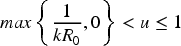
The necessary and sufficient condition for the self-control $u$ to exist and to achieve an asymptotically stable disease-free equilibrium is

0 < u < m i n {\frac{1}{k R_{0}}, 1}; where k \neq 0.

Proof.

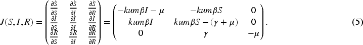
The Jacobian matrix of the model (3) can be obtained as follows

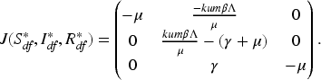
\begin{aligned} J (S, I, R) & = (\begin{matrix} \frac{\partial \dot{S}}{\partial S} & \frac{\partial \dot{S}}{\partial I} & \frac{\partial \dot{S}}{\partial R} \\ \frac{\partial \dot{I}}{\partial S} & \frac{\partial \dot{I}}{\partial I} & \frac{\partial \dot{I}}{\partial R} \\ \frac{\partial \dot{R}}{\partial S} & \frac{\partial \dot{R}}{\partial I} & \frac{\partial \dot{R}}{\partial R} \end{matrix}) = (\begin{matrix} - k u m β I - μ & - k u m β S & 0 \\ k u m β I & k u m β S - (γ + μ) & 0 \\ 0 & γ & - μ \end{matrix}) . \end{aligned}

(5)

The Jacobian at the disease-free equilibrium $(S_{d f}^{*}, I_{d f}^{*}, R_{d f}^{*}) = [\frac{Λ}{μ}, 0, 0]$ is

J (S_{d f}^{*}, I_{d f}^{*}, R_{d f}^{*}) = (\begin{matrix} - μ & \frac{- k u m β Λ}{μ} & 0 \\ 0 & \frac{k u m β Λ}{μ} - (γ + μ) & 0 \\ 0 & γ & - μ \end{matrix}) .

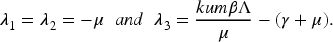
The eigenvalues of $J (S_{d f}^{*}, I_{d f}^{*}, R_{d f}^{*})$ are

λ_{1} = λ_{2} = - μ a n d λ_{3} = \frac{k u m β Λ}{μ} - (γ + μ) .

An equilibrium is asymptotically stable if and only if the eigenvalues have negative real part (Fudolig & Howard, 2020; Martcheva, 2015). The first two eigenvalues are negative since $μ > 0$ . The third eigenvalue is negative if and only if $\frac{k u m β Λ}{(γ + μ) μ} < 1$ and hence $u < \frac{(γ + μ) μ}{k m β Λ}$ .

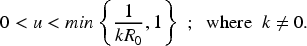
Note that $0 < u \leq 1$ and $0 < k \leq 1$ as per our defined and assumed ranges. Hence, the necessary and sufficient condition for the self-control $u$ to exist and to achieve asymptotically stable disease-free equilibrium is

0 < u < m i n {\frac{1}{k R_{0}}, 1}; where k \neq 0.

The following Theorem 2 is the counterpart of Theorem 1 for endemic equilibrium.

Theorem 2

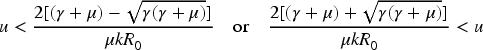
The necessary and sufficient condition for the self-control $u$ to exist and to achieve the stability of the endemic equilibrium is

m a x {\frac{1}{k R_{0}}, 0} < u \leq 1; where \frac{1}{k R_{0}} < 1 with k \neq 0.

Proof.

To ensure positive levels of the endemic equilibrium $(S_{e}^{*}, I_{e}^{*}, R_{e}^{*}) = [\frac{Λ}{μ R_{k}}, \frac{Λ}{γ + μ} (1 - \frac{1}{R_{k}}), \frac{Λ γ}{μ (γ + μ)} (1 - \frac{1}{R_{k}})]$ , it is required to have $R_{k} > 1$ . This establishes the condition

\frac{1}{k R_{0}} < u; where k \neq 0.

(6)

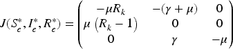
The Jacobian at the endemic equilibrium $(S_{e}^{*}, I_{e}^{*}, R_{e}^{*})$ is

J (S_{e}^{*}, I_{e}^{*}, R_{e}^{*}) = (\begin{matrix} - μ R_{k} & - (γ + μ) & 0 \\ μ (R_{k} - 1) & 0 & 0 \\ 0 & γ & - μ \end{matrix})

The eigenvalues of $J (S_{e}^{*}, I_{e}^{*}, R_{e}^{*})$ are

λ_{1} = - μ, λ_{2, 3} = \frac{- μ R_{k} \overset{+}{-} \sqrt{μ^{2} R_{k}^{2} - 4 μ (γ + μ) (R_{k} - 1)}}{2}

(7)

Here, the equilibrium is asymptotically stable if and only if the eigenvalues have negative real part (Fudolig & Howard, 2020; Martcheva, 2015). In this case, $λ_{1}$ is negative since $μ > 0$ . If the discriminant $Δ = μ^{2} R_{k}^{2} - 4 μ (γ + μ) (R_{k} - 1)$ in (7) is non-negative, then $λ_{2}$ and $λ_{3}$ are real and negative given that $R_{k} > 1$ . Otherwise for a negative discriminant, $λ_{2}$ and $λ_{3}$ are complex numbers having negative real part ( $- μ R_{k}$ ). Hence, a negative real part of all the eigenvalues are ensured.

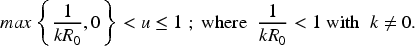
Again, claiming $0 < u \leq 1$ and $0 < k \leq 1$ as per our defined and assumed ranges and the earlier condition (6), the necessary and sufficient condition for the self-control $u$ to exist and to achieve asymptotically stable endemic equilibrium is

m a x {\frac{1}{k R_{0}}, 0} < u \leq 1

Theorem 2 shows that the lower bound on $u$ decreases as the clustering effect increases ( $k \to 1$ ,) making room for more mobility restrictions. Further to achieving endemic stability, the behavior of reaching infected proportion towards the endemic level can be classified as exponential decay and damped oscillations. Additional conditions for these cases can be derived as in Corollary 1 through the change of sign of the discriminant in (7).

Corollary 1

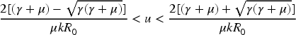
Additional conditions to achieve asymptotic stability with exponential decay of the endemic equilibrium can be established as:

u < \frac{2 [(γ + μ) - \sqrt{γ (γ + μ)}]}{μ k R_{0}} or \frac{2 [(γ + μ) + \sqrt{γ (γ + μ)}]}{μ k R_{0}} < u

and additional conditions to achieve asymptotic stability with damped oscillations of the endemic equilibrium can be established as

\frac{2 [(γ + μ) - \sqrt{γ (γ + μ)}]}{μ k R_{0}} < u < \frac{2 [(γ + μ) + \sqrt{γ (γ + μ)}]}{μ k R_{0}}

With the calibrated parameters in subsection 2.5, $\frac{1}{k R_{0}} = 0.4856$ . According to Theorem 1, the disease-free equilibrium is stable for $u \in (0, 0.4856)$ . This threshold of $0.4856 \approx 0.5$ indicates a mobility restriction stricter than halfway between full lockdown ( $u = 0$ ) and full open ( $u = 1$ ). In practice, the government can intervene with a plan of restricting mobility into a level less than $50 %$ of usual mobility. Theorem 2 implies that the endemic equilibrium is stable when $u \in (0.4856, 1]$ . Thus, the government should face the repercussions for managing infected population if the restrictions are not that strict. According to Corollary 1, $u \in (0.4856, 0.4875)$ should be the range for exponential decay, which is highly sensitive. Thus, damped oscillation would be the most probable appearance in endemic case. Health officials and policy makers should patiently handle such ups and downs. Although the bound $\frac{2 [(γ + μ) + \sqrt{γ (γ + μ)}]}{μ k R_{0}}$ applies on $u$ in Corollary 1, this is often redundant due to the restriction $u \leq 1$ . In fact, it is $123.83$ for the case produced above.

3.2. Sensitivity Analysis for Mobility Control

The facts in Theorem 1, Theorem 2 and Corollary 1 were further verified here. Sensitivity analysis of infected proportion was carried out by varying $u$ with three $k$ values (0.25, 0.5, and 0.75), which represent the dispersion, random, and clustering, respectively. These results are illustrated in Figure 3 - 5. As expected, Figure 3 indicates disease-free equilibrium for all $u$ values in a case of dispersion ( $k = 0.25$ ).Theorem 1 ensures $0 < u < m i n {1.32, 1} = 1$ for this case. In such a scenario, there is no risk of endemic equilibrium for any mobility level.

Figure 3.

Illustration of equilibrium points of the model (3) with $k = 0.25$ . The figure shows the disease-free condition (Theorem 1) where $0 < u \leq 1$ , indicating the range of self-control levels that maintain stability.

Figure 4.

Illustration of equilibrium points of the model (3) with $k = 0.5$ . The figure shows the disease-free condition (Theorem 1) for $0 < u < 0.66$ and the endemic condition (Theorem 2) for $0.66 \leq u \leq 1$ , indicating the ranges of self-control levels corresponding to each equilibrium.

Figure 5.

Illustration of equilibrium points of the model (3) with $k = 0.75$ . The figure shows the disease-free condition (Theorem 1) for $0 < u < 0.44$ and the endemic condition (Theorem 2) for $0.44 \leq u \leq 1$ , indicating the ranges of self-control levels corresponding to each equilibrium.

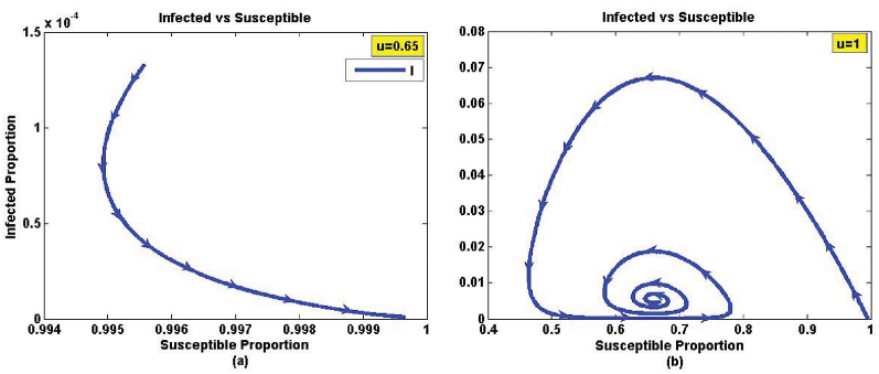
Figure 4 illustrates the equilibrium levels for $k = 0.5$ which represents random effect. The threshold value of $u$ to change from disease-free to endemic is $0.66$ . If the self-control is strict ( $u \to 0$ ) then the disease-free equilibrium is stable even under random effect. Moreover, the endemic equilibrium with damped oscillation occurs as the self-control is relaxed ( $u \to 1$ ) as a verification for Corollary 1.

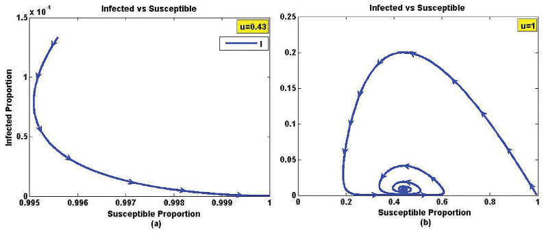
Figure 5 guides into a much smaller threshold for $u$ (0.44), resulting in $k = 0.75$ , which gives a case of clustering. Here, the self-control should be more strict to achieve a disease-free equilibrium. The endemic cases in Figure 5 show oscillations with higher amplitude, demonstrating significantly varying infected proportions before settling into equilibrium levels.

In summary, the existence of different bounds on self-control suggests to inspect region-wise spatial autocorrelation. Such analysis would designate more specific controls importantly in an optimal scenario. In the sequel, Section 4 assimilates this idea monitoring within a specific time frame rather than waiting for reaching equilibrium levels.

3.3. Bifurcation Analysis

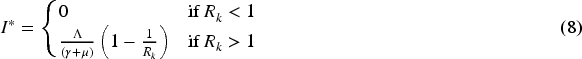
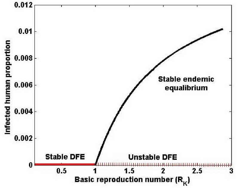
The following formulation (8) can be established for the equilibrium level of infected proportion $I^{*}$ . Here, $I_{e}^{*} = \frac{Λ}{(γ + μ)} (1 - \frac{1}{R_{k}})$ is an increasing function of $R_{k}$ that hints to a forward bifurcation. The relevant bifurcation diagram in Figure 6 confirms that the endemic equilibrium bifurcates in forward sense.

\begin{aligned} I^{*} = {\begin{cases} 0 & if R_{k} < 1 \\ \frac{Λ}{(γ + μ)} (1 - \frac{1}{R_{k}}) & if R_{k} > 1 \end{cases} \end{aligned}

(8)

Figure 6.

Bifurcation diagram showing both the disease-free equilibrium (DFE) and the endemic equilibrium of the model.

$I_{e}^{*}$ reaches a horizontal asymptote at $\frac{Λ}{(γ + μ)}$ as $R_{k}$ increases since $lim_{R_{k} \to \infty} [\frac{d I_{e}^{*}}{d R_{k}}] \to 0$ . Since $R_{k}$ is proportional to $k$ , it is clear that the forward bifurcation is driven by clustering effect. This facilitates a well-defined policy on mobility restriction, unlike in a backward bifurcation. Catastrophic scenarios might occur in backward cases as lowering reproduction number would push the disease to progress towards multiple stable states leaving disease-free equilibrium unstable (Dushoff et al., 1998; Guckenheimer & Holmes, 2013). However, the forward bifurcation suggests a progressive risk as reproduction number increases beyond $1$ .

4. Optimal Control

Maintaining a strict level of self-control for mobility can be challenging due to the heterogeneity of individual self-discipline. In this context, government intervention is essential, provided it is implemented within a suitable time frame. This section will provide an overview of how optimal mobility control strategies should be determined in the context of spatial variations. Primarily, the optimal objective should focus on the trade-off between the health costs incurred by the infected population and the economic losses due to mobility restrictions.

4.1. Extended Model for Mobility Control

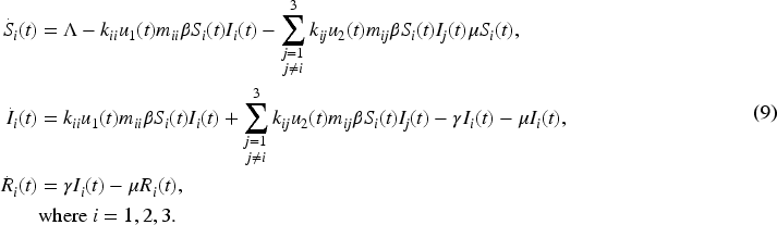
An optimal control problem was considered with three regions by categorizing 25 districts of Sri Lanka as given in the subsection 2.1. The extended model (9) carries region-wise compartments: $S_{i} (t)$ , $I_{i} (t)$ and $R_{i} (t)$ of Region- $i$ ; $i = 1, 2, 3$ representing respective proportions out of the population of the whole country. In what follows, the Moran-induced mobility control described in subsection 2.4 was also incorporated into the extended model. In the previous basic model (3), $u$ represented self-control of mobility, which was replaced by varying mobility control in the extended model. The control was considered in two ways, as within-region and between-regions, denoted by $u_{1} (t)$ and $u_{2} (t)$ , respectively. Mobility control is typically influenced by government interventions, and our aim was to investigate it in the context of a given optimal task.

\begin{aligned} \begin{aligned} {\dot{S}}_{i} (t) & = Λ - k_{i i} u_{1} (t) m_{i i} β S_{i} (t) I_{i} (t) - \sum_{\begin{matrix} j = 1 \\ j \neq i \end{matrix}}^{3} k_{i j} u_{2} (t) m_{i j} β S_{i} (t) I_{j} (t) μ S_{i} (t), \\ {\dot{I}}_{i} (t) & = k_{i i} u_{1} (t) m_{i i} β S_{i} (t) I_{i} (t) + \sum_{\begin{matrix} j = 1 \\ j \neq i \end{matrix}}^{3} k_{i j} u_{2} (t) m_{i j} β S_{i} (t) I_{j} (t) - γ I_{i} (t) - μ I_{i} (t), \\ {\dot{R}}_{i} (t) & = γ I_{i} (t) - μ R_{i} (t), \\ where i = 1, 2, 3. \end{aligned} \end{aligned}

(9)

The risk from asymptomatic individuals is reflected in the infected compartments, as a higher proportion of infections suggests a greater number of asymptomatic carriers. There are no restrictions on the mobility of infected individuals. The term $S_{i} (t) I_{i} (t)$ represents interactions within a region, while $S_{i} (t) I_{j} (t)$ indicates interactions between regions.

The notion of the scaled Moran’s $I$ (parameter $k$ ) should also be extended to region-wise cases. The approach was to replace $k$ by $k_{i j}$ , which represents scaled Moran’s $I$ considering all spatial units (districts) in Region- $i$ and Region- $j$ . Spatial variations within a region, such as regional clustering, are therefore captured through the measures $k_{i i}$ , where these districts of Region- $i$ are considered as spatial units. Although it is acknowledged that disease transmission occurs at a micro-level within smaller localities, the present model is designed to incorporate broader macro-level dynamics through a simplified framework. Thus, there were three Moran-induced mobility controls for between-regions cases as $k_{12} u_{2} (t), k_{13} u_{2} (t)$ and $k_{23} u_{2} (t)$ . Here, $k_{13}$ is owed to take all spatial units (districts) in the country since mobility between Region-1 and Region-3 may be associated with Region-2 as well, according to the separation described in the subsection 2.1. The within-region cases should be designated as $k_{11} u_{1} (t), k_{22} u_{1} (t)$ and $k_{33} u_{1} (t)$ , where $k$ was replaced by $k_{i i}$ taking spatial units only in Region- $i$ ; $i = 1, 2, 3$ into account.

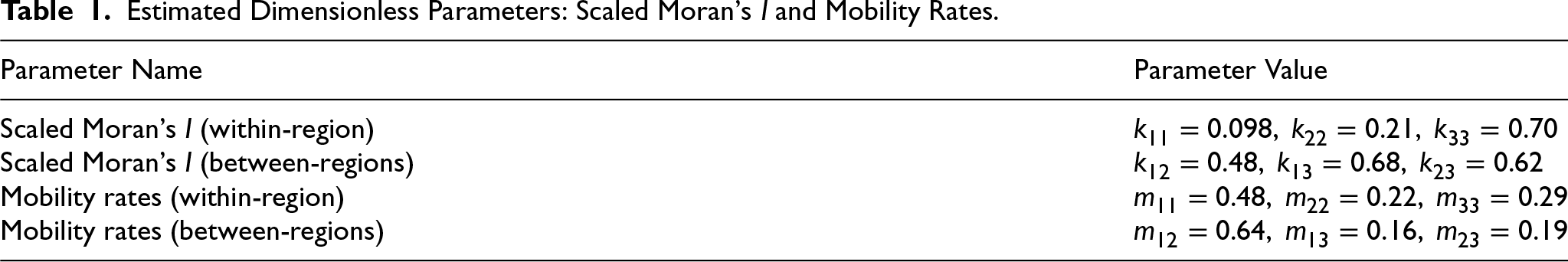
Usual mobility rates are also referred to as within-region ( $m_{i i}$ ) and between-region ( $m_{i j}$ ) cases, considered separately. It was assumed that $m_{i j} = m_{j i}$ . The gravity model is used to identify comparatively high or low mobility levels between spatial units, rather than focusing solely on attractiveness. For a given spatial unit, the mobility measure $m_{i j}$ is considered higher when it is associated with a region that has a larger population. These rates were estimated elsewhere as relative measures with census data (Hansana et al., 2024). As per that estimation, the within-region values ( $m_{11} = 0.48, m_{22} = 0.22, m_{33} = 0.29$ ) were based on population density and between-regions values ( $m_{12} = 0.64, m_{13} = 0.16, m_{23} = 0.19$ ) were associated with the gravity model. In the proposed modeling approach, the mobility rate was assumed to remain constant over time. The control variables were introduced as regulators of this baseline mobility. The parameter values of the extended model (9) are given in Table 1, in addition to those provided in the subsection 2.5.

Table 1.

Estimated Dimensionless Parameters: Scaled Moran’s $I$ and Mobility Rates.

Parameter Name	Parameter Value
Scaled Moran’s $I$ (within-region)	$k_{11} = 0.098, k_{22} = 0.21, k_{33} = 0.70$
Scaled Moran’s $I$ (between-regions)	$k_{12} = 0.48, k_{13} = 0.68, k_{23} = 0.62$
Mobility rates (within-region)	$m_{11} = 0.48, m_{22} = 0.22, m_{33} = 0.29$
Mobility rates (between-regions)	$m_{12} = 0.64, m_{13} = 0.16, m_{23} = 0.19$

4.2. Cost Functional and Solving Process

The optimal control problem was designed with the cost functional in (10) to compromise competing factors: infected proportions and mobility controls. The approach was to minimize the overall cost given by both factors over a specified time interval $[0, t_{f}]$ .

J (u_{1} (t), u_{2} (t)) = \int_{0}^{t_{f}} (\sum_{i = 1}^{3} W_{i} I_{i} (t) + \sum_{j = 1}^{2} V_{j} (1 - u_{j} (t))^{2}) d t

(10)

Here, the total cost of the infected proportions is given by the first summation with the weight constants $W_{1}, W_{2}$ , and $W_{3}$ . In our terminology, higher values of $u \in [0, 1]$ indicate lesser mobility restriction. Thus, higher $1 - u_{j} (t)$ ; $j = 1, 2$ indicates higher mobility restrictions that should be minimized to open the country for usual economic activities. The second summation in the cost-functional should be minimized for this, which contains within-region (by $1 - u_{1} (t)$ ) and between-regions (by $1 - u_{2} (t)$ ) cases, with weight constants $V_{1}$ and $V_{2}$ , respectively. In this study, a quadratic control term is used to represent the increasing cost of stricter interventions (as $u \to 0$ ). The squared form is conventionally applied to penalize higher control levels through a smooth and convex structure, facilitating the derivation of optimality conditions (Lenhart & Workman, 2007).

To solve the optimal control problem, the cost functional (10) should be minimized subject to the dynamics given by the extended model (9). An optimal pair $U^{*} (t) = (u_{1}^{*} (t), u_{2}^{*} (t))$ should be determined satisfying

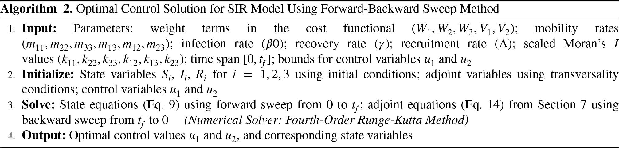
\begin{aligned} J (U^{*}) & = min {J (U) | U \in Ω}, \\ where Ω & = {(u_{1} (t), u_{2} (t)) \in (L^{1} [0, t_{f}])^{2}; 0 \leq u_{i} (t) \leq 1, t \in [0, t_{f}], i = 1, 2} . \end{aligned}

(11)

Corresponding state variables relevant to all compartments can also be determined. The necessary conditions of Pontryagin’s Maximum Principle are used to find the optimal solutions, and the standard results of optimal control theory provide a guarantee for the existence of optimal controls (Lenhart & Workman, 2007; Wendell Fleming, 1975). The required Hamiltonian process is shown in (7), and the Algorithm 2 shows the steps for numerical computations. The standard numerical method is the Forward-Backward Sweep Method, with the Fourth-Order Runge-Kutta Method serving as the ODE solver (Lenhart & Workman, 2007).

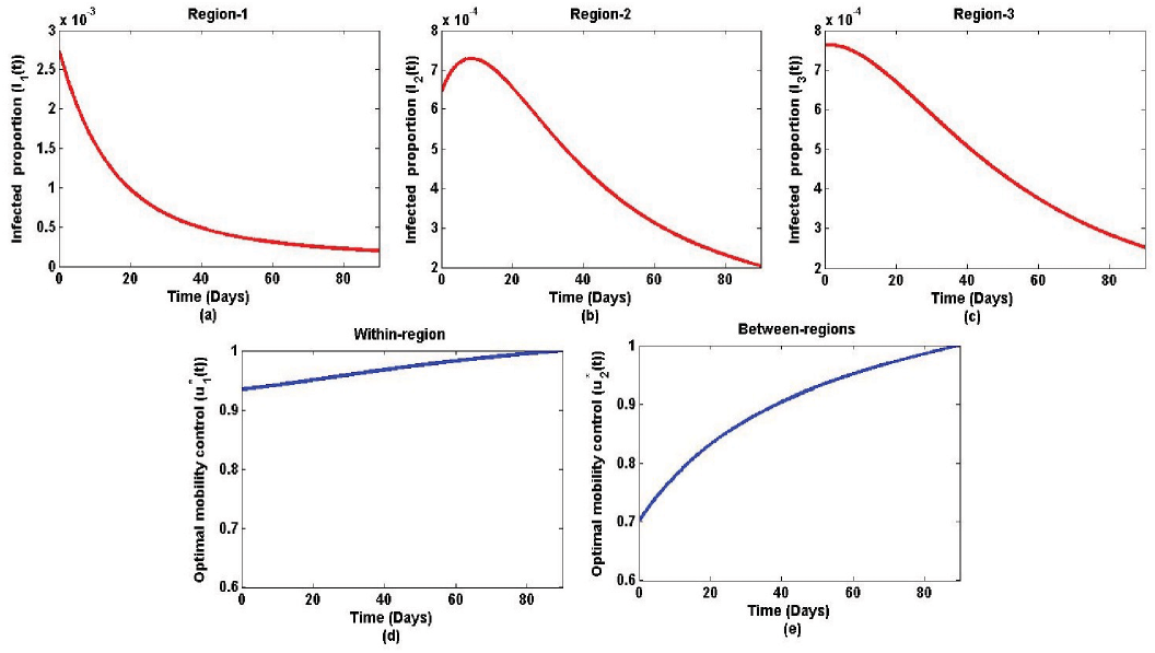
In our case study, an optimal solution obtained for a 3-month time frame is illustrated in Figure 7. This choice of three months was arbitrary, but based on an understanding of a medium-term control plan. It was assumed that the existing spatial variations of the regions, as estimated by the scaled Moran’s $I$ parameters, would continue to be the same. To balance the contributions of $I_{i}$ ’s and $(1 - u_{j})^{2}$ ’s in the cost $J (u_{1} (t), u_{2} (t))$ in a manner $W_{i} I_{i} = V_{j} (1 - u_{j})^{2}$ , the weights were selected as $W_{1} = W_{2} = W_{3} = 100$ and $V_{1} = V_{2} = 1$ . This choice is supported by an estimate based on the initial infected proportion of Region-1 ( $0.0025$ ) and the mid-value of $u_{j}$ ’s ( $0.5$ ), which gives $(1 - u_{j})^{2} = 0.25$ . Here, Region-1 was selected because it is the region that has the greatest vulnerability, as it is densely populated. Accordingly, the ratio was established as in (12).

\frac{W_{i}}{V_{j}} = \frac{(1 - u_{j})^{2}}{I_{i}} \approx \frac{0.25}{0.0025} \approx \frac{100}{1}

(12)

Region-wise dynamics of the infected proportions are depicted in Figure 7 (a)-(c), which shows a decline at the end as one should expect in curtailing disease transmission. It is worth noting that the mobility restrictions can be gradually relaxed as illustrated in Figure 7 (d)-(e), however, with more concern in between-regions. This was evident in Sri Lanka during the pandemic period as the government restricted crossing district or province borders, although no severe lockdown was imposed within-region (Daily Mirror, 2021a; Economynext, 2021). As per Figure 7 (e), mobility between-regions can be open

70 - 85 %

in the first month,

85 - 95 %

in the second month, and subsequently

95 - 100 %

in the last month.

Figure 7.

Variation of the infected proportions and corresponding optimal mobility controls. The parameters are provided in Table 1 and in the subsection 2.5. The weights of the cost functional are $W_{1} = W_{2} = W_{3} = 100$ and $V_{1} = V_{2} = 1$ .

4.3. Numerical Experiments of Optimal Mobility

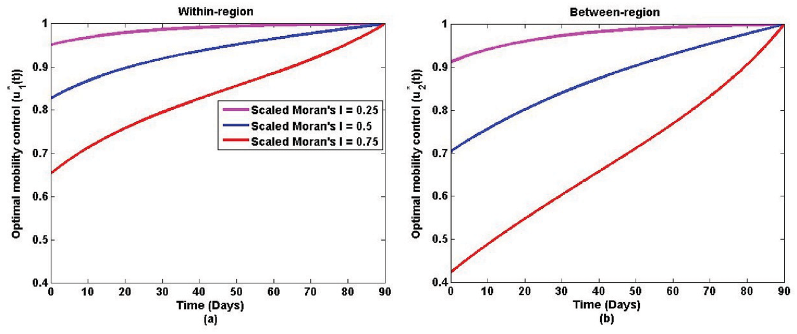
In this section, optimal mobility controls $u_{1}^{*} (t)$ and $u_{2}^{*} (t)$ are simulated by changing several parameters, particularly addressing spatial variations (clustering and dispersion) and cost functional contributions (via weights $W_{1}, W_{2}, W_{3}, V_{1}, V_{2}$ ). The simulations are conducted over a three-month time period, with the final time set as $t_{f} = 90$ days. Figure 8 shows the variations obtained subject to different scaled Moran’s $I$ parameters ( $k$ ). In this simulation, the same set of scaled Moran’s $I$ values was used for all regions, emphasizing the same spatial variation. Such a similarity might be developed as the disease progresses, as people across the country begin to experience similar levels of clustering or dispersion potential. For instance, hot spots may be detected only in one region during the observation period, but later become evident everywhere in the country. Accordingly to Figure 8, clustering effect (scaled Moran’s $I$ = 0.75) suggests more mobility restriction ( $u_{1} \approx 0.65$ and $u_{2} \approx 0.43$ ) at the early stage compared to dispersion effect (scaled Moran’s $I$ = 0.25) in both within-region ( $u_{1} \approx 0.97$ ) and between-regions ( $u_{2} \approx 0.91$ ). It categorically validates that clustering is more risky, leading to strict mobility restrictions.

Figure 8.

Variation of the infected proportions and optimal mobility controls for specific spatial variations represented by scaled Moran’s $I$ . The parameters are provided in Table 1 and in the subsection 2.5. The weights of the cost functional are $W_{1} = W_{2} = W_{3} = 100$ and $V_{1} = V_{2} = 1$ .

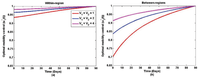
In the next simulation, cost functional weights $V_{1}$ and $V_{2}$ were changed, where the higher weights influence more contraction on $(1 - u_{j} (t))^{2}$ ; $j = 1, 2$ in the minimization process. Such a contraction allows $u_{j} (t)$ to increase, which guides the relaxation of mobility restrictions. These behaviors can be verified by Figure 9. Here also, mobility restrictions between regions are higher than those within regions. By varying the weights, one can prioritize whether to minimize infected proportion or mobility restriction, and importantly, at which levels too.

Figure 9.

Variation of the infected proportions and optimal mobility controls for different cost functional weights $V_{1}$ and $V_{2}$ . The parameters are provided in Table 1 and in the subsection 2.5. The weights of the cost functional are $W_{1} = W_{2} = W_{3} = 100$ .

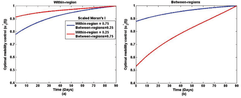
The next experiment reveals the mobility controls when within-region and between-region assignments are given different spatial variations. It is possible that a region is responsible for a clustering effect, but when coupled with another region, the total area may exhibit a dispersion effect. In Figure 10, the case shown in blue investigates such a scenario (scaled Moran’s $I$ : within-region = 0.75, between-region = 0.25)( $u_{1} \approx 0.78$ and $u_{2} \approx 0.88$ ). Contrastingly, the case in red illustrates dispersion for within-region and clustering for between-regions ( $u_{1} \approx 0.9$ and $u_{2} \approx 0.54$ ). In practice, this situation might occur when neighboring spatial units of different regions possess similar observations (High-High or Low-Low). According to Figure 10, higher mobility restrictions are also required in a contrasting way, again emphasizing more restrictions for clustering effect ( $u_{1} \approx 0.65$ and $u_{2} \approx 0.43$ ).

Figure 10.

Variation of the infected proportions and optimal mobility controls for different scaled Moran’s $I$ values representing within-region and between-region spatial effects. The parameters are provided in Table 1 and in the subsection 2.5. The weights of the cost functional are $W_{1} = W_{2} = W_{3} = 100$ and $V_{1} = V_{2} = 1$ .

More numerical experiments can be conducted using different combinations of spatial variations and cost functional weights. In a further study for Sri Lanka, one can categorize the regions with much smaller spatial units than districts, such as Medical Officer of Health (MOH) areas or local municipalities (Ganegoda et al., 2023, 2022). In such cases, distance-based weights $w_{i j}$ of Moran’s $I$ would be preferred. That would also enhance the statistical significance of Moran’s $I$ . Moreover, parameters directly involved in the dynamics (e.g., transmission rate $β$ , recovery rate $γ$ , etc.) can also be adjusted for testing different scenarios in various study areas, observation periods, or even for different diseases. Policymakers can also test different time frames, considering plausible social or economic constraints.

5. Discussion

The robustness and applicability of the proposed strategies are demonstrated through both stability and optimal control analyses. The stability analysis (3.2) shows how variations in infected proportions affect overall dynamics under different levels of spatial autocorrelation, while the optimal control analysis (4.3) incorporates region-specific differences using scaled Moran’s $I$ and cost functional weight. Together, these analyses illustrate how region-specific mobility controls can be designed under a range of plausible epidemic and mobility scenarios, highlighting the robustness, generalizability, and practical relevance of the proposed methodology.

The main tactic of this study was to introduce spatial autocorrelation measured by Moran’s $I$ into optimal mobility control. Three types of spatial variations were assimilated as clustering, dispersion, and random effects through parameters $k_{i j}$ referred to as scaled-Moran’s $I$ . Several numerical experiments were conducted by infusing scaled-Moran’s $I$ into the usual mobility patterns given by $m_{i j}$ .

Our two-way investigation contains a stability analysis and an optimal control analysis. The local stability analysis facilitates the understanding of the long-term infected proportion subject to the so-called self-control of human mobility. It means that people mobilize as they wish with no significant control by the government. This scenario aligned with the time period covered by the data in this case study, and the stability analysis was performed assuming such a mobility behavior prevails. Here, the whole country was considered as one spatial unit. As a preliminary finding, the basic reproduction number ( $R_{k}$ ) reduced as a result of Moran-induced mobility control, which is a usual observation in such controlled dynamics (Onah et al., 2022). Furthermore, the bifurcation analysis illustrated a forward behavior guaranteeing one stable endemic equilibrium level for the infected proportion that decreases when $R_{k}$ decreases (Cheneke, 2023). Unlike in the backward bifurcation, this would be preferable for control policies with a targeted intervention (Dushoff et al., 1998). Disease dynamics and the reproduction number can be changed by different variants with varying transmissibility ( $β$ ), and model accuracy can be improved by incorporating variant-specific transmissibility, which provides a valuable direction for future research.

Theorem 1 and Theorem 2 address necessary and sufficient conditions of self-control ( $u$ ) to achieve stable equilibria, both disease-free and endemic. The aim of these results is to identify at which level $u$ should be maintained for stability, taking spatial variations via the scaled-Moran’s $I$ also into account. Accordingly, a higher clustering effect recommends a lower upper bound on $u$ , suggesting more mobility restrictions. This outcome is important in practice since unstable chaotic behaviors of infected proportions would occur otherwise (Ganegoda & Perera, 2023; Sapkota et al., 2021). At times, oscillatory behaviors are possible, again hinting at non-stationary scenarios. However, as a further illustration, the Corollary 1 shows the bounds on $u$ to ensure damping oscillations leading to a stable equilibrium.

Government intervention is required for reliable control of disease transmission, despite some self-control achieved by following health guidelines such as wearing face masks, maintaining social distance, and using hand wash (Chiu et al., 2020; Güner et al., 2020). Meanwhile, the country should be open for usual economic activities amidst the risk of further escalations, which is always a challenging decision (Fu et al., 2022). As a compromised target, the overall risk of losing economy and escalating infected proportion should be minimized, subject to the disease transmission dynamics. Such an intervention should be planned and tested with a specific time bound, too. Catering to all these aspects, an optimal control analysis was carried out again, highlighting the spatial variations.

Mobility control was tailored with two approaches, within the region and between regions, for the specified three regions. Since a countrywide optimal plan was the focus, no direct region-wise controls were designed. However, region-specific attributes were absorbed into the model via scaled Moran’s $I$ parameters. Thus, $k_{i i} u_{1} (t)$ reflects within-region control of the Region $i$ while $k_{i j} u_{2} (t)$ stands for between-regions control relevant to Region $i$ and Region $j$ . For instance, a control level given by $u_{1} (t) = 0.8$ is assimilated as Moran-induced mobility control levels as $0.0784, 0.168$ , and $0.56$ for Region 1, Region 2, and Region 3, respectively. The same sort of argument can be established for $u_{2} (t)$ as well. This highlights the applicability of $k_{i j}$ in addressing spatial variations in clustering, dispersion, and random effects. Several cases with such variations were simulated in subsection 4.3 in which more mobility restrictions were indicated for clustering compared to dispersion. In practice, those restrictions may range from social distancing to travel restrictions and finally to a full lockdown of a country. More numerical experiments are possible by changing $k_{i j}$ . Such experiments demonstrate the applicability of $k_{i j}$ as a general technique of spatial analysis in disease transmission or in similar space-related dynamics.

It is also worthwhile to distinguish mobility control according to different government interests. More mobility restrictions lead to increased losses in earnings, which indirectly forces the government to spend on welfare activities as well (The World Bank, 2021a). Accordingly, some countries attempted to keep the country open with minimal effort on mobility control, while in others, although controls were implemented, the level of imposing mobility restrictions varied (Rahman & Thill, 2022; Yao et al., 2022). In our analysis, such consequences can be mitigated by adjusting the weights in the cost functional (10). As a basic move, comparatively different values were set for the two categories of weights mapping the cost of infected proportions ( $W_{1}, W_{2}$ and $W_{3}$ ) and the cost of mobility control ( $V_{1}$ and $V_{2}$ ). Lower $V_{1}$ and $V_{2}$ values incorporate lesser interest on mobility control (see Figure 9).

There are a few additional aspects to consider in terms of the model’s general outlook and calibration used here. The parameter $Λ$ , called recruitment rate, has been introduced, overwriting the usual birth rate as input source for the long run. In a highly transmissible disease such as COVID-19, it is reasonable to estimate input rates of the susceptible compartment by fitting data, rather than relying on a census figure of the birth rate. Moreover, the removal rate ( $μ$ ) was also set to match that of $Λ$ compiling removals due to immunity, vaccination, and deaths. Usual mobility rates were calculated using the gravity model, where different methods, such as the radiation model or combined versions, are also possible (Barbosa et al., 2018). Utilizing human mobility data collected in the field is the ideal approach, but it is often limited in availability and accessibility (Oliver et al., 2024). In computing Moran’s $I$ , the adjacency weights were used. There are more versions, such as distance-based weights, when a higher degree of spatial connectivity needs to be captured (Ganegoda et al., 2023). This was not attempted in our case, as the focus was on deriving an optimal control strategy that considered simple mobility across neighboring districts. In solving the optimal control problem, the standard Hamiltonian process was implemented in accordance with Pontryagin’s Maximum Principle (Appendix 7). Convexity of the Hamiltonian function over control variables ensures the existence of an optimal solution (Lee & Castillo-Chavez, 2015). Our optimal controls were technically bounded in $(0, 1]$ , and it can be tolerated to any interval $[a, b] \subseteq (0, 1]$ to assimilate field observations. For instance, one can choose such a $[a, b]$ interval if there is sufficient evidence that full open or full lockdown states are not feasible. The theoretical and computational techniques proposed in this work are readily open for further improvements.

This study is based on simplified assumptions to illustrate the effects of spatial variations and mobility control on disease spread. The results provide rough guidance and insights for policy considerations, but such guidance should be tested at the community level for official public health decisions.

6. Conclusion

The clustering effect of disease incidence demonstrates a high risk of transmission, in contrast to the dispersion effect. The availability of Moran-induced parameters in epidemic models facilitates more in-depth analysis of spatial variations, along with authentic adaptation to different study areas. Here the applicability of Moran’s $I$ statistic is emphasized. Stable disease-free and endemic equilibria can be achieved, but with severe restrictions on human mobility, which is often not attainable without the intervention of the governments. These facts have been tested for COVID-19 in this study, filling the literature gap of incorporating spatial autocorrelation into optimal control models. By such an approach, health authorities can successfully minimize the number of infected cases while allowing the country to remain open for normal socio-economic activities. The dilemma of when and where to relax mobility restrictions and at which level can be curbed by testing with different spatial variations, as proposed in this work.

Footnotes

ORCID iDs

Ahangama Vithanage Ravindu Hansana

Naleen Chaminda Ganegoda

Hemamali Chathurangani Yashika Jayathunga

Funding

The author(s) received no financial support for the research, authorship and/or publication of this article.

Declaration of Conflicting Interests

The authors declared no potential conflicts of interest with respect to the research, authorship, and/or publication of this article.

Data Availability Statement

COVID-19 data were retrieved from the Epidemiology Unit of the Ministry of Health, Sri Lanka ().

Appendix A

The Hamiltonian of the control system (9) can be obtained as follows. (13)

\begin{aligned} H & = \sum_{i = 1}^{3} W_{i} I_{i} (t) + \sum_{j = 1}^{2} V_{j} (1 - u_{j} (t))^{2} \\ + λ_{1} [Λ - β S_{1} (k_{11} u_{1} (t) m_{11} I_{1} + k_{12} u_{2} (t) m_{12} I_{2} + k_{13} u_{2} (t) m_{13} I_{3}) - μ S_{1}] \\ + λ_{2} [β S_{1} (k_{11} u_{1} (t) m_{11} I_{1} + k_{12} u_{2} (t) m_{12} I_{2} + k_{13} u_{2} (t) m_{13} I_{3}) - I_{1} (γ + μ)] \\ + λ_{3} [γ I_{1} - μ R_{1}] \\ + λ_{4} [Λ - β S_{2} (k_{22} u_{1} (t) m_{22} I_{2} + k_{12} u_{2} (t) m_{12} I_{1} + k_{23} u_{2} (t) m_{23} I_{3}) - μ S_{2}] \\ + λ_{5} [β S_{2} (k_{22} u_{1} (t) m_{22} I_{2} + k_{12} u_{2} (t) m_{12} I_{1} + k_{23} u_{2} (t) m_{23} I_{3}) - I_{2} (γ + μ)] \\ + λ_{6} [γ I_{2} - μ R_{2}] \\ + λ_{7} [Λ - β S_{3} (k_{33} u_{1} (t) m_{33} I_{3} + k_{13} u_{2} (t) m_{13} I_{1} + k_{23} u_{2} (t) m_{23} I_{2}) - μ S_{3}] \\ + λ_{8} [β S_{3} (k_{33} u_{1} (t) m_{33} I_{3} + k_{13} u_{2} (t) m_{13} I_{1} + k_{23} u_{2} (t) m_{23} I_{2}) - I_{3} (γ + μ)] \\ + λ_{9} [γ I_{3} - μ R_{3}] \end{aligned}

There exist optimal controls $U^{*} (t) = (u_{1}^{*} (t), u_{2}^{*} (t))$ and corresponding state solutions that minimize $J (U)$ . In order for the above statement to be true, it is necessary that there exist continuous functions $λ_{i} (t); i = 1, 2, . ., 9$ such that, (14)

\begin{aligned} \frac{\partial λ_{1}}{\partial t} & = - \frac{\partial H}{\partial S_{1}} = (λ_{1} - λ_{2}) (k_{11} u_{1} m_{11} β I_{1} + k_{12} u_{2} m_{12} β I_{2} + k_{13} u_{2} m_{13} β I_{3}) + λ_{1} μ \\ \frac{\partial λ_{2}}{\partial t} & = - \frac{\partial H}{\partial I_{1}} = - w_{1} + (λ_{1} - λ_{2}) k_{11} u_{1} m_{11} β S_{1} + (λ_{4} - λ_{5}) k_{12} u_{2} m_{12} β S_{2} \\ + (λ_{7} - λ_{8}) k_{13} u_{2} m_{13} β S_{3} - (λ_{3} - λ_{2}) γ + λ_{2} μ \\ \frac{\partial λ_{3}}{\partial t} & = - \frac{\partial H}{\partial R_{1}} = λ_{3} μ \\ \frac{\partial λ_{4}}{\partial t} & = - \frac{\partial H}{\partial S_{2}} = (λ_{4} - λ_{5}) (k_{22} u_{1} m_{22} β I_{2} + k_{12} u_{2} m_{12} β I_{1} + k_{23} u_{2} m_{23} β I_{3}) + λ_{4} μ \\ \frac{\partial λ_{5}}{\partial t} & = - \frac{\partial H}{\partial I_{2}} = - w_{2} + (λ_{1} - λ_{2}) k_{12} u_{2} m_{12} β S_{1} + (λ_{4} - λ_{5}) k_{22} u_{1} m_{22} β S_{2} \\ + (λ_{7} - λ_{8}) k_{23} u_{2} m_{23} β S_{3} - (λ_{6} - λ_{5}) γ + λ_{5} μ \\ \frac{\partial λ_{6}}{\partial t} & = - \frac{\partial H}{\partial R_{2}} = λ_{6} μ \\ \frac{\partial λ_{7}}{\partial t} & = - \frac{\partial H}{\partial S_{3}} = (λ_{7} - λ_{8}) (k_{33} u_{1} m_{33} β I_{3} + k_{13} u_{2} m_{13} β I_{1} + k_{23} u_{2} m_{23} β I_{2}) + λ_{7} μ \\ \frac{\partial λ_{8}}{\partial t} & = - \frac{\partial H}{\partial I_{3}} = - w_{3} + (λ_{1} - λ_{2}) k_{13} u_{2} m_{13} β S_{1} + (λ_{4} - λ_{5}) k_{23} u_{2} m_{23} β S_{2} \\ + (λ_{7} - λ_{8}) k_{33} u_{1} m_{33} β S_{3} - (λ_{9} - λ_{8}) γ + λ_{8} μ \\ \frac{\partial λ_{9}}{\partial t} & = - \frac{\partial H}{\partial R_{3}} = λ_{9} μ . \end{aligned}

Furthermore, the transversality conditions can be written as $λ_{i} (t_{f}) = 0; i = 1, 2, . ., 9$ .

The optimal control variable can be obtained as follows using the optimality condition $\frac{\partial H}{\partial u_{i}} = 0; i = 1, 2$ (Lee & Castillo-Chavez, 2015; Lenhart & Workman, 2007).

(15)

\begin{aligned} u_{1}^{*} & = min {b_{1}, max {a_{1}, \frac{2 V_{1} + (λ_{1} - λ_{2}) k_{11} m_{11} β S_{1} I_{1} + (λ_{4} - λ_{5}) k_{22} m_{22} β S_{2} I_{2} + (λ_{7} - λ_{8}) k_{33} m_{33} β S_{3} I_{3}}{2 V_{1}}}}, \\ u_{2}^{*} & = min {b_{2}, max {a_{2}, \frac{P_{1} + P_{2} + P_{3}}{2 V_{2}}}}, \\ where P_{1} & = 2 V_{2} + (λ_{1} - λ_{2}) (k_{12} m_{12} β S_{1} I_{2} + k_{13} m_{13} β S_{1} I_{3}), \\ P_{2} & = (λ_{4} - λ_{5}) (k_{12} m_{12} β S_{2} I_{1} + k_{23} m_{23} β S_{2} I_{3}), \\ P_{3} & = (λ_{7} - λ_{8}) (k_{13} m_{13} β S_{3} I_{1} + k_{23} m_{23} β S_{3} I_{2}) . \end{aligned}

References

Abdulhafedh

(2017). A novel hybrid method for measuring the spatial autocorrelation of vehicular crashes: Combining Moran’s index and Getis-Ord Gi statistic. Open Journal of Civil Engineering, 7, 208–221. https://doi.org/10.4236/ojce.2017.72013

Adepoju

O. A.

Olaniyi

(2021). Stability and optimal control of a disease model with vertical transmission and saturated incidence. Scientific African, 12, e00800. https://doi.org/10.1016/j.sciaf.2021.e00800

Aldila

Götz

Soewono

(2013). An optimal control problem arising from a dengue disease transmission model. Mathematical Biosciences, 242(1), 9–16. https://doi.org/10.1016/j.mbs.2012.11.014

Amaratunga

Fernando

Haigh

Jayasinghe

(2020). The COVID-19 outbreak in Sri Lanka: A synoptic analysis focusing on trends, impacts, risks and science-policy interaction processes. Progress in Disaster Science, 8, 100133. https://doi.org/10.1016/j.pdisas.2020.100133

Andrews

M. R.

Tamura

Best

J. N.

Ceasar

J. N.

Batey

K. G.

Kearse

T. A.

Allen

L. V.

Baumer

Collins

B. S.

Mitchell

V. M.

Powell-Wiley

T. M.

(2021). Spatial clustering of county-level COVID-19 rates in the US. International Journal of Environmental Research and Public Health, 18(22), 12170. https://doi.org/10.3390/ijerph182212170

Anselin

(1996). The Moran scatterplot as an ESDA tool to assess local instability in spatial association. In M. M. Fischer, H. J. Scholten, & D. J. Unwin (Eds.), Spatial Analytical Perspectives on GIS (pp. 111–125). London: Taylor & Francis.

Anselin

(2020). Global spatial autocorrelation. Retrieved 03.01.2022 from geodacenter.github.io

Central Bank of Sri Lanka. (2020). Annual report 2020. Retrieved August 20, 2021, from www.cbsl.gov.lk

Barbosa

Barthelemy

Ghoshal

James

C. R.

Lenormand

Louail

Menezes

Ramasco

J. J.

Simini

Tomasini

(2018). Human mobility: Models and applications. Physics Reports, 734, 1–74. https://doi.org/10.1016/j.physrep.2018.01.001

10.

Böck

Immitzer

Atzberger

(2017). On the objectivity of the objective function—problems with unsupervised segmentation evaluation based on global score and a possible remedy. Remote Sensing, 9, 769. https://doi.org/10.3390/rs9080769

11.

Boehmer

Harko

Sabau

(2010). Jacobi stability analysis of dynamical systems – applications in gravitation and cosmology. Advances in Theoretical and Mathematical Physics, 16. https://doi.org/10.4310/ATMP.2012.v16.n4.a2

12.

Bolzoni

Bonacini

Soresina

Groppi

(2017). Time-optimal control strategies in SIR epidemic models. Mathematical Biosciences, 292, 86–96. https://doi.org/10.1016/j.mbs.2017.07.011

13.

Chawla

S. R.

Ahmad

Khan

Albalawi

Nisar

K. S.

Ali

H. M.

(2024). Stability analysis and optimal control of a generalized SIR epidemic model with harmonic mean type of incidence and nonlinear recovery rates. Alexandria Engineering Journal, 97, 44–60. https://doi.org/10.1016/j.aej.2024.04.017

14.

Chen

(2013). New approaches for calculating Moran’s index of spatial autocorrelation. PloS one, 8(7), e68336. https://doi.org/10.1371/journal.pone.0068336

15.

Chen

(2021). An Analytical Process of patial autocorrelation functions based on Moran’s index. PloS one, 16(4), e0249589. https://doi.org/10.1371/journal.pone.0249589

16.

Cheneke

(2023). Forward bifurcation and stability analysis. https://doi.org/10.5772/intechopen.112600

17.

Chiu

N. C.

Chi

Tai

Y. L.

Peng

C. C.

Tseng

C. Y.

Chen

C. C.

Tan

B. F.

Lin

C. Y.

(2020). Impact of wearing masks, hand hygiene, and social distancing on influenza, enterovirus, and all-cause pneumonia during the coronavirus pandemic: Retrospective national epidemiological surveillance study. Journal of Medical Internet Research, 22(8), e21257. https://doi.org/10.2196/21257 10.2196/21257

18.

Daily Mirror. (2021a). Inter-provincial travel ban further extended. Retrieved January 15, 2022, from www.dailymirror.lk

19.

Daily Mirror. (2021b). Travails of people in troubled times. Retrieved April 04, 2022, from www.dailymirror.lk

20.

Department of Census and Statistics - Sri Lanka. (2022). Population and housing. Retrieved March 20, 2022, from www.statistics.gov.lk

21.

Disselhorst

(2021). Optimal control of epidemics: Analysis of optimal government intervention, testing, and vaccination strategies (Master’s Thesis). University of Groningen.

22.

Zhao

Sun

(2021). Modelling the epidemic dynamics of COVID-19 with consideration of human mobility. International Journal of Data Science and Analytics, 12(4), 369–382. https://doi.org/10.1007/s41060-021-00271-3

23.

Dushoff

Huang

Castillo-Chávez

(1998). Backward bifurcations and catastrophe in simple models of fatal diseases. Journal of Mathematical Biology, 36, 227–248. https://doi.org/10.1007/s002850050099

24.

Economynext. (2021). Sri lanka’s COVID-19 inter-province travel ban to be strictly enforced till Oct 21. Accessed: 2024-12-24.

25.

Epidemiology Unit – Ministry of Health Sri Lanka. (2021). COVID-19 daily situation report. Retrieved December 15, 2022, from www.epid.gov.lk/web/index.php?option=com_content&view=article&id=225&lang=en

26.

Franch-Pardo

Napoletano

B. M.

Rosete-Verges

Billa

(2020). Spatial analysis and GIS in the study of COVID-19: A review. Science of The Total Environment, 739, 140033. https://doi.org/10.1016/j.scitotenv.2020.140033

27.

Jin

Xiang

Wang

(2022). Optimal lockdown policy for vaccination during COVID-19 pandemic. Finance Research Letters, 45, 102123. https://doi.org/10.1016/j.frl.2021.102123

28.

Fudolig

Howard

(2020). The local stability of a modified multi-strain SIR model for emerging viral strains. PloS one, 15(12), e0243408. https://doi.org/10.1371/journal.pone.0243408

29.

Ganegoda

N. C.

Aldila

Wijaya

K. P.

(2023). Spatiotemporal dynamics of disease transmission: Learning from COVID-19 data. In M. Vithanage & M. N. V. Prasad (Eds.), Sustainable Approaches in Environmental Science: Learning from COVID-19 Pandemic, chapter 13. Wiley. https://doi.org/10.1002/9781119867333.ch13.

30.

Ganegoda

N. C.

Perera

S. S. N.

(2023). Chaos of COVID-19 superspreading events: An analysis via a data-driven approach. Journal of Health Management, 25(3), 514–525. https://doi.org/10.1177/09720634221150964

31.

Ganegoda

N. C.

Wijaya

K. P.

Chávez

J. P.

Aldila

Erandi

K. K. W. H.

Amadi

(2022). Reassessment of contact restrictions and testing campaigns against COVID-19 via spatio-temporal modeling. Nonlinear Dynamics, 107(3), 3085–3109. https://doi.org/10.1007/s11071-021-07111-w

32.

Getis

Ord

J. K.

(1992). The analysis of spatial association by use of distance statistics. Geographical analysis, 24(3), 189–206. https://doi.org/10.1111/j.1538-4632.1992.tb00261.x

33.

Getis

Ord

J. K.

(1995). Local spatial autocorrelation statistics: distributional issues and an application. Geographical analysis, 27(4), 286–306. https://doi.org/10.1111/j.1538-4632.1995.tb00912.x

34.

Guckenheimer

Holmes

(2013). Nonlinear oscillations, dynamical systems, and bifurcations of vector fields. Applied Mathematical Sciences. Springer New York.

35.

Güner

Hasanoğlu

Aktaş

(2020). COVID-19: Prevention and control measures in community. Turkish Journal of Medical Sciences, 50(SI-1), 571–577. https://doi.org/10.3906/sag-2004-146

36.

Hale

J. K.

(1969). Dynamical systems and stability. Journal of Mathematical Analysis and Applications, 26(1), 39–59. https://doi.org/10.1016/0022-247X(69)90175-9

37.

Han

Yang

Jia

Feng

Chen

Zhao

Pereira

(2021). Spatial distribution characteristics of the COVID-19 pandemic in beijing and its relationship with environmental factors. Science of The Total Environment, 761, 144257. https://doi.org/10.1016/j.scitotenv.2020.144257

38.

Hansana

Ganegoda

Jayathunga

(2024). Optimal control strategies on mobility for preventing COVID-19 transmission: A study with a three-patch compartmental model. Communication in Biomathematical Sciences, 7(1), 34–49. https://doi.org/10.5614/cbms.2024.7.1.2

39.

Hong

Jung

W. S.

H. H.

(2019). Gravity model explained by the radiation model on a population landscape. PloS one, 14(6), e0218028. https://doi.org/10.1371/journal.pone.0218028

40.

Jackson

M. C.

Huang

Xie

Tiwari

R. C.

(2010). A modified version of Moran’s I. International Journal of Health Geographics, 9(1), 33. https://doi.org/10.1186/1476-072X-9-33

41.

Khan

A. A.

Ullah

Amin

(2022). Optimal control analysis of COVID-19 vaccine epidemic model: A case study. The European Physical Journal Plus, 137, 156. https://doi.org/10.1140/epjp/s13360-022-02365-8

42.

Kjellesvig

Atique

Böcker

Aamodt

(2025). Association between urban green space and transmission of COVID-19 in oslo, norway: A bayesian sir modeling approach. Spatial and Spatio-temporal Epidemiology, 52, 100699. https://doi.org/10.1016/j.sste.2024.100699

43.

Lan

Delmelle

(2023). Space-time cluster detection techniques for Infectious Diseases: A systematic review. Spatial and Spatio-temporal Epidemiology, 44, 100563. https://doi.org/10.1016/j.sste.2022.100563

44.

Lee

K. S.

Eom

J. K.

(2024). Systematic literature review on impacts of COVID-19 pandemic and corresponding measures on mobility. Transportation, 51(5), 1907–1961. https://doi.org/10.1007/s11116-023-10392-2

45.

Lee

Castillo-Chavez

(2015). The role of residence times in two-patch dengue transmission dynamics and optimal strategies. Journal of Theoretical Biology, 374, 152–164. https://doi.org/10.1016/j.jtbi.2015.03.005

46.

Lee

S. I.

(2017). Correlation and spatial autocorrelation. Springer International Publishing. (pp. 360–368). https://doi.org/10.1007/978-3-319-17885-1_1524

47.

Lenhart

Workman

J. T.

(2007). Optimal control applied to biological models. CRC press.

48.

Liu

Wang

Zhong

Zhang

Luo

Zhang

(2024). Spatiotemporal changes and influencing factors of hand, foot, and mouth disease in Guangzhou, China, from 2013 to 2022: Retrospective analysis. JMIR Public Health and Surveillance, 10, e58821. https://doi.org/10.2196/58821

49.

Liu

Song

Zhu

Tian

Gao

Zhang

Shao

Liu

Lin

(2020a). Population movement, city closure in Wuhan, and geographical expansion of the COVID-19 infection in China in january 2020. Clinical Infectious Diseases, 71(16), 2045–2051. https://doi.org/10.1093/cid/ciaa422

50.

Liu

Wang

Ren

Tian

Zhou

Zhao

Qiu

(2020b). A COVID-19 risk assessment decision support system for general practitioners: Design and development study. Journal of Medical Internet Research, 22(6), e19786. https://doi.org/10.2196/19786

51.

Zhu

Liu

Luo

Zhang

(2022). Spatial patterns of the spread of COVID-19 in singapore and the influencing factors. ISPRS International Journal of Geo-Information, 11(3). https://doi.org/10.3390/ijgi11030152

52.

Martcheva

(2015). An introduction to mathematical epidemiology. Springer.

53.

Massachusetts Institute of Technology (2020). Vida decision support system for COVID-19. www.media.mit.edu

54.

Michel

A. N.

Hou

Liu

(2015). Stability of dynamical systems: On the role of monotonic and non-monotonic Lyapunov Functions. Springer.

55.

Mohajan

(2022). Mathematical analysis of SIR model for COVID-19 transmission. Journal of Innovations in Medical Research, 1(2), 1–18. https://doi.org/10.56397/JIMR/2022.09.01

56.

Moran

P. A. P.

(1948). The interpretation of statistical maps. Journal of the Royal Statistical Society B, 10, 243–251. https://doi.org/10.1111/j.2517-6161.1948.tb00012.x

57.

Nepomuceno

E. G.

Peixoto

M. L. C.

Lacerda

M. J.

Campanharo

A. S. L. O.

Takahashi

R. H. C.

Aguirre

L. A.

(2021). Application of optimal control of infectious diseases in a model-free scenario. SN Computer Science, 2(5), 405. https://doi.org/10.1007/s42979-021-00794-3

58.

Nur

Rachman

Abdal

N. M.

Abdy

Side

(2018). SIR model analysis for transmission of dengue fever disease with climate factors using Lyapunov Function. Journal of Physics: Conference Series, 1028(1), 012117. https://doi.org/10.1088/1742-6596/1028/1/012117

59.

Oka

Wei

Zhu

(2021). The effect of human mobility restrictions on the COVID-19 transmission network in China. PloS one, 16(7), e0254403. Retrieved January 15, 2022, from. https://doi.org/10.1371/journal.pone.0254403

60.

Oliver

R. Y.

Chapman

Ellis-Soto

Brum-Bastos

Cagnacci

Long

Loretto

M. C.

Patchett

Rutz

(2024). Access to human-mobility data is essential for building a sustainable future. Cell Reports Sustainability, 1(4), 100077. https://doi.org/10.1016/j.crsus.2024.100077

61.

Onah

I. S.

Aniaku

S. E.

Ezugorie

O. M.

(2022). Analysis and optimal control measures of diseases in cassava population. Optimal Control Applications and Methods. https://doi.org/10.1002/oca.2901

62.

Petronilla

O. U.

Avurake

O. M.

Ifeyinwa

M. H.

(2017). Comparison between measures of spatial autocorrelation. International Journal of Mathematics and Statistics Invention (IJMSI), 5(9), 01–12.

63.

Pfeiffer

D. U.

Robinson

T. P.

Stevenson

Stevens

K. B.

Rogers

D. J.

Clements

A. C. A.

(2008). Spatial analysis in epidemiology. Oxford University Press. ISBN 9780198509882. https://doi.org/10.1093/acprof:oso/9780198509882.001.0001

64.

Rahman

M. M.

Thill

J. C.

(2022). Associations between COVID-19 pandemic, lockdown measures and human mobility: Longitudinal evidence from 86 countries. International Journal of Environmental Research and Public Health, 19(12), 7317. https://doi.org/10.3390/ijerph19127317

65.

Rendana

Idris

W. M. R.

Abdul Rahim

(2021). Spatial distribution of COVID-19 cases, epidemic spread rate, spatial pattern, and its correlation with meteorological factors during the first to the second waves. Journal of Infection and Public Health, 14(10), 1340–1348. Special Issue on COVID-19 – Vaccine, Variants and New Waves. https://doi.org/10.1016/j.jiph.2021.07.010

66.

Salman

A. M.

Mohd

M. H.

Muhammad

(2023). A novel approach to investigate the stability analysis and the dynamics of reaction–diffusion SVIR epidemic model. Communications in Nonlinear Science and Numerical Simulation, 126, 107517. https://doi.org/10.1016/j.cnsns.2023.107517

67.

Sapkota

Karwowski

Davahli

M. R.

et al (2021). The chaotic behavior of the spread of infection during the COVID-19 pandemic in the united states and globally. IEEE Access, 9, 80692–80702. https://doi.org/10.1109/ACCESS.2021.3085240

68.

Schmal

Myung

Herzel

Bordyugov

(2017). Moran’s I quantifies spatio-temporal pattern formation in neural imaging data. Bioinformatics (Oxford, England), 33(19), 3072–3079. https://doi.org/10.1093/bioinformatics/btx351

69.

Sigler

Mahmuda

Kimpton

Loginova

Wohland

Charles-Edwards

Corcoran

(2021). The socio-spatial determinants of COVID-19 diffusion: the impact of globalisation, settlement characteristics and population. Globalization and Health, 17(1), 56. https://doi.org/10.1186/s12992-021-00707-2

70.

Smith

T. E.

(2017). Spatial weight matrices. Retrieved March 03, 2021.

71.

Sri Lanka Army (2021). New year cluster rises to 98,534 - nocpco. Retrieved December 13, 2024, from www.army.lk/news/new-year-cluster-rises-98534-nocpco

72.

Srinivasan

Shrestha

Harris

D. R.

Lewis

Rock

Silwal

Pustz

Barboza-Salerno

Stopka

T. J.

(2025). Employment industry and opioid overdose risk: A pre- and post-COVID-19 comparison in Kentucky and Massachusetts 2018–2021. Spatial and Spatio-temporal Epidemiology, 52, 100701. https://doi.org/10.1016/j.sste.2024.100701

73.

Stavroulakis

Bolzon

Waszczyszyn

Ziemianski

(2003). 3.13 - inverse analysis. In I. Milne, R. Ritchie, & B. Karihaloo (Eds.). Comprehensive Structural Integrity (pp. 685–718). Oxford: Pergamon. https://doi.org/10.1016/B0-08-043749-4/03117-7

74.

Sun

Xue

Xie

(2017). Spatial-temporal distribution of dengue and climate characteristics for two clusters in Sri Lanka from 2012 to 2016. Scientific Reports, 7(1), 12884. https://doi.org/10.1038/s41598-017-13163-z

75.

Sunday Times Editorial. (2021). New wave of covid-19: Critical time for sl. The Sunday Times, Sri Lanka Retrieved December 12, 2021, from www.sundaytimes.lk

76.

The World Bank. (2020). Sri Lanka’s COVID-19 response: Saving lives today, preparing for tomorrow. Retrieved June 06, 2021, from www.worldbank.org

77.

The World Bank. (2021a). Economic and poverty impact of COVID-19. Retrieved May 03, 2023.

78.

The World Bank. (2021b). Sri Lanka’s COVID-19 response: Saving lives today, preparing for tomorrow. Retrieved January 10, 2022.

79.

Wendell Fleming

R. R.

(1975). Deterministic and stochastic optimal control. Springer.

80.

Yamada

(2024). Moran’s I for multivariate spatial data. Mathematics, 12(17). https://doi.org/10.3390/math12172746

81.

Yao

Wang

Liu

(2022). Lockdown policies, economic support, and mental health: Evidence from the COVID-19 pandemic in united states. Frontiers in Public Health, 10, 857444. https://doi.org/10.3389/fpubh.2022.857444

82.

Yao

Shi

Zhang

Liu

Luo

(2021). Examining the diffusion of coronavirus disease 2019 cases in a metropolis: a space syntax approach. International Journal of Health Geographics, 20(1), 17. https://doi.org/10.1186/s12942-021-00270-4

83.

Zhou

Lin

(2008). Geary’s C. In S. Shekhar & H. Xiong (Eds.), Encyclopedia of GIS (pp. 329–330). Springer, Boston.