Parameter-optimization-based ECMS for plug-in hybrid electric buses considering driving cycle recognition

Abstract

An appropriate energy management strategy is crucial to achieving energy-saving and emission-reduction goals for plug-in hybrid electric buses (PHEB). This study proposes an adaptive equivalent consumption minimization strategy (A-ECMS) considering the driving cycle recognition based on the P2 configuration to achieve dynamic real-time adjustment of the equivalent factor (EF). First, local driving conditions are collected and preprocessed using an intelligent transportation system (ITS). Second, features are extracted from the speed window using the sliding window method, and an algorithm combining Particle Swarm Optimization and a Support Vector Machine (PSO-SVM) is used for driving cycle data classification prediction and relevant parameter optimization. Moreover, three key parameters-EF, the penalty factor, and the transmission ratio of the main reducer-are optimized using the Grey Wolf Optimizer (GWO) to reduce operating costs, and model simulations are conducted for verification. The comparison between the simulation results and the hardware-in-the-loop (HIL) test results shows that the proposed strategy can achieve excellent fuel economy, which is consistent with the expected results.

Keywords

plug-in hybrid electric bus driving cycle recognition equivalent consumption minimization strategy machine learning HIL test

Introduction

To address the global energy crisis and environmental pollution, hybrid electric vehicles (HEVs) have emerged as highly effective alternatives to replace traditional fuel vehicles.^1–4 The advancement of electrification and hybridization technologies has enabled the electric motor to become a primary power source, comparable to the internal combustion engine.^5,6 P2 configuration plug-in hybrid electric vehicles (PHEVs) have become the most popular hybrid configuration due to their ability to achieve better performance and fuel economy with minimal modifications.⁷ With the increasing recognition of new energy vehicles by the public, many new energy buses have also emerged in public transportation. Similar to how advanced motor control methods can improve the steady-state and transient performance of motors,⁸ an effective energy management strategy (EMS) can fully utilize the performance advantages of HEVs, improve fuel economy,^9,10 reduce operating costs, and enhance the service life of various components.

Due to the characteristics of multiple energy sources, an effective energy management strategy plays a vital role in the rational allocation of energy use in hybrid power systems.¹¹ Compared to rule-based strategies, optimization-based and learning-based control strategies have gained significant prominence in recent research. Optimization-based methods can be further divided into global optimization and instantaneous optimization approaches. Dynamic programming (DP) is a representative global optimization method; however, due to its discrete backward-solving nature and the curse of dimensionality, it is typically unsuitable for real-time online applications. On the other hand, Pontryagin’s Minimum Principle (PMP)¹² and equivalent consumption minimization strategy (ECMS)^13,14 are commonly used for instantaneous optimization. Instantaneous optimization approximates the cost function using rolling optimization and iterative methods to seek optimal control variables. For example,¹⁵ compared DP with PMP and ECMS while considering battery aging, reporting fuel consumption differences of 2.1% and 2.8%, respectively. Additionally,¹⁶ proposed an adaptive ECMS approach with neural network-trained shifting, which increased fuel consumption by only 3.23% compared to DP while significantly reducing computational effort. It is evident that different strategies are typically evaluated based on their proximity to DP in terms of effectiveness. Learning-based strategies have gradually become mainstream energy management strategies with the rise of artificial intelligence.¹⁷ Researchers often employ this strategy to predict vehicle states and learn optimal control behaviors.^18–21 Due to its high accuracy and strong adaptability, it exhibits significant advantages in highly nonlinear control scenarios.²² proposed a hierarchical control framework for HEVs by combining numerical optimization with deep learning, enabling real-time joint optimization of vehicle driving cycles and powertrain energy management.²³ innovatively utilized Q-learning to investigate the adaptability of supervised control for HEVs, demonstrating good fuel economy under different driving conditions. Meeting the increasingly diverse control requirements for HEVs proves challenging for a single control strategy. Various complex road conditions necessitate vehicles to possess adaptive capabilities, while ever-changing driving environments require vehicles to utilize internal and external information for online data prediction. This calls for control strategies that can integrate real-time data processing with computers. Moreover, addressing nonlinear optimization with multiple variables and constraints requires suitable methods. Therefore, there is a need to combine artificial intelligence with instantaneous optimization of vehicles to form a more efficient and precise control strategy.

The acquisition and processing of driving cycles fundamentally determine the distribution and control of internal energy in HEVs. The ability to obtain future driving cycle information in advance enables real-time online vehicle control, achieving near-DP global optimization performance. There are generally two methods for obtaining future driving cycle information:²⁴ utilizing established future speed prediction models based on historical vehicle speed data,^25–27 or collecting surrounding driving environment and traffic information through increasingly advanced intelligent transportation system (ITS)^28,29 and emerging technologies such as V2X.³⁰ With the support of driving cycle data, driving cycle classification recognition can be introduced to realize the adaptive control strategy and improve the sensitivity of driving conditions. For instance,³¹ divided driving cycles based on the actual station distribution of PHEBs and established a lookup table using the EF optimization results to achieve real-time online control. Zhang et al.³² proposed a novel A-ECMS by combining parameter optimization and driving cycle recognition while ensuring good fuel economy and stable battery state of charge (SOC). Considering that equivalent factor (EF) varies according to changes in the actual driving conditions, online ECMS strategies and driving cycle recognition predictions should be combined to further enhance the performance of ECMS under real driving conditions compared to its lower generality and real-time capability in offline ECMS.³³

This paper proposes an adaptive equivalent consumption minimization strategy (A-ECMS) based on driving cycle recognition and factor optimization. First, the local condition data is collected using the on-board speed testing system, and the actual condition of the bus in the city is obtained after preprocessing. Second, machine learning and intelligent algorithm are combined to classify and predict the driving cycle using the algorithm combined particle swarm optimization and support vector machine (PSO-SVM). Then, the balance between the actual SOC and the reference SOC is considered in the cost function to ensure that the battery energy is reduced to a lower limitation. Finally, grey wolf optimization (GWO) is used to optimize the three parameters, and the optimal control sequence is applied to the vehicle. The primary contributions of this paper are summarized as:

This paper proposes an innovative energy management strategy that integrates driving cycle recognition with parameter optimization, targeting the enhancement of fuel economy for plug-in hybrid electric buses across diverse road conditions. This approach addresses the issue of poor adaptability in energy management strategies under varying driving conditions.

Actual operational data from local urban bus routes were collected and a sample database was established based on both domestic and international standard operating conditions. Employing feature extraction techniques, the data were input into a Particle swarm optimization-Support vector machine model for training, enabling effective identification of driving cycles and providing valuable data resources for subsequent research.

The Grey Wolf Optimizer algorithm was applied to optimize selected parameters, with the outcomes reflected in three classified standard cycles, thereby further enhancing the effectiveness of the energy management strategy. Experimental validation demonstrated that, compared to traditional Equivalent Consumption Minimization Strategy and GWO-ECMS, the proposed strategy significantly reduces fuel consumption. Moreover, HIL testing indicated that this strategy can optimize torque distribution performance, demonstrating its potential for practical applications.

The remainder of this paper is organized as follows. Section II introduces the system model of P2 PHEB, which is the basis of subsequent simulation. Section III presents the driving cycle recognition and optimization algorithm in A-ECMS. In section IV, the theoretical results are simulated based on MATLAB/Simulink platform. Finally, conclusions are given in section V.

Hybrid system analysis and introduction

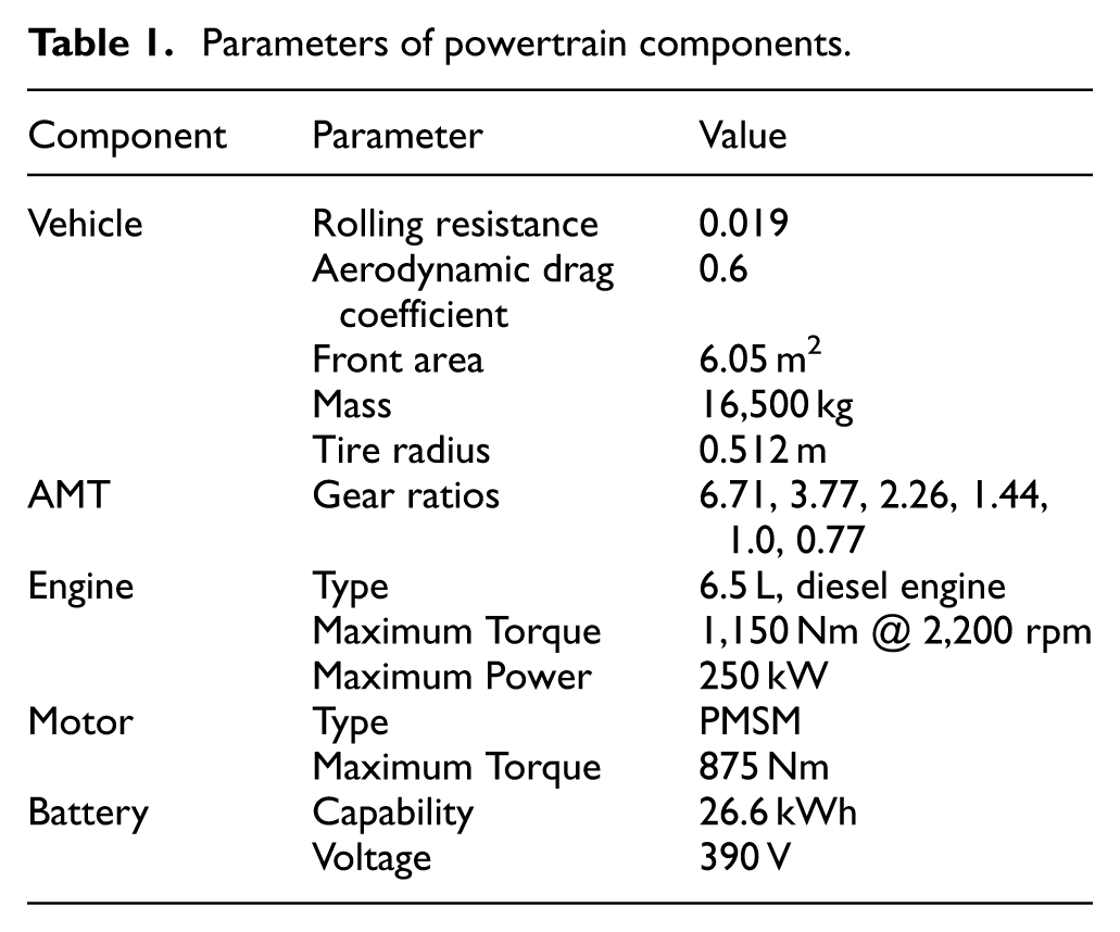
Currently, various configurations of hybrid electric buses exist worldwide. This study specifically focuses on the P2 configuration, as depicted in Figure 1. The P2 configuration adopts a coaxial parallel layout, incorporating an electric motor and a clutch between the engine and the AMT. A common drive shaft combines the power outputs of the engine and the electric motor. Typically, the electric motor functions as an auxiliary to the internal combustion engine, primarily providing additional power output and startup assistance. It can operate as both a motor and a generator, utilizing the stored electrical energy from the battery to power the vehicle, thereby reducing dependence on the internal combustion engine and enabling energy recuperation and fuel efficiency gains. The relevant parameters for the investigated PHEB are presented in Table 1.

Figure 1.

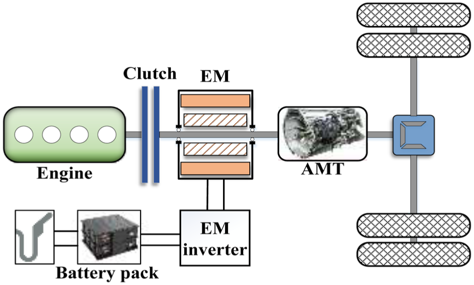
The architecture of the investigated PHEB.

Table 1.

Parameters of powertrain components.

Component	Parameter	Value
Vehicle	Rolling resistance	0.019
	Aerodynamic drag coefficient	0.6
	Front area	6.05 m²
	Mass	16,500 kg
	Tire radius	0.512 m
AMT	Gear ratios	6.71, 3.77, 2.26, 1.44, 1.0, 0.77
Engine	Type	6.5 L, diesel engine
	Maximum Torque	1,150 Nm @ 2,200 rpm
	Maximum Power	250 kW
Motor	Type	PMSM
Motor	Maximum Torque	875 Nm
Battery	Capability	26.6 kWh
Battery	Voltage	390 V

Vehicle longitudinal dynamics

The vehicle’s lateral dynamics and steering dynamics are typically analyzed to ensure handling stability and driving comfort. Fuel economy is typically the primary research objective in the energy management of PHEBs, which is fundamentally tied to the vehicle’s longitudinal dynamics. Therefore, this paper neglects lateral and steering dynamics and focuses exclusively on the longitudinal dynamic equation, expressed as follows:

F = {mgf}_{r} \cos θ + \frac{1}{2} C_{D} A_{f} ρ_{air} v_{a}^{2} + mg \sin θ + δ m \frac{{dv}_{a}}{dt}

(1)

where F is the driving force, f_r is the rolling resistance coefficient, C_D is the air resistance coefficient, and it is normally expressed as a function of Reynolds number, θ is the road gradient, A_f is the frontal area, ρ_air is the density of the air, δ is the vehicle rotation mass conversion coefficient, and v_a is the current vehicle speed.

Engine mathematical model

In the engine modeling of HEVs, it is usually not necessary to conduct a detailed investigation of the individual engine subsystems but rather treated it as integral parts of the overall system. Given the intricacy of the internal systems within an engine, this paper assumes it to be a perfect actuator capable of instantaneously responding to commands, thereby establishing a quasi-static engine model. For the engine, the instantaneous fuel consumption can be expressed as

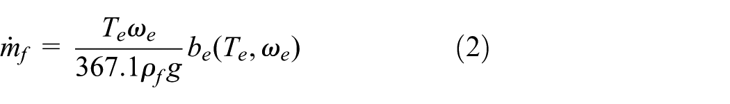
{\overset{\cdot}{m}}_{f} = \frac{T_{e} ω_{e}}{367.1 ρ_{f} g} b_{e} (T_{e}, ω_{e})

(2)

where T_e is the actual torque of the engine; ω_e is the rotational speed of the engine; ρ_f denotes the density of the fuel; b_e represents the fuel consumption rate.

EM mathematical model

The motor used in this paper is a permanent magnet synchronous motor (PMSM),^34–36 which can be modeled in a similar way to the engine, based on the PMSM efficiency map. The desired motor power or torque value can be used as a control input. Depending on whether it operates as a traction motor or a generator, the desired motor power can be mathematically expressed as follows:

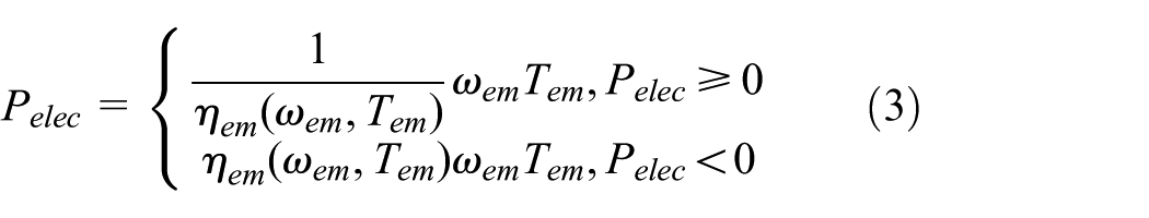
P_{elec} = {\begin{matrix} \frac{1}{η_{em} (ω_{em}, T_{em})} ω_{em} T_{em}, P_{elec} \geq 0 \\ η_{em} (ω_{em}, T_{em}) ω_{em} T_{em}, P_{elec} < 0 \end{matrix}

(3)

where P_elec is the electric power of the motor, T_em and ω_em are the torque and angular velocity of the motor, respectively; η_em can be obtained by the T_em and ω_em.

Battery model

Electrochemical energy storage systems, such as batteries and capacitors, play a crucial role in storing and recovering energy for powering electric motors. In vehicle simulators, the objective of battery models is typically to predict the variation of SOC under given electrical loads (Figure 2).

Figure 2.

The simplified diagram of the battery.

Considering that the number of battery parameters to be identified increases with the model order, this paper simplifies the battery model to an equivalent internal resistance model that only considers efficiency, while disregarding the dynamic characteristics of voltage. The SOC of the battery can be represented as follows:

I = \frac{Eb - \sqrt{{Eb}^{2} - 4 PbRb}}{2 Rb}

(4)

SOC = \frac{Qb - \int_{t 1}^{t 2} I dt}{Qb}

(5)

where I denotes the battery current, P_b, E_b, R_b, and Q_b represent the battery power, open-circuit voltage, internal resistance, and battery charge capacity, respectively. The variables t₁ and t₂ correspond to the start and end times, respectively. Notably, the SOC significantly affects the internal resistance and open-circuit voltage, which considerably impacts fuel economy. Experimental methods are primarily employed to quantify this relationship, as depicted in Figure 3.

Figure 3.

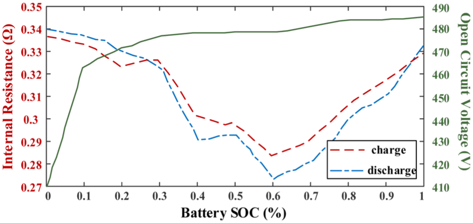
The schematic diagram of battery characteristics.

While the simplified equivalent internal resistance model is adopted in this study, it is worth qualitatively discussing the potential impacts of an advanced battery model. In reality, incorporating battery dynamics, temperature dependencies, and capacity aging could further improve the theoretical precision of the ECMS. For instance, temperature variations directly alter the internal resistance, thereby affecting the optimal equivalent factor; meanwhile, considering battery aging allows the strategy to balance instantaneous fuel economy against long-term battery degradation costs.³⁷ Furthermore, dynamic voltage limits can prevent over-current during sudden accelerations. However, integrating such advanced multi-physics models into online machine learning algorithms and real-time platforms inevitably introduces massive computational burdens and memory footprints. This severe computational overhead can lead to control latency, thereby compromising the real-time feasibility and responsiveness of the A-ECMS. Therefore, to ensure the real-time execution and control stability of the vehicle, the simplified macroscopic model is prioritized in this work as an optimal trade-off.

Energy management strategy and mode switching strategy

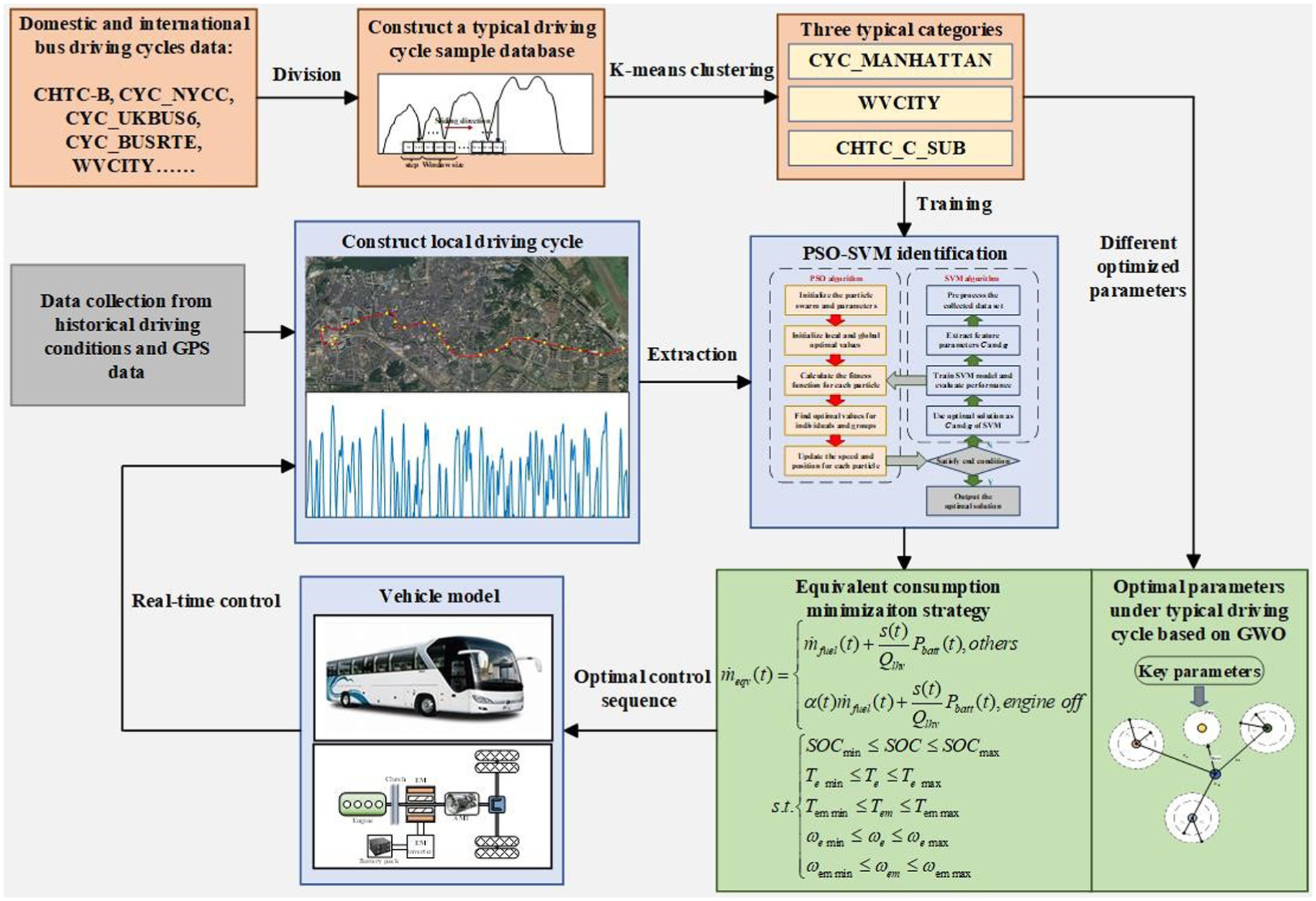
Driving cycle recognition is a technique based on vehicle data acquisition and analysis. It aims to identify the driving characteristics of HEVs under various conditions and optimize control strategies accordingly, thereby improving fuel economy and operational efficiency. The holistic control strategy block diagram is depicted in Figure 4.

Figure 4.

The proposed driving cycle recognition method.

Construction of local driving cycles and standard driving cycle database

To better evaluate the economy and practicability of the vehicle in real-world applications, this study utilizes the actual operational route of Bus Line 19 in a local city to represent the local driving conditions. This route is a representative operating line in the city, which is demonstrated in Figure 5. Its operation range includes a variety of different functional areas, such as commercial areas, residential neighborhoods, hospitals, schools, and railway stations, covering the smooth road conditions in the suburbs, the congested road conditions in the city center, and the complex and changeable road conditions at the station hub. This route’s operating hours span peak morning and evening periods, offering insights into the daily patterns of human mobility within the city. This system utilizes ground reference station differential data to achieve real-time carrier phase differential positioning, with a positioning accuracy of ±2 cm. Additionally, the integrated GPS navigation module within the system effectively provides real-time GPS data. The sampling frequency selected in the test is 1 Hz.

Figure 5.

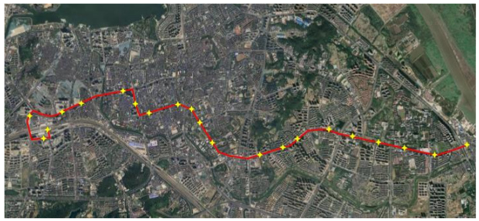
Testing route in the city.

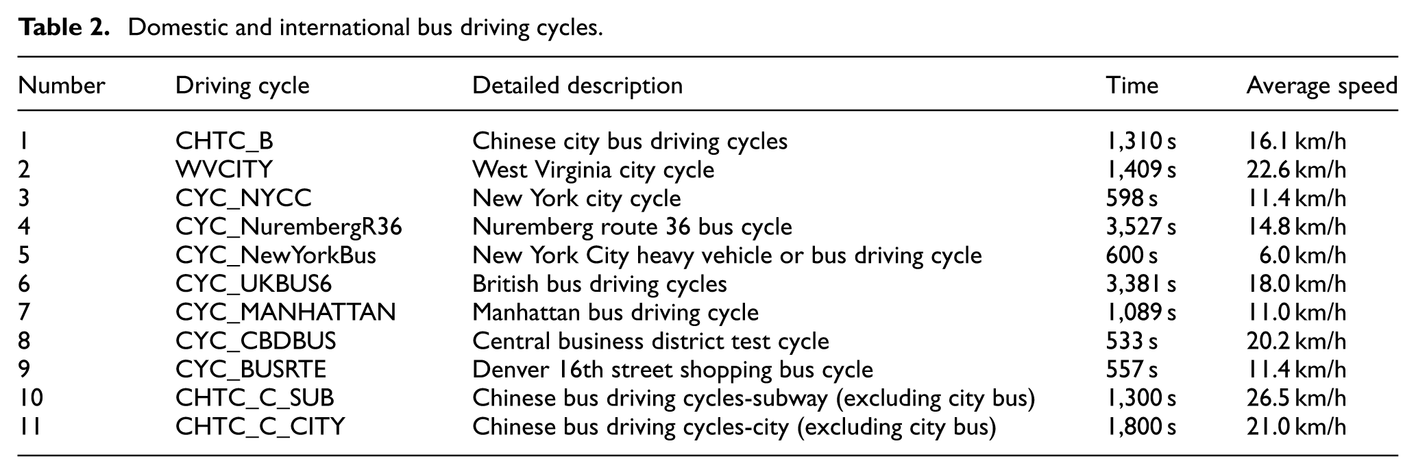
A fundamental step in implementing the driving cycle recognition algorithm is selecting an appropriate sample database; representative samples significantly enhance the robustness of the ECMS. The studied model of the paper focuses on the P2 hybrid electric bus, with operating routes primarily encompassing urban and suburban conditions within the city, excluding driving scenarios on highways. Therefore, a wide range of driving cycles from both domestic and international sources are extensively chosen to constitute the sample database, as indicated in Table 2.

Table 2.

Domestic and international bus driving cycles.

Number	Driving cycle	Detailed description	Time	Average speed
1	CHTC_B	Chinese city bus driving cycles	1,310 s	16.1 km/h
2	WVCITY	West Virginia city cycle	1,409 s	22.6 km/h
3	CYC_NYCC	New York city cycle	598 s	11.4 km/h
4	CYC_NurembergR36	Nuremberg route 36 bus cycle	3,527 s	14.8 km/h
5	CYC_NewYorkBus	New York City heavy vehicle or bus driving cycle	600 s	6.0 km/h
6	CYC_UKBUS6	British bus driving cycles	3,381 s	18.0 km/h
7	CYC_MANHATTAN	Manhattan bus driving cycle	1,089 s	11.0 km/h
8	CYC_CBDBUS	Central business district test cycle	533 s	20.2 km/h
9	CYC_BUSRTE	Denver 16th street shopping bus cycle	557 s	11.4 km/h
10	CHTC_C_SUB	Chinese bus driving cycles-subway (excluding city bus)	1,300 s	26.5 km/h
11	CHTC_C_CITY	Chinese bus driving cycles-city (excluding city bus)	1,800 s	21.0 km/h

The standard driving cycle is insufficient to support the required data for training the model. Therefore, the current paper adopts a sliding time window approach to divide the dataset. For each standard driving cycle, window size Δw and step Δs are set. As the window progressively moves from the starting point to the ending point with the step, a segment of data is formed for the kinematic features at each moment within the standard driving cycle, overcoming the problem of insufficient sample size. The schematic representation of the method is illustrated in Figure 6.

Figure 6.

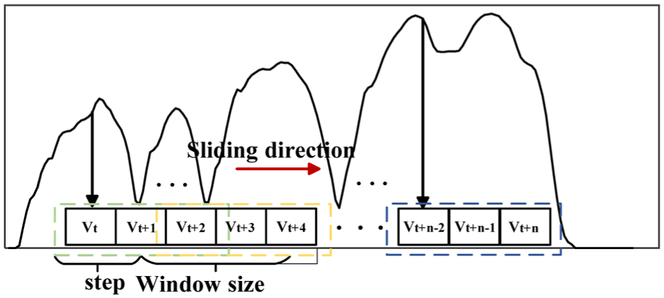
The schematic diagram of sliding time window.

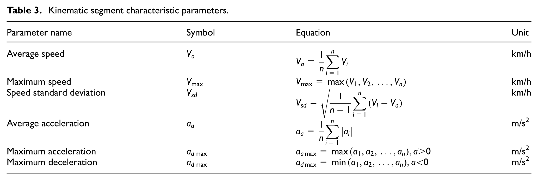
To better extract the kinematic segment features, this study selects six representative evaluation parameters from the 62 driving pattern parameters proposed in:^38,39 average speed V_a, maximum speed V_max, speed standard deviation V_sd, average acceleration a_a, maximum acceleration a_amax, and maximum deceleration a_dmax. The selection criteria for these six specific features are based on their strong correlation with the vehicle’s power demand and their ability to minimize data redundancy. Specifically, the speed-related parameters (V_a, V_max, V_sd) effectively reflect the steady-state load and overall kinetic energy, while the acceleration-related parameters (a_a, a_amax, a_dmax) characterize the transient dynamic demands and the potential for regenerative braking. Together, these six features can comprehensively and concisely depict the actual operating states of the bus without causing the curse of dimensionality during the algorithm training. The specific descriptions and formulas of these parameters are given in Table 3. In these equations, n represents the total number of sampling data points within a specific kinematic segment, i denotes the time index of the sampling point, V_i and a_i represent the instantaneous vehicle speed and acceleration at the ith sampling point, respectively.

Table 3.

Kinematic segment characteristic parameters.

Parameter name	Symbol	Equation	Unit
Average speed	$V_{a}$	$V_{a} = \frac{1}{n} \sum_{i = 1}^{n} V_{i}$	km/h
Maximum speed	$V_{max}$	$V_{max} = max (V_{1}, V_{2}, \dots, V_{n})$	km/h
Speed standard deviation	$V_{sd}$	$V_{sd} = \sqrt{\frac{1}{n - 1} \sum_{i = 1}^{n} (V_{i} - V_{a})}$	km/h
Average acceleration	$a_{a}$	$a_{a} = \frac{1}{n} \sum_{i = 1}^{n} \| a_{i} \|$	m/s²
Maximum acceleration	$a_{a max}$	$a_{a max} = max (a_{1}, a_{2}, \dots, a_{n}), a > 0$	m/s²
Maximum deceleration	$a_{d max}$	$a_{d max} = min (a_{1}, a_{2}, \dots, a_{n}), a < 0$	m/s²

Prior to being fed into the SVM model, these extracted features were verified using PCA and a Pearson correlation study. The analysis confirmed that the selected features exhibit minimal multi-collinearity and retain over 80% of the cumulative variance contribution of the original dataset, thereby ensuring computational efficiency and classification accuracy without requiring further high-dimensional feature reduction. The characteristic parameters of driving cycles in the sample database are calculated, and the 11 samples are divided into 3 categories in Table 4 by K-means clustering method, corresponding to three different road conditions in the local driving cycles.

Table 4.

Different categories for sample database.

Driving cycle category	Classification result
1	CYC_UKBUS6, CYC_MANHATTAN, CYC_CBDBUS, CYC_BUSRTE, CHTC_C_CITY
2	CHTC_B, WVCITY, CYC_NYCC, CYC_NurembergR36, CYC_NewYorkBus
3	CHTC_C_SUB

Driving cycle recognition structure based on PSO-SVM

A Support Vector Machine (SVM) is a generalized linear classifier employing supervised learning for binary classification. The selection of SVM as the primary online classification algorithm in this study is driven by its excellent generalization capability and computational efficiency, which are crucial for real-time vehicular control systems.^40,41 While advanced deep learning methods exist, they typically require extensive computational overhead and memory footprints, limiting their feasibility on embedded vehicle controllers. Unsupervised learning methods, such as the K-means algorithm, are highly effective for offline data clustering and were therefore utilized in Section III-A to establish the fundamental driving cycle categories without predefined labels. However, K-means lacks the predictive mapping mechanisms required for real-time instantaneous state identification.⁴² In contrast, supervised learning methods like SVM are specifically designed for online predictive classification. It aims to find the optimal separation hyperplane that correctly partitions the training dataset while maximizing the geometric margin. By combining offline K-means clustering with online SVM classification, the proposed strategy achieves an optimal balance between robust category definition and real-time recognition accuracy. Given a set of samples D_n={(x_i,y_i), i=1,2,…,n}, the distance d from the support vector to the hyperplane can be expressed as:

d = \frac{| w^{T} x + b |}{\sqrt{‖ w ‖}}

(6)

where w and b represent weight vector and weight bias, respectively. Hard margin SVM can be transformed into an equivalent quadratic convex optimization problem for solving:

max \frac{2}{‖ w ‖} \Leftrightarrow min \frac{1}{2} ‖ w ‖^{2}

(7)

Due to the challenge of finding completely linearly separable data in practical applications, a new optimization problem can be constructed by introducing a loss function on the basis of maximizing margins. The relaxation variable ξ and penalty factor C are introduced to evaluate its softness and hardness, and the original optimization problem is rewritten as:

min \frac{1}{2} ‖ w ‖^{2} + C \sum_{i = 1}^{N} ξ_{i}, s . t . y_{i} (w^{T} x_{i} + b) \geq 1 - ξ_{i}, ξ_{i} \geq 0

(8)

The optimization problem of soft margin SVM is defined as the primal problem, and the dual problem of the primal problem can be obtained by introducing Lagrange multipliers:

\begin{matrix} \max \sum_{i = 1}^{N} λ_{i} - \frac{1}{2} \sum_{i = 1}^{N} \sum_{j = 1}^{N} λ_{i} y_{i} λ_{j} y_{j} \\ s . t . \sum_{i = 1}^{N} λ_{i} y_{i} = 0, 0 \leq λ_{i} \leq C \end{matrix}

(9)

If the data are not linearly separable in the original vector space, they must be mapped to a higher-dimensional space. The kernel function is introduced instead of the inner product calculation to prevent the dimensionality of the mapped vector space from being too large.

Particle swarm optimization (PSO) is a heuristic algorithm combining evolutionary algorithm and artificial life ideology, which has the characteristics of few parameters and fast convergence. Considering that the hyperparameters C and g in SVM greatly impact the model’s recognition and prediction ability, the paper utilizes the PSO algorithm to optimize the hyperparameters in SVM to achieve the optimal performance of the model. The parameter C serves as a penalty coefficient in SVM, facilitating the control of the degree of punishment for misclassified samples. On the other hand, the parameter g represents a parameter of the kernel function, exerting an influence on the scope of the radical basis function kernel (RBF kernel). The flow chart of the PSO-SVM algorithm is depicted in Figure 7.

Figure 7.

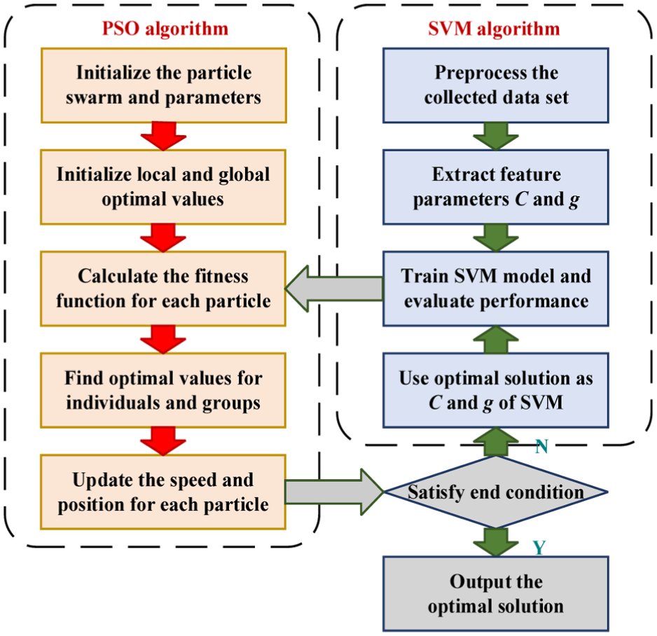
Flow chart of PSO-SVM algorithm.

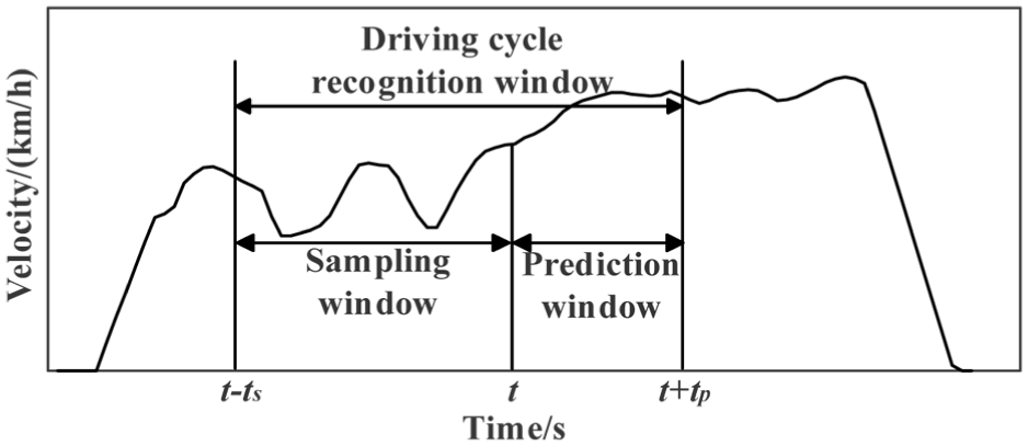
Figure 8 demonstrates the principle of the driving cycle recognition algorithm under the application of PSO-SVM. Data sampled over the past duration constitute a sampling window used to calculate characteristic parameters in real time at the current time. Based on the analysis of the sampling window, the future time t_p constitutes the prediction window, and the driving cycle category is reflected in this window. The sampling window and prediction window together constitute the process of a driving cycle recognition.⁴³ Upon completion of all driving cycle recognitions, the set of predicted cycles constitutes the final recognition result, with the entire local driving cycle being composed of three pre-defined categories.

Figure 8.

Schematic diagram of driving cycle recognition.

The optimal control strategy

As a heuristic method to solve the optimal control problem, the basic principle of ECMS is to allocate a part of the energy consumption cost to electrical energy, so that electrical energy is an equivalent substitute for fuel consumption. In the ECMS definition, instantaneous equivalent fuel consumption can be divided into actual instantaneous fuel consumption and electric equivalent fuel consumption:

{\overset{\cdot}{m}}_{eqv} (t) = {\overset{\cdot}{m}}_{fuel} (t) + {\overset{\cdot}{m}}_{elec} (t)

(10)

where ${\overset{\cdot}{m}}_{eqv} (t)$ represents the instantaneous equivalent fuel consumption; ${\overset{\cdot}{m}}_{f uel} (t)$ and ${\overset{\cdot}{m}}_{elec} (t)$ are the actual instantaneous fuel consumption and the electric equivalent fuel consumption, respectively.

Meanwhile, the equivalent factor s(t) is introduced to evaluate the average overall efficiency of the electric path under specific driving cycles. Consequently, the electrical equivalent fuel consumption can be expressed using the equation containing the equivalent factor:

{\begin{matrix} {\overset{\cdot}{m}}_{elec} (t) = \frac{s (t)}{Q_{lhv}} P_{batt} (t) p (SOC) \\ p (SOC) = 1 - {(\frac{SOC (t) - {SOC}_{ref}}{λ_{p}})}^{a} \end{matrix}

(11)

where Q_lhv is the low heating value of the fossil fuel and P_batt(t) is the battery’s power; SOC_ref is the reference value of battery SOC, and λ_p depicts the scale factor of the penalty function. In the penalty function p(SOC), the paper considers that reliable online SOC estimation can be achieved when a = 3. The reference SOC of the vehicle is obtained from the model via DP algorithm.

The equivalent fuel consumption rate under instantaneous conditions can be solved through EF in ECMS, while optimizing the instantaneous optimal output power of the engine and motor involves calculating the instantaneous power demand and constraining the power control range of the engine and motor. The constraint range is determined based on the given system state. After discretizing the upper and lower limits of the control variables into a set of discrete control variable candidates, the corresponding instantaneous fuel consumption can be calculated. Finally, the optimal control sequence under the cost function is calculated. The vehicle state and control variables can be constrained as

s . t . {\begin{matrix} SO C_{min} \leq SOC \leq SO C_{max} \\ T_{e min} \leq T_{e} \leq T_{e max} \\ T_{em \min} \leq T_{em} \leq T_{em \max} \\ ω_{e \min} \leq ω_{e} \leq ω_{e \max} \\ ω_{em \min} \leq ω_{em} \leq ω_{em \max} \end{matrix}

(12)

where $T_{e \max}$ and $T_{e \min}$ are the maximum torque and minimum torque of the engine, respectively; $ω_{e \max}$ and $ω_{e \min}$ are the maximum and minimum rotating speed of the engine, respectively; $T_{em \max}$ and $T_{em \min}$ are the maximum torque and minimum torque of the motor, respectively; $ω_{em \max}$ and $ω_{em \min}$ are the maximum and minimum rotating speed of the motor; SOC_max and SOC_min are the maximum and minimum values of the battery SOC, respectively.

Parameter optimization based on GWO

Research on HEVs typically focuses on fuel economy as the primary optimization objective. Furthermore, it is imperative to utilize real-time SOC to track the reference SOC to attain the battery depletion curve, which closely aligns with DP principle, thereby achieving optimal fuel consumption. The selection of equivalent factor (s) in ECMS will greatly influence fuel economy. An excessively large s would increase the vehicle’s electricity consumption cost, leading to a preference for using the engine and consuming fuel. Conversely, a smaller s would incline the vehicle toward using the electric motor, resulting in rapid battery depletion. In addition, considering the transmission system, the change of the transmission ratio of the main reducer f_d will also impact the vehicle’s performance. HEVs are greatly affected by external environmental factors during the driving process. A single parameter setting is insufficient to meet the requirements of different road conditions, necessitating real-time adjustments for enhanced adaptability under complex driving cycles. Therefore, the state variables and the cost function are defined as:

{\begin{matrix} x_{p} = [s, λ_{p}, f_{d}] \\ J = ω_{1} {\overset{\cdot}{m}}_{eqv} (t) + ω_{2} | {SOC}_{ref} - SOC | \end{matrix}

(13)

where x_p represents optimization variables, J is the fitness function, ω₁ and ω₂ are the weight factors. In this paper, ω₁ is 0.6, and ω₂ is 0.4. The rationale for selecting these specific weight values lies in balancing the prioritization of the multi-objective optimization.

The GWO algorithm^44–46 simulates wolf leadership and hunting methods, utilizing hierarchical alpha, beta, and delta wolves to perform prey tracking, encircling, and attacking activities. Wolves search for the best solution by gradually approaching and encircling their prey. The location of potential prey is identified by the alpha, beta, and delta wolf guidance during the hunt. The three gray wolves of the best fitness, alpha, beta, and delta, are retained to update the locations of the other search agents for each iteration, and the other wolves are under their command to hunt. The optimal result after the final iteration is the optimal value of alpha. GWO is used to optimize ECMS in three typical driving cycles, and the corresponding parameter combinations are obtained. The optimized parameter combinations are stored in a parameter library. During real-time operation, the corresponding parameters are extracted based on the driving cycle recognized by the PSO-SVM algorithm, thereby improving the vehicle’s fuel economy.

Simulation results and discussion

Local driving cycle construction result

To accurately determine the actual driving cycle of PHEBs, the paper conducts driving cycle construction on a local representative bus route through the collection, preprocessing, and synthesis of raw driving data. A vehicle tracking methodology utilizing inertial navigation systems is employed on typical local bus routes to obtain speed information. To mitigate the noise in the collected data, a Savitzky-Golay filter is applied to smooth the velocity signal, thereby aligning it more closely with the requirements of experimental processing.

Figure 9 shows the result of a local cycle after processing. In the driving cycle, the acceleration of the vehicle in the accelerating state is not less than 0.15 m/s², the acceleration of the vehicle in the decelerating state is not higher than 0.15 m/s², and the vehicle’s uniform motion maintains accelerations within the range of [−0.15,0.15] m/s². In order to be close to the real driving environment of the station, the driving cycles between the stations are regarded as kinematic segments, and the influence of a few types of kinematic segments is ignored to some extent. Parameters such as average vehicle speed, average acceleration, and velocity standard deviation in the operating conditions show errors within 5% compared to the raw data, indicating that the driving cycle can reflect the bus route’s driving characteristics, close to the real-world driving cycle.

Figure 9.

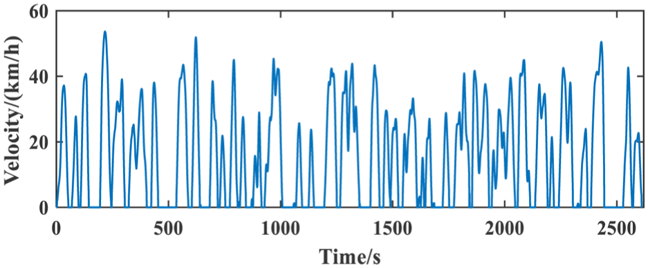
Processed local driving cycle.

Driving cycle recognition result

This study utilizes a sliding time window to extract features from all samples in the database, which comprises 11 standard bus driving cycles, and the samples are divided into 1,079 kinematic segments. The window size Δw is set to 150 s with a step Δs of 10 s. All kinematic segments are trained in PSO-SVM, 70% are used for learning and training the model, and the remaining 30% are used for data validation and testing. The training results are depicted in Figure 10. The errors of each category are within 10%, and the overall training and test accuracy reach 99.0278% and 94.7531%, respectively, which reflects the reliability of the model performance.

Figure 10.

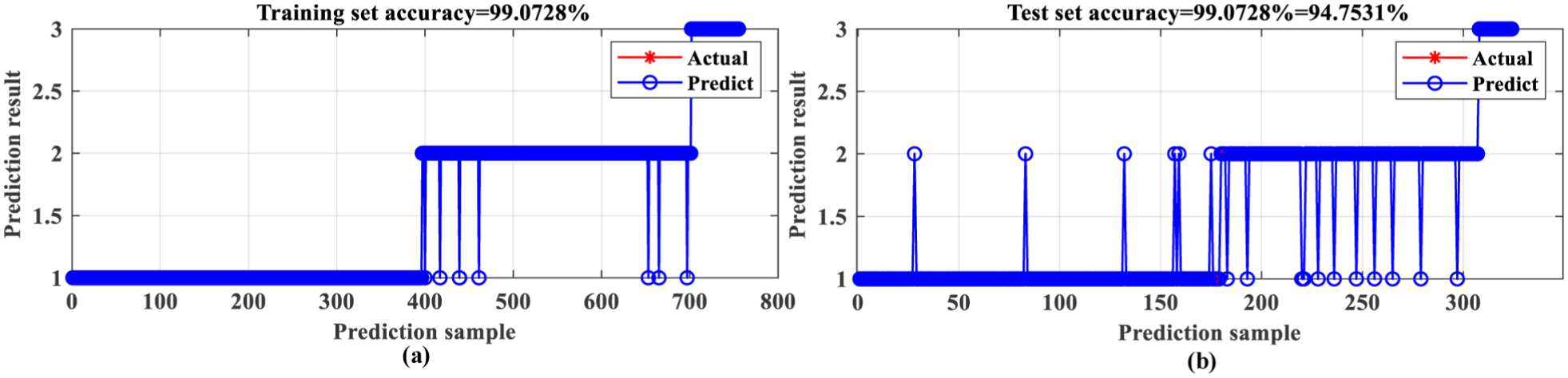
(a) Training set result; (b) classification results for the testing set.

Based on the assumption that the driving conditions will not change suddenly in a short period, the driving cycles in the future are predicted by extracting information from past driving cycles online. To ensure recognition accuracy, it is not appropriate to use too long or short recognition segments. An acceptable range is generally between 100–200 s. The historical data extraction window t_s of 150 s is selected for recognition, while the driving cycle prediction window length t_p is set at 10 s. Regarding the sensitivity of the recognition accuracy to the historical data extraction window, preliminary analyses indicated a clear trade-off. A shorter window (t_s < 100 s) makes the model overly sensitive to transient noise and reduces accuracy due to insufficient kinematic feature accumulation. Conversely, an excessively long window (t_s > 200 s) incorporates outdated driving conditions, leading to recognition lag and diminished sensitivity to actual cycle transitions. Consequently, t_s = 150 s was determined to be the optimal threshold, yielding robust accuracy. Furthermore, regarding the internal parameters of the SVM, their sensitivity was autonomously managed and optimized globally by the PSO algorithm, ensuring that the classifier avoids local optima and remains robust. A combined driving cycle is selected from the three categories in the sample database to verify the rationality of the parameter settings. Three driving cycles are CYC_MANHATTAN, CHTC_B, and CHTC_C_SUB, respectively. The recognition results, as shown in Figure 11, indicate an accuracy of 89.89% using the PSO-SVM-based method, demonstrating excellent performance.

Figure 11.

Recognition results under standard combination driving cycles.

The trained model is used to identify the local driving cycle constructed in Section III-A, and the recognition results are illustrated in Figure 12. Based on the classification and recognition results presented above, category 3 signifies suburban bus driving cycles, typically characterized by higher average and maximum speeds and relatively smaller acceleration variations. In the local driving cycle, the vehicle’s speed mostly remains below 45 km/h. However, frequent acceleration variations are observed at some traffic intersections, deviating from the requirements of category 3. Consequently, the local driving cycles predominantly exhibit urban bus cycles represented by categories 1 and 2, with only occasional instances of category 3 driving cycles occurring within the initial 500 s of the whole driving process.

Figure 12.

Recognition results under local driving cycles.

Optimization results

The paper employs MATLAB/Simulink platform to simulate the model, and the step size is set to 0.1 s to ensure the accuracy of the simulation. Based on the identified driving cycles, representative standard cycles are selected from the database to optimize key parameters. Each of the three selected cycles (CYC_MANHATTAN, CHTC_B, and CHTC_C_SUB) is repeated five times consecutively for the simulation. The final optimization results are listed in Table 5.

Table 5.

The optimization results under three representative driving cycles.

Cycle categories	s	λ _p	f _d	J
CYC_MANHATTAN	2.03	4.31	5.371	2.87
CHTC_B	1.48	2.53	5.463	4.80
CHTC_C_SUB	2.11	14.6	5.371	5.01

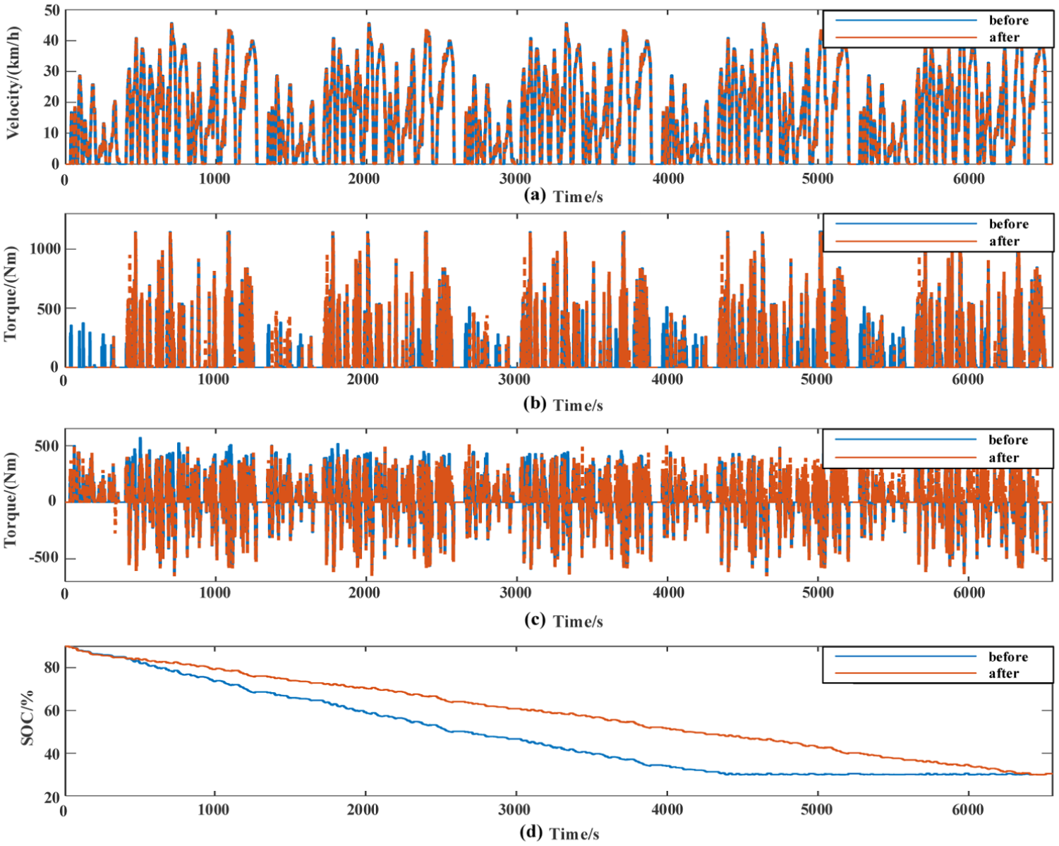
Figures 13 to 15 respectively depict schematic diagrams of vehicle performance before and after optimization under three representative driving cycles. The initial SOC of the vehicle battery is set to 90%, and each driving cycle repeats five times to ensure that the battery energy is completely depleted to the minimum value of 30%. The vehicle models employed in the three driving cycles effectively track the required vehicle speeds, demonstrating the accuracy and applicability of the models. Moreover, when battery energy is ensured to reach the minimum limit in all three driving cycles, fuel consumption is reduced by 10.6%, 11.7%, and 7.4%, respectively.

Figure 13.

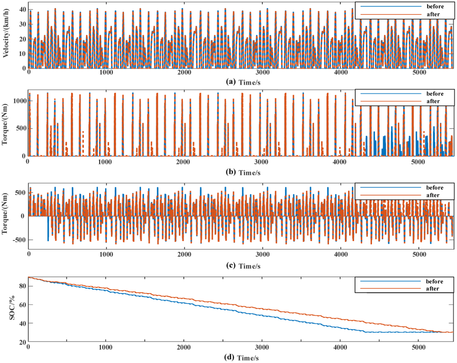
Simulation results of the CYC_MANHATTAN: (a) velocity; (b) engine; (c) motor; (d) SOC.

Figure 14.

Simulation results of the CHTC-B: (a) velocity; (b) engine; (c) motor; (d) SOC.

Figure 15.

Simulation results of the CHTC_C_SUB: (a) velocity; (b) engine; (c) motor; (d) SOC.

The paper uses the local driving cycles of five operation shifts of the PHEB to verify the effectiveness of the driving cycle recognition strategy. Based on the recognition results shown in Figure 13, the optimized key parameters corresponding to each recognized standard driving condition are updated in real-time. The speed tracking effect and torque distribution obtained are shown in Figure 16. The accurate speed tracking results verify the effectiveness of the constructed local driving cycles and demonstrate a well-optimized torque distribution.

Figure 16.

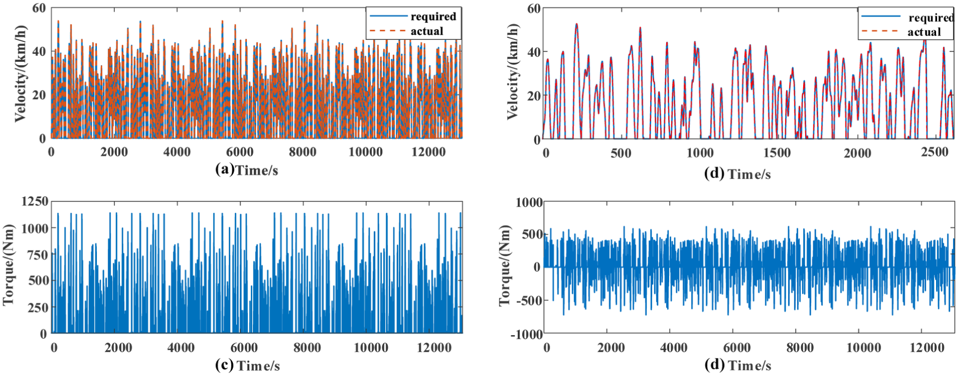
The (a) speed tracking effect; (b) details for speed tracking effect; (c) engine torque distribution under the local driving cycle; (d) motor torque distribution under the local driving cycle.

Figure 17 illustrates that in normal ECMS implementation, PHEB cannot adjust EF based on real-world driving cycles, leading to a noticeably oversized default setting of EF under the local driving cycle. The higher electrical cost of the vehicle inclines it toward fuel usage, resulting in elevated fuel consumption, while the battery capacity cannot be depleted to 30%. By contrast, although the GWO-ECMS ensures battery depletion, its charge depleting (CD) mode ends prematurely at approximately 10,800 s, at which point the vehicle enters the charge sustaining (CS) mode. In the CS mode, the PHEB is unable to further adjust engine operating efficiency and relies solely on the energy recovered through regenerative braking. Consequently, fuel consumption during this mode increases rapidly. Figure 18 shows the comparison of several strategies. Compared to the conventional ECMS, the proposed strategy reduces fuel consumption by 14.18%, achieving results that are only 3.02% higher than those of the DP algorithm. The proposed strategy adeptly tracks and closely approximates the reference SOC trajectory of DP, indicating its efficacy in meeting expected outcomes.

Figure 17.

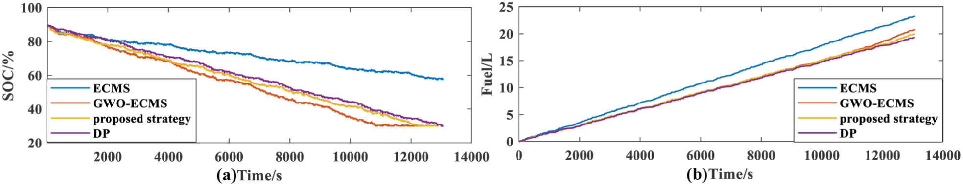
Comparison of (a) battery SOC; (b) fuel consumption under different strategies.

Figure 18.

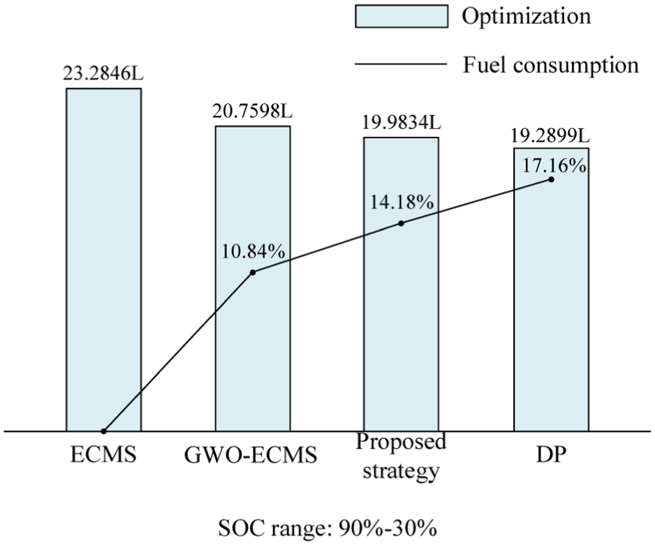
The fuel consumption with different strategies.

HIL test experiment

To ensure the reliability and accuracy of the simulation results, a hardware-in-the-loop (HIL) test is conducted to verify the proposed strategy. The schematic diagram of the HIL platform is shown in Figure 19.

Figure 19.

Diagram of the HIL simulation.

The platform is configured using VeriStand software, including the configurations of digital I/O boards, analog I/O boards, and CAN signals. The controlled object model of the hybrid electric vehicle is initially compiled by MATLAB/Simulink platform, and Dynamic Link Library (DLL) files are generated and embedded into VeriStand. The communication protocol matrix (DBC) file is written to realize the connection between the vehicle controller CAN signal and the controlled object model. The schematic diagram of the HIL test platform is shown in Figure 20.

Figure 20.

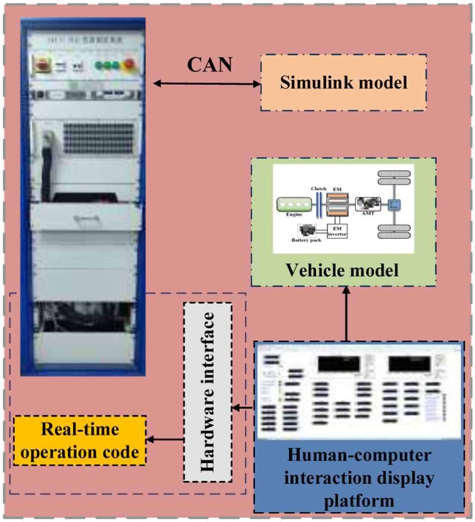
HIL test platform.

The PHEB energy management controller is the most critical part of the HIL experiment. The construction of the controller in this paper is mainly based on the MotoHawk module library developed on the Simulink platform. Firstly, the corresponding project file needs to be created according to the controller communication protocol and the model of the controller board. Secondly, the control program is written into the project file, and the controller simulation step size is preset. Finally, the project file is compiled and flashed onto the physical controller via the host PC. Through the above steps, the construction of the HIL controller can be completed.

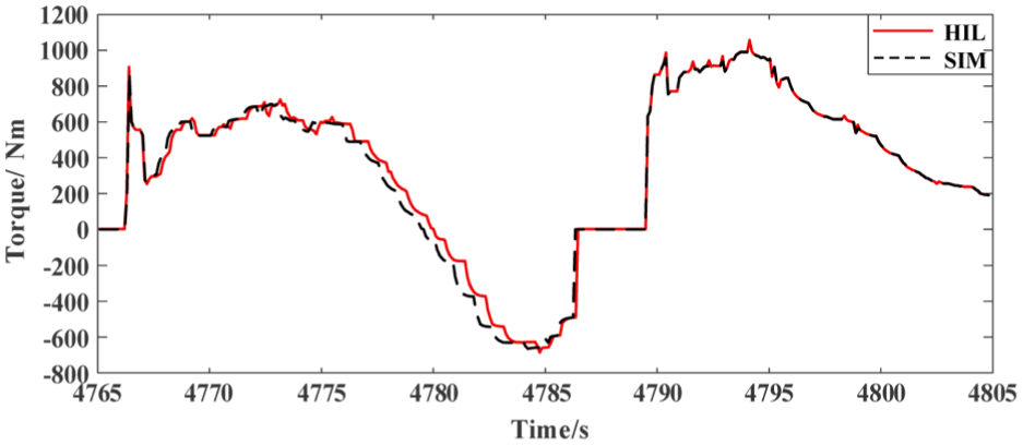
The paper selects the local driving cycle for the HIL test to verify the torque distribution. Figure 21 shows the torque distribution of both the engine and motor under the local driving cycle, from 4,765 s to 4,805 s. While the overall test results align closely with simulation tests, localized torque exhibits slight oscillations around the simulation results, indicating the difference between the physical controller and simulation.

Figure 21.

Results of the HIL test: (a) engine torque; (b) motor torque.

To improve readability and clearly demonstrate the transient differences, magnified local views of the engine and motor torque distribution during the HIL test are additionally provided in Figure 22. Furthermore, computational efficiency is a critical metric for evaluating real-time viability. During the HIL testing, the control step size of the energy management controller was configured to 10 ms. Monitoring via the host PC revealed that the average execution time for the proposed A-ECMS algorithm was approximately 5.2 ms to 6.5 ms per control cycle. Since the execution time is strictly well below the 10 ms task cycle threshold, it guarantees that no task overruns occur. This test underscores that the proposed energy management strategy can adequately meet the vehicle’s dynamic demands in real-time hardware environments.

Figure 22.

Details of total torque distribution in HIL test.

Conclusion

This paper proposed an ECMS strategy that combines driving cycle recognition and parameter optimization to improve the fuel economy of PHEB by addressing the poor adaptability of vehicles under different road conditions. To demonstrate the effectiveness of this strategy, actual data from a bus route in a local city were collected. A sample database was established based on domestic and international standard operating conditions for buses. Following feature extraction, the sample data were fed into the PSO-SVM model for training, achieving accurate driving cycle recognition. Furthermore, the optimized results of selected parameters under GWO were reflected in the three standard cycles obtained through classification. Compared to ECMS and GWO-ECMS, fuel consumption is reduced by 3.3 L and 0.78 L, respectively. Lastly, HIL test results indicated that the proposed strategy could optimize torque distribution performance.

This work still has some limitations. The accuracy of the driving cycle recognition still needs further improvement. Meanwhile, more factors can be considered as the basis for identification in the future, such as driver style and safe driving. Furthermore, as the complexity of energy management increases, managing the computational burden becomes a critical challenge. To address this, advanced optimization techniques, such as distributed optimization algorithms,⁴⁷ could be investigated in future work.

Footnotes

Handling Editor: Aarthy Esakkiappan

ORCID iD

Xiaodong Sun

Funding

The authors disclosed receipt of the following financial support for the research, authorship, and/or publication of this article: This work was supported by the “Smart Fruit” Action Plan (Guangxi Science and Technology Achievement Transformation Plan) under Project ZG2503980022.

Declaration of conflicting interests

The authors declared no potential conflicts of interest with respect to the research, authorship, and/or publication of this article.

References

Sun

Chen

Han

, et al. Adaptive real-time ECMS with equivalent factor optimization for plug-in hybrid electric buses. Energy 2024; 304: 132014.

Ali

Moulik

Söffker

. Intelligent real-time power management of multi-source HEVs based on driving state recognition and offline optimization. IEEE Trans Intell Transp Syst 2023; 24(1): 247–257.

Zhu

Yang

Wang

, et al. Energy saving performance of agricultural tractor equipped with mechanic-electronic-hydraulic powertrain system. Agriculture 2022; 12(3): 436.

Zhu

Zeng

Chen

, et al. Fuzzy adaptive energy management strategy for a hybrid agricultural tractor equipped with HMCVT. Agriculture 2022; 12(12): 1986.

Sun

Lei

, et al. Augmented continuous-control-set model predictive current control for dual three-phase PMSM drives. IEEE/ASME Trans Mechatron 2025; 30(3): 2367–2378.

Zhu

Chai

, et al. Design and performance analysis of an electric threshing drum and its speed control system for combine harvester. Biosyst Eng 2025; 260: 104313.

Sun

Lei

, et al. Adaptive model-free predictive current control for SPMSM drives with optimal virtual vector modulation. IEEE/ASME Trans Mechatron 2024; 29(4): 2569–2578.

Feng

Sun

Yang

, et al. Optimal torque sharing function control for switched reluctance motors based on active disturbance rejection controller. IEEE/ASME Trans. Mechatron 2023; 28(5): 2600–2608.

Chen

Pan

Evangelou

. Optimal energy management of series hybrid electric vehicles with engine start–stop system. IEEE Trans Contr Syst Technol 2023; 31(2): 660–675.

10.

Wang

Song

, et al. Path tracking controller and system design for agricultural tractors based on improved stanley and sliding mode algorithms considering sideslip compensation. Agronomy 2025; 15(10): 2329.

11.

Weng

Yuan

, et al. Energy optimization control of extended-range hybrid combine harvesters based on quasi-cycle power demand estimation. J Agric Eng 2025; 56(3): 1819.

12.

Zhang

Yang

Sun

, et al. A predictive PMP strategy for plug-in hybrid electric buses considering motor thermal characteristics and loss distribution. IEEE Trans Transport Electrific 2024; 10(1): 1982–1994.

13.

Zhu

Chai

, et al. Design and performance of a distributed electric drive system for a series hybrid electric combine harvester. Biosyst Eng 2023; 236: 160–174.

14.

Sun

Xue

Cai

, et al. Adaptive ECMS based on EF optimization by model predictive control for plug-in hybrid electric buses. IEEE Trans Transport Electrific 2023; 9(2): 2153–2163.

15.

Zhang

Xiao

Coskun

, et al. Comparative study of energy management in parallel hybrid electric vehicles considering battery aging. Energy 2023; 264: 123219.

16.

Sun

Jin

Xue

, et al. Adaptive ECMS with gear shift control by grey wolf optimization algorithm and neural network for plug-in hybrid electric buses. IEEE Trans Ind Electron 2024; 71(1): 667–677.

17.

Wang

. A review on the application of computer vision and machine learning in the tea industry. Front Sustain Food Syst 2023; 7: 1172543.

18.

Hsu

Liu

Chan

. A reinforcement-learning-based assisted power management with QoR provisioning for human-electric hybrid bicycle. IEEE Trans Ind Electron 2012; 59(8): 3350–3359.

19.

Weiss

Patel

Junginger

, et al. On the electrification of road transport - learning rates and price forecasts for hybrid-electric and battery-electric vehicles. Energy Policy 2012; 48: 374–393.

20.

Pang

Tang

, et al. Optimization of sprinkler irrigation scheduling scenarios for reducing irrigation energy consumption. Irrig Drain 2024; 73(4): 1329–1343.

21.

Guo

Liu

Yong

, et al. Model predictive iterative learning control for energy management of plug-in hybrid electric vehicle. IEEE Access 2019; 7: 71323–71334.

22.

Sotoudeh

HomChaudhuri

. A deep-learning-based approach to eco-driving-based energy management of hybrid electric vehicles. IEEE Trans Transport Electrific 2023; 9(3): 3742–3752.

23.

Tang

, et al. Q-learning-based supervisory control adaptability investigation for hybrid electric vehicles. IEEE Trans Intell Transp Syst 2022; 23(7): 6797–6806.

24.

Kong

Qiu

Dong

, et al. Design and development of a side spray device for UAVs to improve spray coverage in obstacle neighborhoods. Agronomy 2024; 14(9): 2002.

25.

Liu

Cai

, et al. Dual-stage feature specialization network for robust visual object detection in autonomous vehicles. Sci Rep 2025; 15(1): 15501.

26.

Shin

Sunwoo

. Vehicle speed prediction using a markov chain with speed constraints. IEEE Trans Intell Transp Syst 2019; 20(9): 3201–3211.

27.

Chen

Guo

Shen

, et al. A hierarchical energy management strategy for power-split plug-in hybrid electric vehicles considering velocity prediction. IEEE Access 2018; 6: 33261–33274.

28.

Zhang

Liu

Shen

, et al. A systematic review of modeling and control approaches for path tracking in unmanned agricultural ground vehicles. Agronomy 2025; 15(10): 2274.

29.

Sun

Ding

, et al. Path tracking control in autonomous agricultural vehicles: A systematic survey of models, methods, and challenges. Agriculture 2025; 15(23): 2522.

30.

Rabinowitz

Araghi

Gaikwad

, et al. Development and evaluation of velocity predictive optimal energy management strategies in intelligent and connected hybrid electric vehicles. Energies 2021; 14(18): 5713.

31.

Yang

, et al. Adaptive real-time optimal energy management strategy based on equivalent factors optimization for plug-in hybrid electric vehicle. Appl Energy 2017; 203: 883–896.

32.

Zhang

, et al. Adaptive equivalent consumption minimization strategy for hybrid heavy-duty truck based on driving condition recognition and parameter optimization. Energies 2020; 13(20): 5407.

33.

Feng

Han

. Progress in research on equivalent consumption minimization strategy based on different information sources for hybrid vehicles. IEEE Trans Transport Electrific 2024; 10(1): 135–149.

34.

Sun

Yao

, et al. Improved finite control set model predictive current control for permanent magnet synchronous motor with sliding mode observer. IEEE Trans Transport Electrific 2024; 10(1): 699–710.

35.

Sun

Lin

Guo

, et al. Improved deadbeat predictive current control with extended state observer for dual three-phase PMSMs. IEEE Trans Power Electron 2024; 39(6): 6769–6782.

36.

Sun

Lei

, et al. Robust predictive cascaded speed and current control for PMSM drives considering parameter variations. IEEE Trans Ind Electron 2024; 71(9): 10235–10245.

37.

Khalatbarisoltani

Han

Liu

, et al. Health-consciousness integrated thermal and energy management of connected hybrid electric vehicles using cooperative multi-agent deep reinforcement learning. IEEE Trans Intell Veh 2024. DOI: 10.1109/TIV.2024.3443448.

38.

Ericsson

. Independent driving pattern factors and their influence on fuel-use and exhaust emission factors. Transp Res Part D Transp Environ 2001; 6: 325–345.

39.

Liu

. Intelligent energy management strategy of hybrid energy storage system for electric vehicle based on driving pattern recognition. Energy 2020; 198: 117298.

40.

Bonah

Huang

, et al. Electronic nose classification and differentiation of bacterial foodborne pathogens based on support vector machine optimized with particle swarm optimization algorithm. J Food Process Eng 2019; 42(6): e13236.

41.

Ding

Yan

, et al. Classification of tea quality levels using near-infrared spectroscopy based on CLPSO-SVM. Foods 2022; 11(11): 1658.

42.

Cui

Khalatbarisoltani

Han

, et al. Driving condition-aware multi-agent integrated power and thermal management for hybrid electric vehicles. arXiv preprint arXiv:2603.27471. Epub ahead of print 29 March 2026. https://arxiv.org/abs/2603.27471.

43.

Wang

Zeng

, et al. Driving cycle recognition neural network algorithm based on the sliding time window for hybrid electric vehicles. Int J Automot Technol 2015; 16(4): 685–695.

44.

Mirjalili

Lewis

. Grey wolf optimizer. Adv Eng Softw 2014; 69: 46–61.

45.

Sunli

Jun

Hanping

, et al. Non-destructive detection for mold colonies in rice based on hyperspectra and GWO-SVR. J Sci Food Agric 2017; 98(4): 1453–1459.

46.

Sun

Tian

, et al. Nondestructive detection for moisture content in green tea based on dielectric properties and VISSA-GWO-SVR algorithm. J Food Process Preserv 2020; 44: e14421.

47.

Long

Khalatbarisoltani

. Decentralized convex optimization-based energy management strategy for modular heavy-duty fuel cell vehicles. In: Proceedings of the IEEE vehicle power and propulsion conference (VPPC), Merced, CA, USA, November 2022, pp. 1–6. IEEE.