
Abstract
Background
Postmarket device surveillance studies often have important primary objectives tied to estimating a survival function at some future time
Purpose
This article presents the details and various operating characteristics of a Bayesian adaptive design for device surveillance, as well as a method for estimating a sample size vector (determined by the maximum sample size and a preset number of interim looks) that will deliver the desired power.
Methods
We adopt a Bayesian adaptive framework, which recognizes the fact that persons enrolled in a study report their results over time, not all at once. At each interim look, we assess whether we expect to achieve our goals with only the current group or the achievement of such goals is extremely unlikely even for the maximum sample size.
Results
Our Bayesian adaptive design can outperform two nonadaptive frequentist methods currently recommended by Food and Drug Administration (FDA) guidance documents in many settings.
Limitations
Our method’s performance can be sensitive to model misspecification and changes in the trial’s enrollment rate.
Conclusions
The proposed design provides a more efficient framework for conducting postmarket surveillance of medical devices.
Introduction
Current Bayesian adaptive trial design methods have largely focused on the comparison of two or more samples, typically in the realm of hypothesis testing where the research question generally concerns whether group A differs from group B. By contrast, the one-sample problem is largely an estimation problem where the research question concerns the value of a population parameter. At the outset of a one-sample problem, a researcher sets a goal of estimating a parameter with a certain precision, sometimes with an associated acceptable threshold for efficacy. For example, we may wish to measure the percentile of medical device survival at 5 years with a 95% confidence interval (CI) having half-width no larger than .03. If the survival rate is significantly below 95%, the device may need to be recalled. Here, the precision is the half-width of the interval, which improves (shrinks) as the sample size increases, and the efficacy threshold is 95% device survival at 5 years.
The reason this is relevant in surveillance settings stems from the fact that the device should already have been established as having reasonable assurance of safety and efficacy prior to receiving market approval. After receiving approval, the relevant scientific question for the sponsor is often one of estimation (‘What is the percentile of freedom from stroke at five years post-implant for device A?’), as opposed to one of testing (‘Is the percentile of freedom from stroke at five years post-implant the same for device A and device B?’).
In such scenarios, studies may have important primary objectives tied to estimating quantities with a certain amount of precision, even if they do not necessarily have a hypothesis that is intended to be tested for the primary objective. Sample sizes in such studies should be statistically justified, even if they are not obtained through the traditional routes of power calculations performed under alternative hypotheses. The estimation approach is in agreement with 21 CFR 822, which states that a surveillance plan must include a discussion of the plan objective addressing the surveillance question(s) identified in the order; no mention of a hypothesis test approach is explicitly made in 21 CFR 822. In contrast, the current draft guidance document from the Food and Drug Administration (FDA) covering postmarket surveillance [1] calls for both study objectives and hypotheses to be included in a postmarket surveillance study plan using a standard (nonadaptive) frequentist sample size calculation. This article will elucidate the manner in which statistical sample size computation may be performed in the situation where a primary objective exists, but a hypothesis does not.
The frequentist approach can provide an estimated sample size to achieve the precision-based goal mentioned earlier under certain other constraints/assumptions (i.e., dropout rate, expected device survival percentile at the time of interest, etc.). One frequentist variant starts with the estimation of the Kaplan–Meier survival curve, applies the alternative expression for the standard error of the survival estimate by Peto et al. [2] (useful when the estimate of the survival function is close to 0 or 1), and performs an ad hoc scaling incorporating a censoring rate out to a given estimation time. The resulting expression was described in a guidance document from the FDA [3]. However, if the survival curve is assumed to arise from a Weibull distribution, then the methods described in Meeker and Nelson [4] can be applied.
This general problem of estimating a single survival curve with a certain amount of precision lends itself well to a Bayesian approach. Even under the frequentist approach to sample size estimation, we require a prior guess as to the device survival percentile at the time of interest. Instead of treating this guess as fixed, we can place a prior distribution on this parameter and then attack the problem as a Bayesian. For a general overview of Bayesian trial design, see Berry [5] as well as the most recent FDA guidance document on Bayesian methods [6]. Work summarized in Berry et al. [7] has approached similar problems of sample size in the two-sample setting by using interim looks and predictive probabilities of success. That is, one assesses the probability of achieving the given characteristics with the current sample size given the information already obtained from these observations.
Here, we too adopt a Bayesian interim look framework, which recognizes the fact that persons enrolled in a study report their results over time, not all at once. Our problem consists of predicting whether we will have enough information from the presently enrolled sample to achieve the desired characteristics after follow-up on the current group, or if given the current information, it seems futile that we will ever achieve the desired characteristics even if we continue enrollment to the prespecified maximum sample size. Simply put, at each interim look, we assess whether we expect to achieve our goals with only the current group or whether the achievement of such goals is extremely unlikely even for the maximum sample size. If either of these two situations is present, we stop enrollment at the current sample size. If not, we continue enrollment until the next interim look or the maximum sample size, whichever is dictated by the design. Once we have halted enrollment, we will continue to follow the enrolled cohort to the end of the study (e.g., 5 years minimum follow-up), at which point we evaluate the results.
Because this is a Bayesian adaptive design, each decision is based on a posterior distribution. In this design, we are making decisions at several points in time. We are deciding whether to halt enrollment at each interim sample size using a predictive calculation driven by the interim posterior, and we are making a final decision about the result of the trial based on the posterior distribution at the very end. The interim looks are set to take place when enrollment hits a prespecified number of persons. Thus, this design can be summarized as a sample size vector whose components detail the interim look sample sizes and the maximum sample size. The intent of this article is to present the general details of this design and its operating characteristics in some settings, as well as a method for estimating a sample size vector that delivers a trial with the desired power.
Methods
Before presenting our Bayesian adaptive design, we briefly review two standard frequentist designs. We continue in the device surveillance framework, where our aim is to estimate an interval for the percentile of device survival (L) at a time point of interest (T). A trial will be defined as a failure if either the precision, defined as the half-width of the interval and denoted by
Frequentist models
We compare our Bayesian results to those of two frequentist models: nonparametric Kaplan–Meier estimation and parametric Weibull estimation, both used to obtain a
Under the nonparametric Kaplan–Meier design, the researcher calculates the sample size by plugging in hypothesized parameter values and desired characteristics to an equation (shown in Appendix 1) described by an FDA guidance document [3]. Alternatively, a parametric Weibull approach discussed by Meeker and Nelson [4] can be used as a guidance, though a direct sample size calculation does not exist in this setting. Meeker and Nelson describe techniques for sample size calculation when the researcher desires an estimate of survival times at a particular percentile. However, here we are concerned with the inverse problem of estimating the survival percentile at a particular time; their methods can be adapted to this setting to a certain extent. The incongruence of the two settings arises in the desired precision: for Meeker and Nelson, the researcher specifies the acceptable degree of error for the desired percentile (e.g., if the 95th percentile is expected to be 5 years, we may willingly accept estimates between 4 and 6 years, or within 20%). In our setting, we are estimating the survival percentile
This inverse problem does not translate directly from the methods of Meeker and Nelson. Based on simulations (not shown here), the nonparametric sample size calculation appears to offer a conservative estimate for the parametric setting. When the parametric assumption is approximately correct, the estimated sample size will provide a CI with a smaller half-width relative to the nonparametric interval. Additionally, these existing frequentist methods were developed in the absence of an efficacy threshold, so no previous sample size estimation methods appear to exist for exactly the setting of our concern.
Bayesian adaptive model details
In the Bayesian setting, we no longer estimate CIs,but rather posterior credible intervals. Thus, wedetermine our Bayesian trial result using the half-width and upper limit of the posterior credible interval. Recall, we also have interim stopping rules that are assessed when enrollment has reached the interim sample size specified by the investigator: we stop enrollment for expected success when the predictive probability of success for the current sample is above a large cutoff value
During each interim look, we must evaluate the predictive distribution arising from the interim posterior, whereas for the final analysis, we evaluate the posterior distribution. For flexibility, we assume that every device has a survival time that is Weibull with a fixed shape parameter
Let
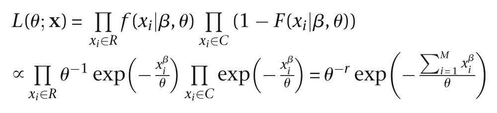
where
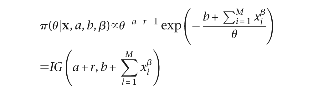
The last design element we must specify is the prior distribution on
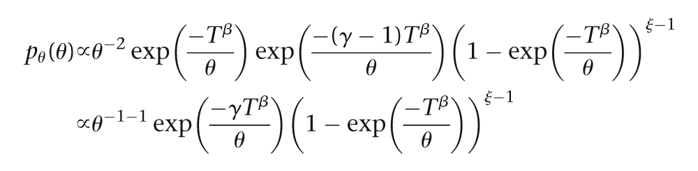
We would like a noninformative prior distribution, which for a proportion often manifests as
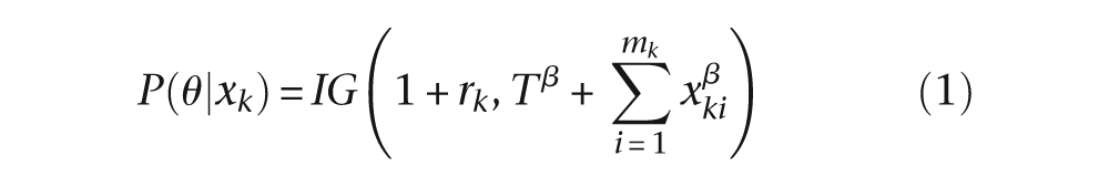
To make use of all the information available when making decisions about enrollment, we update the interim posterior when the next group is ready to enroll. So, when we check the trial at the first interim look of size
Working the other direction, since
Applying the delta method
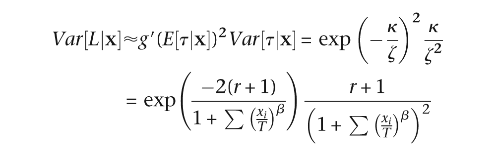
Note that
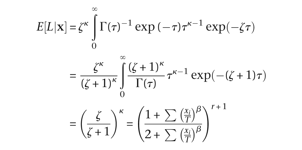
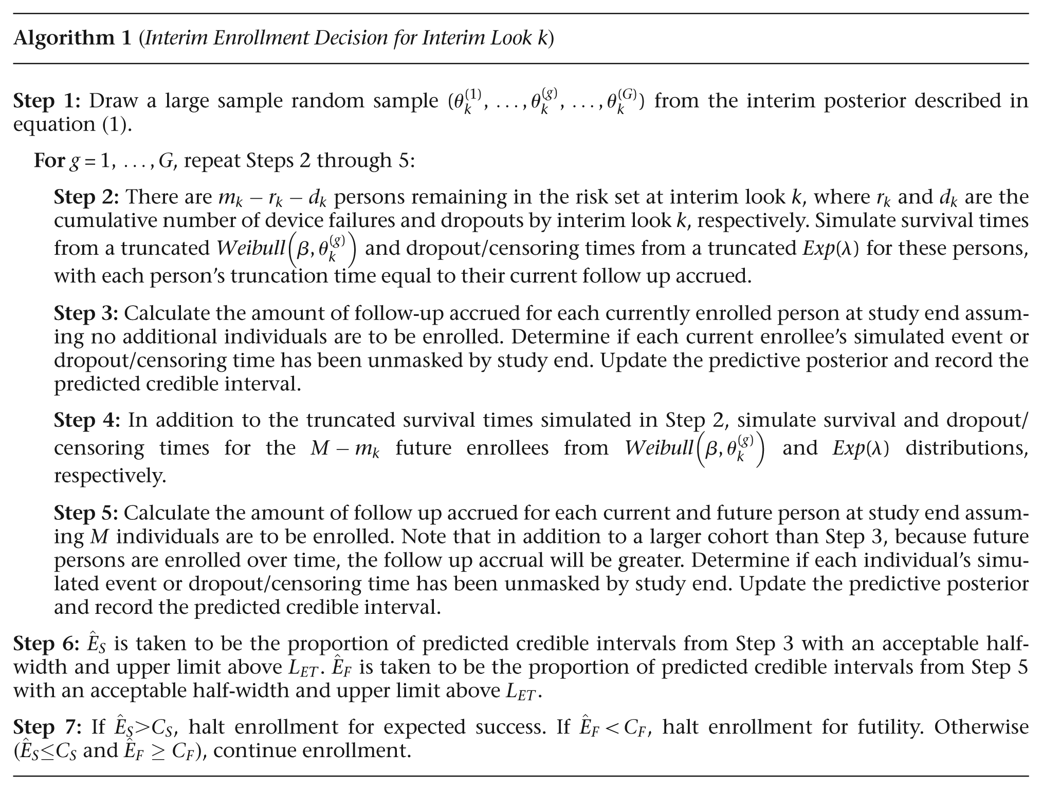
The complexity of this problem lies primarily in the computation of the expected success and futility at each interim look via Bayesian predictive probability distributions. At each interim look, we have partial information about the current group of enrollees and no information from potential future enrollees. We use the partial information at hand to update the prior to the interim posterior and then calculate the two predictive distributions. Rather than calculating the exact probabilities of expected success and futility from their corresponding predictive distributions, we estimate them using Monte Carlo sampling. First, we draw a large sample
For current enrollees, we only need to simulate remaining follow-up for those that have not yet experienced device failure nor dropped out (i.e., those remaining in the risk set at the time of the interim look) via composition from a left-truncated Weibull distribution with the sampled scale parameter
Expected success at interim look
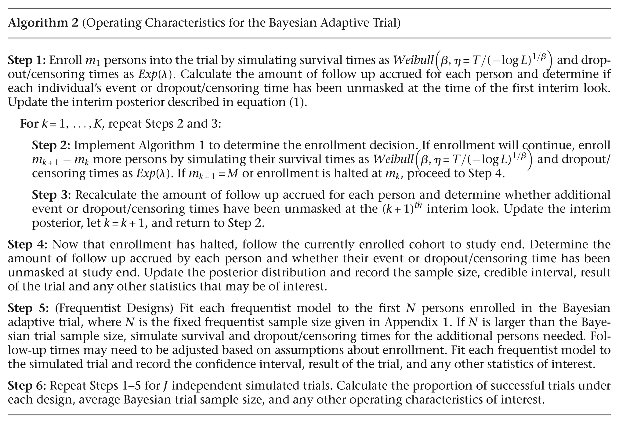
The expected success and futility calculations outlined above provide us with a one-off method of calculating
To implement this design, there are a number of parameters that need to be specified. The investigator needs to define a maximally acceptable half-width
To assess the operating characteristics of a particular design and situation, the investigator will further need to specify the true device survival percentile
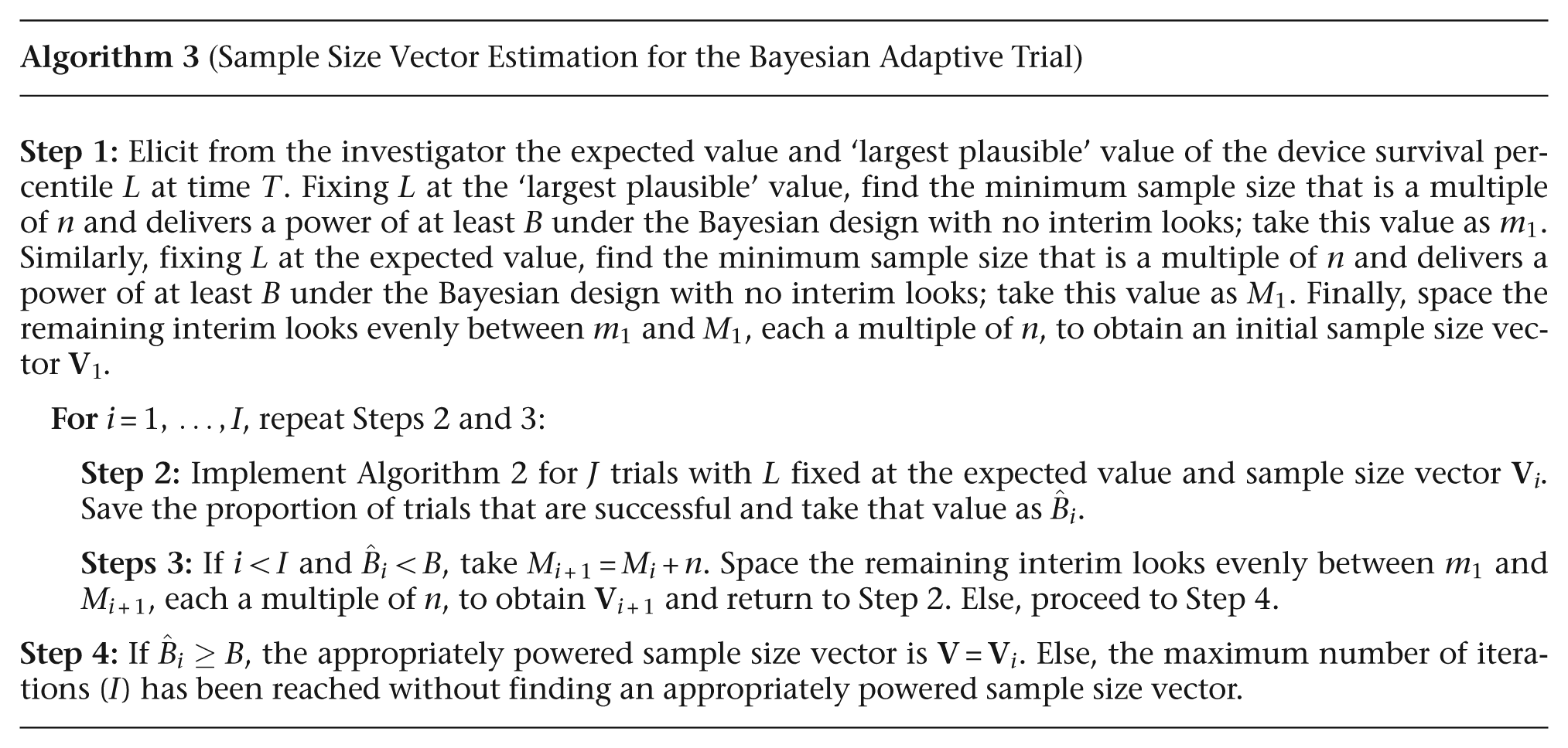
Bayesian adaptive design sample size estimation technique
To implement this Bayesian adaptive design in practice, a common question would involve the maximum sample size (M) to be used to obtain a desired power (B) for a given number of interim looks (K). Power in this setting might be the proportion of trials that will result in a sufficiently precise credible interval that contains or is completely above the efficacy threshold. This design allows for the specification of both a maximum sample size and interim sample sizes that allow for early stopping of enrollment. A sample size calculation should thus return a sample size vector,
The vector should have certain properties that motivate the sample size calculation methodology. The maximum sample size should deliver the desired power if prior expectations come to fruition. Early interim looks provide a safeguard for uncertainty about
This design provides significant flexibility regarding the placement of interim looks, but using the above principles as a guidance, we suggest the following method for determining a sample size vector that will deliver the desired power for a particular prior. Here, we simulate trials under a point-mass prior on the investigator’s expected value of
Once the investigator has provided these two hypothesized values of
With the introduction of interim looks, some of the trials will halt early and finish with a trial result that is discordant with the counterfactual trial in which enrollment had not been halted. Because we are concerned with settings in which the expected
By design,
Here, the enrollment information is again broken down into the size of each enrollment group (n) and the time lag between groups (say, 10 persons every quarter year). Given the number of trials to simulate at each iteration (J), the number of Monte Carlo samples (G) used to calculate the expected success and futility at each interim look, the cutoff values for expected success (
Results
Operating characteristics
We now report the operating characteristics of our two interim look designs with sample size vector
The dropout/censoring rate
Operating characteristics for various device survival values at 5 years (counts are out of J = 1000 trials)
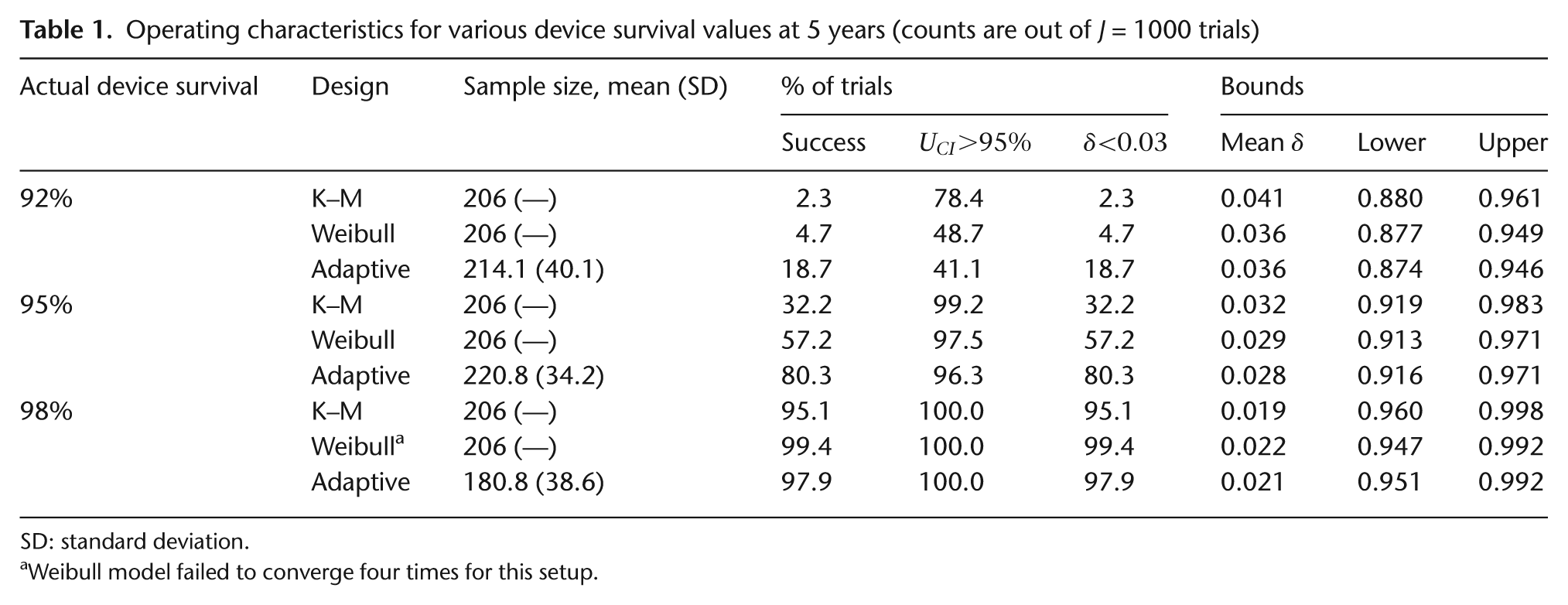
SD: standard deviation.
Weibull model failed to converge four times for this setup.
Table 1 also reports the average CI/credible interval bounds, which verify that all the models are estimating intervals centered about the actual device survival at time
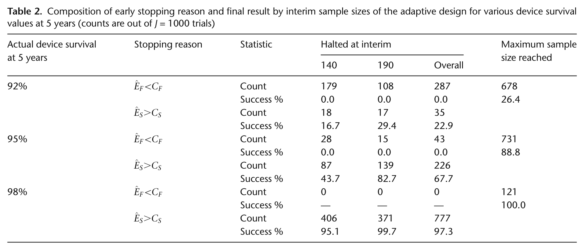
Table 2 contains a breakdown of the reasons for halting enrollment in the Bayesian adaptive trials. That is, reported are the number of times the trial was stopped for futility
Composition of early stopping reason and final result by interim sample sizes of the adaptive design for various device survival values at 5 years (counts are out of J = 1000 trials)
Next, we investigate the robustness of the three designs to shape parameter misspecification, where we expect device survival to follow
Operating characteristics of the designs in the presence of shape parameter misspecification (counts are out of J = 1000 trials)

Figure 1 shows the fitted survival curves for three
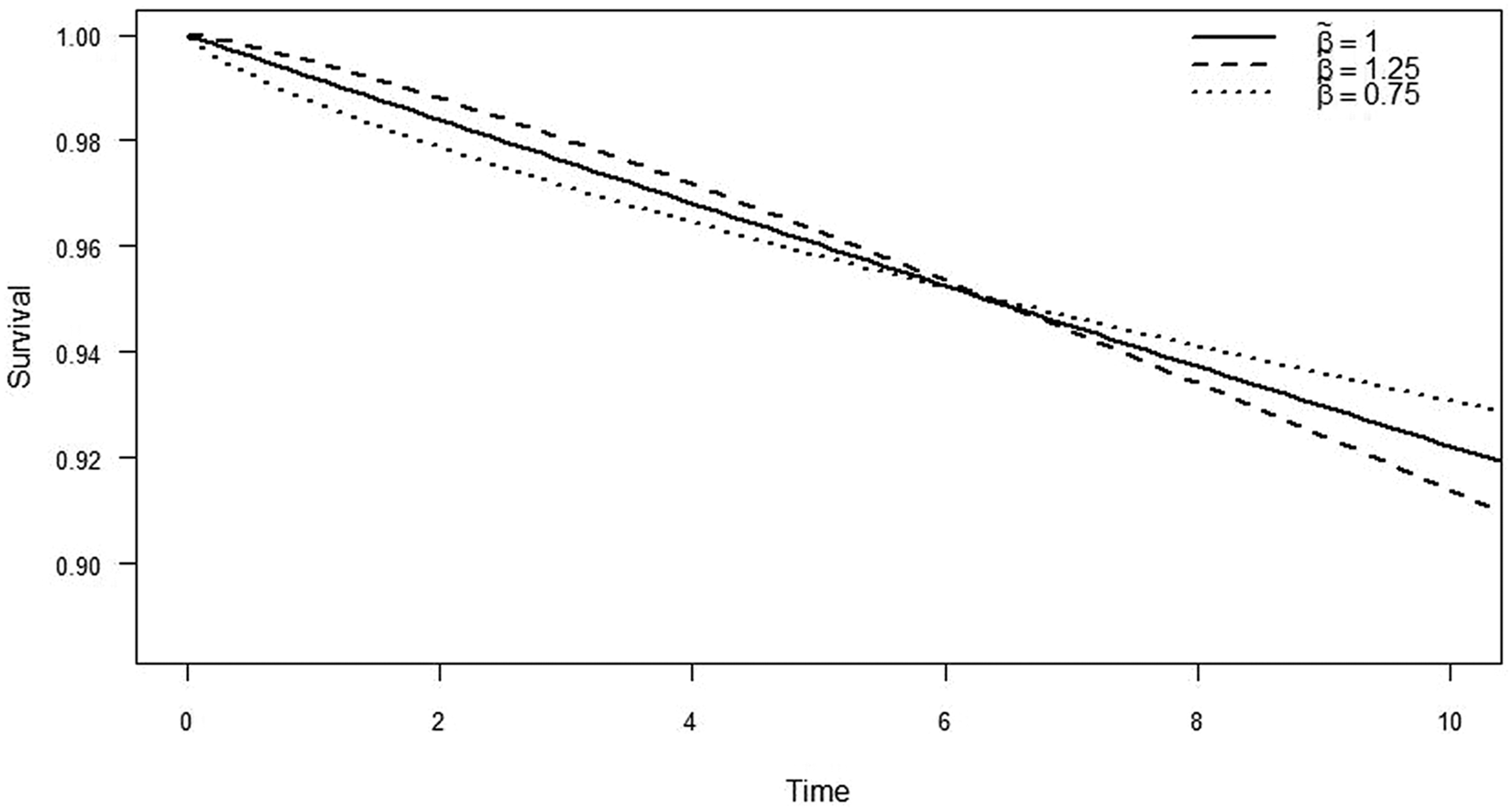
Parametric Weibull regression survival curves under shape parameter misspecification
Table 4 assesses the effect of enrollment rates. As discussed previously, the adaptive design relies on interim information to predict whether more persons should be enrolled. Faster enrollment means less information will be available at each interim look to make predictions, since information here is essentially follow-up time. The Kaplan–Meier design is again unaffected by this change as the estimate for 5-year survival is independent of anything that happens beyond 5 years. Since interim looks are driven by enrollment count and not calendar dates, the frequentist Weibull design and the Bayesian adaptive design see increased power as the enrollment rate slows, implying longer average follow-up and more information. By contrast, faster enrollment rates result in less power for these parametric designs. The Bayesian adaptive design also shows a shrinking mean sample size as enrollment rates slow. In fact, when the enrollment rate is 10 persons per half year, the Bayesian adaptive design has a similar mean sample size as both the frequentist designs and still enjoys greater power.
Operating characteristics of the designs with various enrollment rates (counts are out of J = 1000 trials)
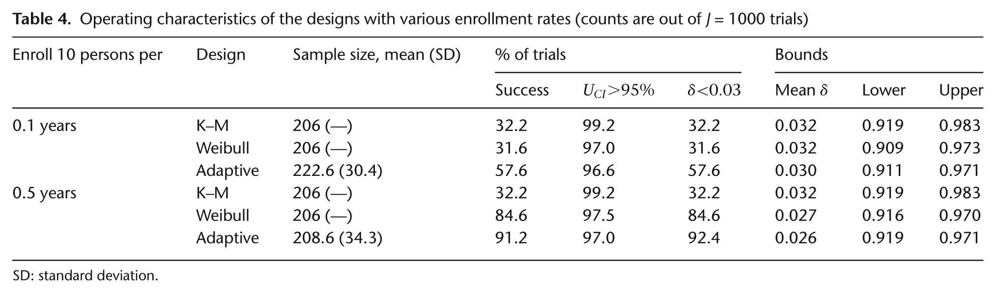
SD: standard deviation.
Sample size vector estimation
Here, we address the sample size vector estimation problem in a few different settings. Each implementation of Algorithm 3 returns a sample size vector that will deliver the desired power under the design constraints and hypothesized parameter values specified by the investigator. Recall that the primary objective is to estimate device survival at
For each sample size vector estimation in Table 5, the desired power is 80% with a dropout/censoring rate of
Estimated sample size vectors that provide 80% power
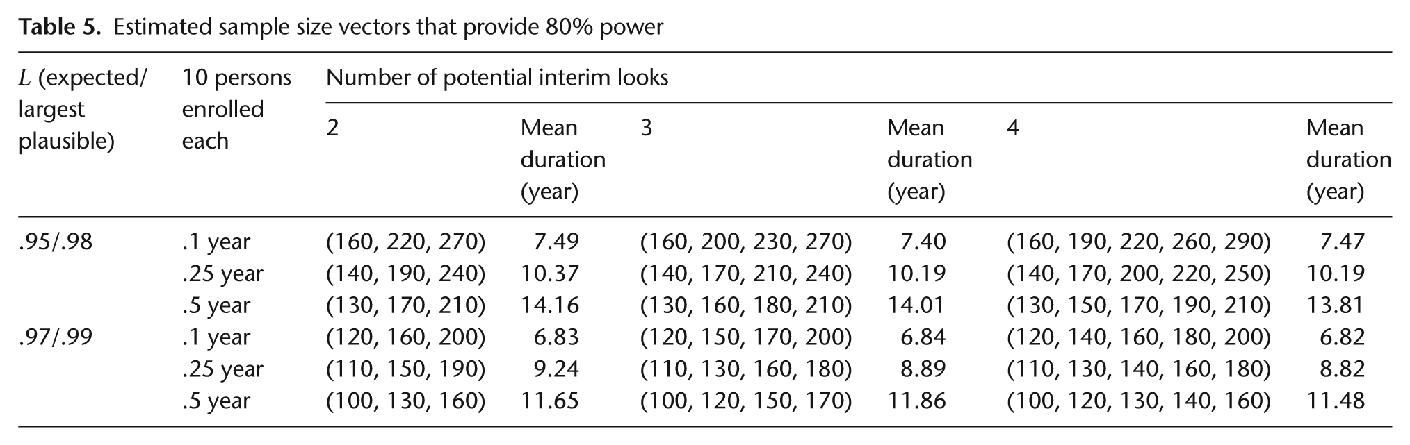
One clear pattern in Table 5 is that both slowing enrollment and greater device survival at time
Further investigation into the effect of the number of interim looks was conducted by increasing the number of trials used in each iteration of Algorithm 3 to
Discussion
The Bayesian adaptive approach provides us with a more flexible design, which results in greater power and potentially smaller mean sample sizes when actual survival at time T is different from the assumed value used to power the design. The adaptive design becomes more powerful as the enrollment rate slows and, even when our prior expectations are exactly correct, can offer a smaller average sample size while maintaining greater power. Any
The cost of adding more interim looks while maintaining the same power is the need for a larger maximum sample size. This arises because most of the halted trials do so for expected success with promising outlooks in the first enrollees. These trials with early promise regress to the true device survival rate, which occasionally results in a half-width slightly larger than
The current frequentist sample size calculation does not incorporate the idea of an efficacy threshold, whereas the Bayesian framework allows us to calculate the sample size vector for a trial that delivers the desired power in the presence of an efficacy threshold as well as a credible interval half-width requirement. Our simulations show that the frequentist sample size formula often returns a sample size with insufficient power in this setting. Admittedly, there are frequentist approaches, not discussed here, that use interim looks to reestimate sample size (see e.g., Section 6.7 in Yin [12] or Jennison and Turnbull [13]). For the Bayesian design, we have shown that a sample size vector can be reliably estimated to deliver a desired power in the presence of an efficacy threshold and a precision requirement; related applications appear in Berry et al. [7]. This provides an appropriate and detailed statistical justification for the sample sizes of device surveillance studies that are estimation driven, instead of hypothesis driven. The gains in lowered sample size and/or increased power indicate that the approach outlined here would be least burdensome for many practical scenarios.
An important limitation of both the Bayesian adaptive design and the frequentist Weibull design studied above is the fixed shape parameter. As seen in Table 3, misspecification of this parameter causes these designs to give biased results, in either a conservative or anticonservative direction. The Bayesian adaptive design shows greater robustness to misspecification than the frequentist Weibull design. Yet, in the fixed sample frequentist setting, the Weibull design can be extended to allow for simultaneous estimation of the shape and scale parameters, see Meeker and Nelson [4] or Klein and Moeschberger [8]. A corresponding Bayesian design that remains computationally feasible is a direction for future work. In our current setting, the predictive calculations can be more easily (and speedily) conducted using a one-off sampling technique. In the two-parameter nonconjugate setting, however, these draws must be made in a vastly more computationally intensive manner (e.g., by iteratively calling an MCMC sampler) since the two-parameter Weibull distribution does not admit a closed-form posterior. In principle, trial operating characteristics could still be simulated by calling BUGS or JAGS repeatedly from R using the brugs() or rjags() functions, respectively, and perhaps the multicore() function as well if using a multiple core processor. Simulating operating characteristics in this way for a nonconjugate model might take over 500 h with the current computing capacities and similar numbers of iterations used in section ‘Results’. One potential alternate solution is to use a bivariate normal approximation to the joint posterior of
Footnotes
Appendix 1
Frequentist sample size calculation for one-sample survival curve [11]:
Funding
The work of the first two authors (T.A.M. and B.P.C.) was supported by a grant from the Medtronic Corporation.
Conflict of interest
None declared.