Detecting participant noncompliance across multiple time points by modeling a longitudinal biomarker

Abstract

Introduction:

Participant noncompliance, in which participants do not follow their assigned treatment protocol, has long complicated the interpretation of randomized clinical trials. No gold standard has been identified for detecting noncompliance, but in some trials participants’ biomarkers can provide objective information that suggests exposure to non-study treatments. However, existing methods are limited to retrospectively detecting noncompliance at a single time point based on a single biomarker measurement. We propose a novel method that can leverage participants’ full biomarker history to detect noncompliance across multiple time points. Conditional on longitudinal biomarker data, our method can estimate the probability of compliance at (1) a single time point of the trial, (2) all time points, and (3) a future time point.

Methods:

Across time points, we model the biomarker as a mixture density with (latent) components corresponding to longitudinal patterns of compliance. To estimate the mixture density, we fit mixed effects models for both compliance and the biomarker. We use the mixture density to derive compliance probabilities that condition on the longitudinal biomarker data. We evaluate our compliance probabilities by simulation and apply them to a trial in which current smokers were asked to only smoke low nicotine study cigarettes (Center for the Evaluation of Nicotine in Cigarettes Project 1 Study 2). In the simulation, we investigated three different effects of compliance on the biomarker, as well as the effect of misspecification of the covariance structures. We compared probability estimators (1) and (2) to those that ignore the longitudinal correlation in the data according to area under the receiver operating characteristic curve. We evaluated estimator (3) by plotting its calibration lines. For Center for the Evaluation of Nicotine in Cigarettes Project 1 Study 2, we compared estimators (1) and (3) to a probability estimator of compliance at the last time point that ignores the longitudinal correlation.

Results:

In the simulation, for both compliance at the last time point and at all time points, conditioning on the longitudinal biomarker data uniformly raised area under the receiver operating characteristic curve across all three compliance effect scenarios. The gains in area under the receiver operating characteristic curve were smaller under misspecification. The calibration lines for the prediction of compliance closely followed 45°, though with additional variability under misspecification. For compliance at the last time point of Center for the Evaluation of Nicotine in Cigarettes Project 1 Study 2, conditioning on participants’ full biomarker history boosted area under the receiver operating characteristic curve by three percentage points. The prediction probabilities somewhat accurately approximated the non-longitudinal compliance probabilities.

Discussion:

Compared to existing methods that only use a single biomarker measurement, our method can account for the longitudinal correlation in the biomarker and compliance to more accurately identify noncompliant participants. Our method can also use participants’ biomarker history to predict compliance at a future time point.

Keywords

Clinical trials participant noncompliance detection expectation–maximization algorithm mixed effects model

Introduction

Participant noncompliance, in which participants do not follow their randomly assigned treatment protocol, has long complicated the interpretation and conduct of randomized clinical trials. Participant noncompliance often occurs when participants must self-administer the treatment without the supervision of study personnel.¹ Given this autonomy, participants may deviate from their treatment protocol for numerous reasons, including advent of side effects, insufficient benefit, and availability of commercial alternatives to the treatment.² Examples of trials with participant noncompliance include regulatory tobacco trials of very low nicotine content cigarettes, where current smokers must only smoke the study cigarettes;³ and opioid dependence trials, where patients with substance abuse disorders must self-inject study depots.^4,5 Furthermore, in longitudinal studies, multiple time points present multiple opportunities for participants to be noncompliant.

Compared to compliant participants, noncompliant participants do not receive the full dose of treatment and as such may have poor study outcomes. This may dilute the intention-to-treat (ITT) estimate.⁶ In addition, self-reported noncompliance may systematically differ from actual noncompliance according to some confounding variable.⁷ This may create a difference between the Per Protocol estimate based on self-reported compliance and the treatment effect if all participants had complied (i.e. the causal effect).⁸ As a motivating example, in the United States, the Family Smoking Prevention and Tobacco Control Act provides the Food and Drug Administration with the regulatory authority to reduce (but not eliminate) the nicotine content in commercial cigarettes if it would improve public health. Regulatory tobacco trials seek to evaluate the effect of such potential changes to commercial cigarettes. As these trials investigate interventions that could be mandated by federal law to force compliance, the causal effect is more relevant than the ITT estimator.⁹

Modeling longitudinal compliance is thus important for the following reasons. First, for completed trials, identifying compliant participants enables estimation of the causal effect,¹⁰ which may be different than both the ITT and Per Protocol estimates. Methods are thus needed to identify compliant participants to properly weigh the study outcomes and adjust for confounding, but only those for a single time point have been proposed.^11,12 Second, noncompliant participants are more likely to drop out.⁶ Methods are thus needed to identify noncompliant participants during the trial for remedial intervention.

However, in many therapeutic areas, no gold standard has been identified for detecting participant noncompliance. Trial designers must frequently rely on imperfect measures of participant noncompliance based on subjective or indirect information (e.g. self-reported compliance).^13,14 Moreover, detecting participant noncompliance falls into the broader category of diagnosis without a gold standard, a subject of considerable study. With respect to true (but unobserved) disease status, statistical methods have been able to both estimate summary measures (e.g. disease prevalence) and individually model disease progression.^15,16 Yet, few statistical methods exist for diagnosing patients whose disease status (in our case, compliance) may shift back and forth between two disease states.

In some trials, participants’ biomarkers may systematically change in response to the treatment or any alternatives to provide objective information about noncompliance. Consider three recently published regulatory tobacco trials studying the effect of very low nicotine content cigarettes (with 0.4 mg of nicotine per gram of tobacco) on smoking behavior.^3,17,18 In these trials, current smokers were randomized to smoke either normal nicotine content cigarettes (with 15.8 mg of nicotine per gram of tobacco) or very low nicotine content cigarettes provided by the study for 6 or 20 weeks. During the follow-up period, participants were asked to only smoke their assigned study cigarettes but could additionally smoke commercial cigarettes (i.e. non-study cigarettes) with normal nicotine content. Participants who smoked non-study cigarettes were considered to be noncompliant. Most participants self-reported compliance at each time point.

At each follow-up visit, participants were asked to give samples of various biomarkers including total nicotine equivalents, which measures most nicotine metabolites in the urine to evaluate recent nicotine exposure. Based on the findings of a previous study of participants who were sequestered in a hotel and only had access to very low nicotine content cigarettes, only 5% of participants randomized to very low nicotine cigarettes were expected to have total nicotine equivalents above 6.41 nmol/mL if they were fully compliant.¹⁹ However, in one trial, 63% of participants who self-reported compliance at week 6 had total nicotine equivalents above 6.41 nmol/mL.²⁰

In randomized trials of very low nicotine content cigarettes, biomarkers like total nicotine equivalents can suggest exposure to non-study cigarettes.²¹ In the absence of a gold standard for compliance, Boatman et al.¹¹ developed a method for estimating the probability of compliance at a single time point based on biomarker data collected at that time point. However, this method cannot leverage biomarker data collected at previous time points, and nor can it predict compliance at a future time point.

We propose a longitudinal method that uses biomarker data collected across multiple time points to estimate longitudinal compliance when the true compliance status is not directly observed. Specifically, we model the biomarker as a mixture density whose (latent) components correspond to different compliance patterns over time, a modeling approach similar to growth mixture models.²² Our method can estimate the probability of compliance at (1) a single time point of the trial, (2) all time points, and (3) a future time point. We first evaluate our method by simulation, examining two factors: (1) the effect of compliance on the biomarker and (2) incorrect specification of the covariance structures of the models fit. Second, we apply our method to the data collected in the Center for the Evaluation of Nicotine in Cigarettes Project 1 Study 2 (CENIC-P1S2) trial.

Methods

Overview

For our purposes, we treat the true compliance status as unobserved and binary; that is, each participant can either fully comply or not fully comply at each time point. To derive the probability of compliance at a single time point conditional on a single biomarker measurement, Boatman et al. modeled the distribution of the biomarker as a two-component mixture density of compliance and noncompliance and then used Bayes’ rule to derive the desired probability of compliance from the mixture density.¹¹ Our goal is to generalize this approach to multiple time points to identify if and when participants are noncompliant. In the longitudinal setting, the number of components in the mixture density exponentially increases beyond two as participants can shift between compliance and noncompliance at each time point. In addition, multiple observations on each participant present the possibility of correlated data. In the following section, we explain how to extend the mixture density to multiple time points while allowing for correlation among repeated measurements.

Modeling the mixture density

Let $C_{ij}$ be the true, unobserved compliance indicator (1 denotes compliance and $0$ denotes noncompliance) for the ith participant at the jth time point, where $i \in {1, \dots, n}$ and $j \in {1, \dots, K}$ . Similarly, let $B_{ij}$ be the observed biomarker of exposure for the ith participant measured at the jth time point. As participant compliance can vary over time, let $c_{k}$ be the kth compliance pattern where $k \in {1, \dots, 2^{K}}$ for $K$ time points. For example, for $K = 2$ time points, $c_{1} = {0, 0}$ , $c_{2} = {1, 0}$ , $c_{3} = {0, 1}$ , and $c_{4} = {1, 1}$ . Across time points, we specify the joint density of the biomarker as a mixture density with components corresponding to the $2^{K}$ compliance patterns. That is

\begin{matrix} f (B_{i 1}, \dots, B_{iK}) = \sum_{k = 1}^{2^{K}} P ({C_{i 1}, \dots, C_{iK}} = c_{k}) \\ f (B_{i 1}, \dots, B_{iK} | {C_{i 1}, \dots, C_{iK}} = c_{k}) \end{matrix}

(1)

A number of longitudinal models can be fit to $P ({C_{i 1}, \dots, C_{iK}} = c_{k})$ and $f (B_{i 1}, \dots, B_{iK} | {C_{i 1}, \dots, C_{iK}} = c_{k})$ . For both densities, we fit mixed effects models such that conditional on a vector of random effects, observations on the same participant are independent. For $P ({C_{i 1}, \dots, C_{iK}} = c_{k})$ , we have

\begin{matrix} P ({C_{i 1}, \dots, C_{iK}} = c_{k}) \\ = \int_{- \infty}^{\infty} P ({C_{i 1}, \dots, C_{iK}} = c_{k} | q_{i}) ψ (q_{i}) d q_{i} \\ = \int_{- \infty}^{\infty} Π_{j = 1}^{K} P (C_{ij} = c_{ij} | q_{i}) ψ (q_{i}) d q_{i} \end{matrix}

where $q_{i}$ is the participant-specific random intercept with probability density function (PDF) $ψ (q_{i})$ , and we have used the conditional independence assumption in the last equality to write $P ({C_{i 1}, \dots, C_{iK}} = c_{k} | q_{i}) = Π_{j = 1}^{K} P (C_{ij} = c_{ij} | q_{i})$ .

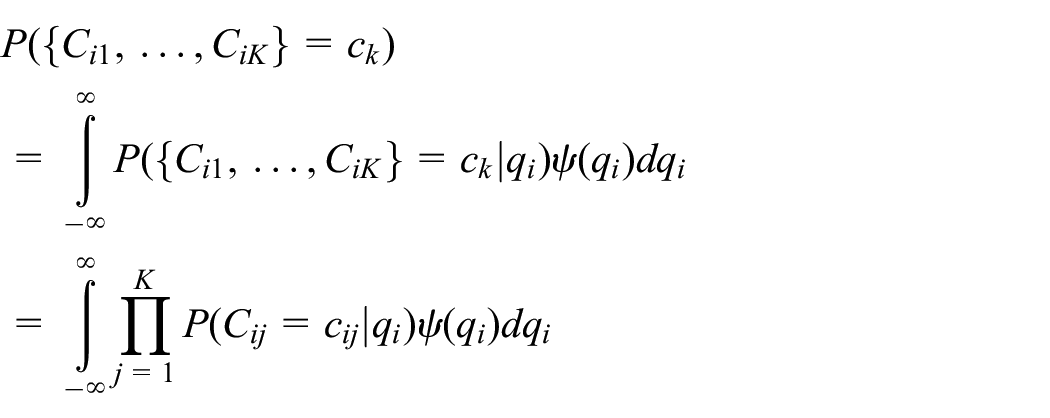
Similarly, we can use the conditional independence assumption to write $f (B_{i 1}, \dots, B_{iK} | {C_{i 1}, \dots, C_{iK}} = c_{k})$ as

\begin{matrix} f (B_{i 1}, \dots, B_{iK} | {C_{i 1}, \dots, C_{iK}} = c_{k}) \\ = \int_{- \infty}^{\infty} g (B_{i 1}, \dots, B_{iK} | {C_{i 1}, \dots, C_{iK}} = c_{k}, z_{i}) ω (z_{i}) d z_{i} \\ = \int_{- \infty}^{\infty} Π_{j = 1}^{K} g (B_{ij} | C_{ij} = c_{ij}, z_{i}) ω (z_{i}) d z_{i} \end{matrix}

where $z_{i}$ is the participant-specific random intercept with PDF $ω (z_{i})$ and is independent of compliance status.

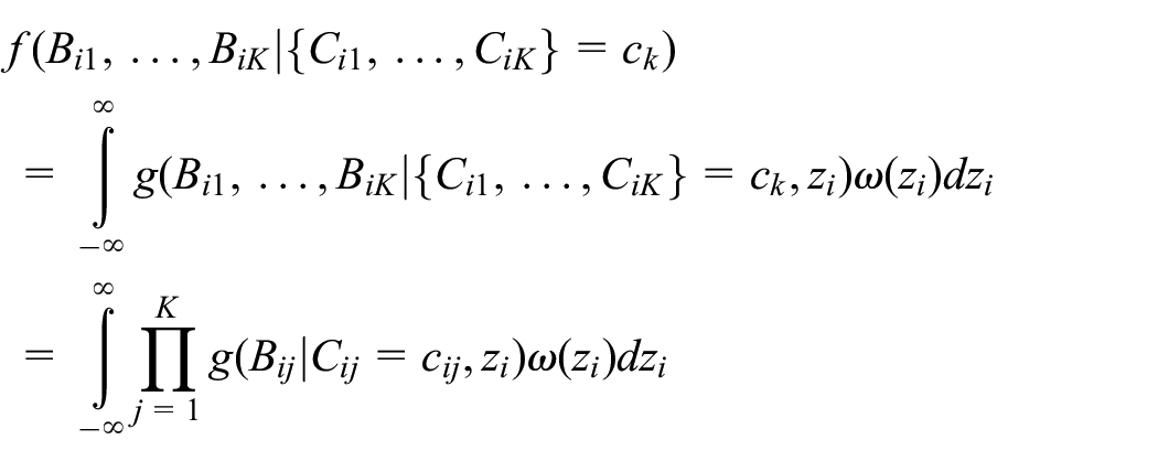
Our model setup allows us to select link functions and densities for $P (C_{ij} = c_{ij} | q_{i})$ and $g (B_{ij} | C_{ij} = c_{ij}, z_{i})$ . In addition, we can select distributions for the random intercepts $q_{i}$ and $z_{i}$ . For compliance, we assume a probit link function such that

P (C_{ij} = 1 | q_{i}) = Φ (β_{0} + q_{i})

(2)

where $Φ$ denotes the cumulative density function of the standard normal distribution and $q_{i} ~ N (0, γ^{2})$ . The inclusion of a random intercept implies a compound symmetry covariance structure. This model assumes that the probability of compliance does not change over time. For the biomarker, we assume an identity link function such that

g (B_{ij} | C_{ij} = c_{ij}, z_{i}) = N (α_{0} + α_{1} c_{ij} + z_{i}, σ^{2})

(3)

where $z_{i} ~ N (0, τ^{2})$ which again implies compound symmetry. This model assumes that the distribution of the biomarker depends only on the current compliance status.

Our method depends on properly specifying both the covariates and covariance structures for both the compliance and biomarker mixed effects models. As our method is fully likelihood-based, any number of likelihood-based tests and information criteria can be used to select which models to fit. In the application to CENIC-P1S2, we will use Bayesian information criterion (BIC) to investigate whether or not to include a fixed effect for time in the compliance mixed effects model.²³ While likelihood-based tests and information criteria can help guide model selection, the models fit may not be properly specified. Moreover, previous research of latent models has found that model misspecification of the covariance structures can lead to bias and variability in the parameter estimates.^24,25 In the simulation, we will investigate the effect of misspecifying the covariance structures on model fit.

Let $θ = (β_{0}, γ^{2}, α_{0}, α_{1}, τ^{2}, σ^{2})^{T}$ be the vector of parameters to be estimated. As is often the case with mixture densities such as equation (1), it would be difficult to directly solve for the maximum likelihood estimates of $θ$ . Instead, we can use the expectation–maximization (EM) algorithm.²⁶ Supplementary material delineates the E-step and M-step.

One advantage of this approach is that we can include participants who lack biomarker data at some time points. That is, mixed effects models estimated by maximum likelihood can inherently handle data that are missing at random. Given this assumption, estimators of $θ$ are consistent.

Deriving compliance probabilities of interest

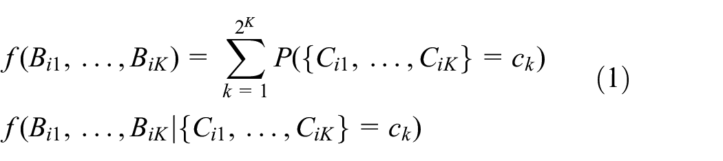
We can use the mixture density to derive compliance probabilities that condition on the longitudinal biomarker data. Intuitively, these compliance probabilities should be more accurate than methods which only condition on a single biomarker measurement. Examining all time points, we can use Bayes’ rule to derive the probability of compliance at all time points conditional on the biomarker history as

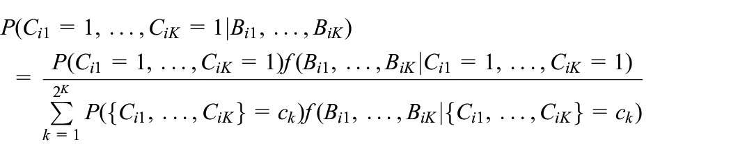
\begin{matrix} P (C_{i 1} = 1, \dots, C_{iK} = 1 | B_{i 1}, \dots, B_{iK}) \\ = \frac{P (C_{i 1} = 1, \dots, C_{iK} = 1) f (B_{i 1}, \dots, B_{iK} | C_{i 1} = 1, \dots, C_{iK} = 1)}{\sum_{k = 1}^{2^{K}} P ({C_{i 1}, \dots, C_{iK}} = c_{k}) f (B_{i 1}, \dots, B_{iK} | {C_{i 1}, \dots, C_{iK}} = c_{k})} \end{matrix}

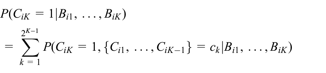
Note that both $P ({C_{i 1}, \dots, C_{iK}} = c_{k})$ and $f (B_{i 1}, \dots, B_{iK} | {C_{i 1}, \dots, C_{iK}} = c_{k})$ are already specified as part of the mixture density in equation (1) and can be estimated by plugging in the maximum likelihood estimates of $θ$ .

In addition, by summing over the relevant posterior compliance probabilities, we can derive the probability of compliance at the last time point conditional on the biomarker history as

\begin{matrix} P (C_{iK} = 1 | B_{i 1}, \dots, B_{iK}) \\ = \sum_{k = 1}^{2^{K - 1}} P (C_{iK} = 1, {C_{i 1}, \dots, C_{iK - 1}} = c_{k} | B_{i 1}, \dots, B_{iK}) \end{matrix}

Assuming that we are given biomarker data up to but not including the last time point, we can integrate out the future unobserved biomarker value to derive the prediction probability of compliance at the last time point as

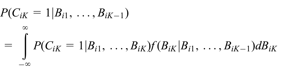
\begin{matrix} P (C_{iK} = 1 | B_{i 1}, \dots, B_{iK - 1}) \\ = \int_{- \infty}^{\infty} P (C_{iK} = 1 | B_{i 1}, \dots, B_{iK}) f (B_{iK} | B_{i 1}, \dots, B_{iK - 1}) d B_{iK} \end{matrix}

where:

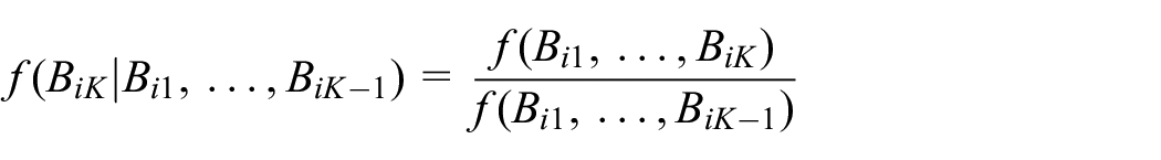
f (B_{iK} | B_{i 1}, \dots, B_{iK - 1}) = \frac{f (B_{i 1}, \dots, B_{iK})}{f (B_{i 1}, \dots, B_{iK - 1})}

Note that both the numerator and denominator of the above fraction are simply the mixture density in equation (1) given $K$ and $K - 1$ time points, respectively, and can be estimated by plugging in the maximum likelihood estimates of $θ$ for the available $K - 1$ time points.

Simulation study design

We used Monte Carlo simulation to assess the accuracy of our method in discriminating between compliers and noncompliers as well as predicting compliance at a future time point. We generated longitudinal compliance data from the mixed effects probit model outlined in equation (2), where there are no covariates and a single participant-specific random intercept. Specifically, we set $β_{0} = 0$ to make it equally likely that a participant did or did not comply with their treatment assignment at each time point on average. We set $γ^{2} = 1$ to make for equal between-subject variability and within-subject variability in compliance status.

We generated longitudinal biomarker data from the linear mixed effects model outlined in equation (3), where there is an indicator variable for compliance at the given time point and a single participant-specific random intercept. Specifically, we set the intercept of noncompliant participants to be $α_{0} = 4.0$ . Note that for the purposes of detecting noncompliance, the exact value of $α_{0}$ does not matter. We set $τ^{2} = 0.7$ and $σ^{2} = 0.3$ for two reasons: (1) to simulate more between-subject variability than within-subject variability in biomarker values conditional on compliance status with $τ^{2} > σ^{2}$ and (2) so that any compliance effect $(α_{1})$ is already standardized with $\sqrt{τ^{2} + σ^{2}} = 1$ .

To set the effect of compliance on the mean biomarker value (i.e. $α_{1}$ ), we can use the binormal receiver operating characteristic curve to solve for values of $α_{1}$ that result in a desired area under the receiver operating characteristic curve (AUC) for compliance based off a single biomarker measurement.²⁷ As the biomarkers in the CENIC trials have been found to have strong associations with compliance,²⁸ we set $α_{1} \in {- 1.5, - 1.8, - 2.1}$ which correspond to exact AUC values of ${0.856, 0.898, 0.931}$ , respectively.

To mimic the data collected in CENIC-P1S2, we set $n = 100$ participants with $K = 6$ time points. For each simulation scenario, we generated data for $1000$ trials each with no missing data. As a supplement, we ran simulations with a larger sample size to investigate a weaker compliance effect. In these simulations, $n = 500$ and $α_{1} \in {- 1.2, - 1.5, - 1.8, - 2.1}$ , where $α_{1} = - 1.2$ corresponds to an exact AUC of $0.802$ .

In addition, for both simulations of $n = 100$ and $n = 500$ , we investigated scenarios where the covariance structures of both the compliance and biomarker mixed effects models were incorrectly specified. In these scenarios, both variables were generated from first-order autoregressive (AR(1)) covariance structures but models with compound symmetry were erroneously fit. Only the regression coefficients are consistent between the data generating mechanism and the fitted models. Supplementary material provides the exact form of both covariance structures under correct and incorrect specification.

To evaluate our method, we compared the average parameter estimates to the true values, where only comparisons for $(β_{0}, α_{0}, α_{1})^{T}$ were made for the scenario of AR(1). We derived two sets of parameter estimates: (1) those for all $K = 6$ time points and (2) those for the first five time points which will be used for prediction of compliance at the last time point.

To assess the accuracy of our method in detecting noncompliance, we first compared the AUC values of the various compliance probabilities under the true parameters to the AUC values under the estimated parameters. Moreover, to protect against model overfit, AUC values were estimated from large, fixed independent test sets (i.e. we used Monte Carlo integration) as closed-form solutions are not available.

In addition, to measure the extent to which conditioning on longitudinal biomarker data improves detection of noncompliance, we compared the AUC values of $\hat{P} (C_{i 6} = 1 | B_{i 1}, \dots, B_{i 6})$ to $\hat{P} (C_{i 6} = 1 | B_{i 6})$ , where the latter conditions only on the last biomarker value. To create a comparator for $\hat{P} (C_{i 1} = 1, \dots, C_{i 6} = 1 | B_{i 1}, \dots, B_{i 6})$ , we alternatively estimated the probability of compliance at all time points as $Π_{j = 1}^{6} \hat{P} (C_{ij} = 1 | B_{ij})$ under the (erroneous) assumption that observations across time points are independent. In this expression, $\hat{P} (C_{ij} = 1 | B_{ij})$ is estimated six times corresponding to the six time points of $j$ .

To assess the accuracy of $\hat{P} (C_{i 6} = 1 | B_{i 1}, \dots, B_{i 5})$ , we plotted its calibration lines. Specifically, for each set of parameter estimates from the first five time points, we plotted the average estimated prediction probability of $\hat{P} (C_{i 6} = 1 | B_{i 1}, \dots, B_{i 5})$ against the observed probability by decile in the corresponding fixed independent test set. Code to implement our method in the programming language R is available as a GitHub repository (https://github.com/RPeterson4/Longitudinal_Noncompliance_Detection).

Application to CENIC-P1S2

We applied our method to the CENIC-P1S2 trial, which sought to evaluate the effect of very low nicotine content cigarettes with and without a nicotine patch on number of cigarettes smoked per day (NCT02301325).¹⁸ Current smokers who had no intention of quitting were randomized in a 2×2 factorial design, with very low nicotine content versus normal nicotine content cigarettes as the first factor and nicotine patch versus no nicotine patch as the second factor. During the follow-up period of 6 weeks with study visits every week, participants were asked to only smoke the study cigarettes provided by the trial but could additionally smoke commercial cigarettes.

Although previous trials of very low nicotine content cigarettes have used total nicotine equivalents as a biomarker for detecting noncompliance, nicotine patches elevate nicotine levels regardless of compliance to very low nicotine content cigarettes; therefore, we cannot use total nicotine equivalents to identify noncompliant participants in CENIC-P1S2. Instead, we used the tobacco alkaloid anatabine which has a weaker association with compliance than total nicotine equivalents.^28,29 Due to the skewness of the distribution of anatabine, and the fact that it is a concentration, we modeled it on the natural logarithm scale. In addition, some participants had observations of anatabine that fell below the limit of quantification and were thus censored. For these participants, we modified the likelihood of the conditional biomarker to accommodate left-censored observations.³⁰

A total of $n = 114$ participants from CENIC-P1S2 had anatabine data for at least one of the $K = 6$ time points. We assumed that missing anatabine data was missing at random. To improve parameter estimation for the biomarker mixed effects model, we included information from a partial gold standard of participant compliance. Specifically, we included data from the study of 23 smokers who volunteered to be sequestered in a hotel for five nights with access only to very low nicotine content cigarettes.¹⁹ We treat these anatabine data as coming from a single time point. Given that these participants were known to be compliant, their anatabine data no longer comes from a mixture density but can still be incorporated into the biomarker log likelihood. Moreover, although these anatabine data are not longitudinal, we can include them by assuming a univariate biomarker distribution of $N (μ = α_{0} + α_{1}, Σ = σ^{2} + τ^{2})$ .

In the model fit, we sought to determine whether or not compliance changed across time points. We compared the BIC of the models with a single compliance intercept versus a compliance intercept for each of the six time points. In addition, to better understand the relationship between the longitudinal anatabine values and the compliance probabilities, we constructed a spaghetti plot of log(anatabine) shaded by the probability of compliance at all time points. Similar to the simulation study, we compared $\hat{P} (C_{i 6} = 1 | B_{i 1}, \dots, B_{i 6})$ to $\hat{P} (C_{i 6} = 1 | B_{i 6})$ according to AUC. As true compliance is unknown in CENIC-P1S2, we used a model-based approach to estimate AUC. Specifically, we generated a test set based off the parameter estimates and then estimated the AUCs of both $\hat{P} (C_{i 6} = 1 | B_{i 1}, \dots, B_{i 6})$ and $\hat{P} (C_{i 6} = 1 | B_{i 6})$ . Relative to generating an independent test set as in the simulation, this approach only overestimates the AUC by approximately $0.005$ .

To assess $\hat{P} (C_{i 6} = 1 | B_{i 1}, \dots, B_{i 5})$ , we plotted the average estimated prediction probability of $\hat{P} (C_{i 6} = 1 | B_{i 1}, \dots, B_{i 5})$ against the average estimated compliance probability of $\hat{P} (C_{i 6} = 1 | B_{i 6})$ , which is known to accurately estimate compliance,²⁸ by quintile for the 97 participants with anatabine data at the last time point. Note that to estimate $P (C_{i 6} = 1 | B_{i 1}, \dots, B_{i 5})$ we used data from only the first five time points.

Results

Simulation study

For the simulation scenarios where $n = 100$ and $α_{1} \in {- 1.5, - 1.8, - 2.1}$ , Table 1 displays the bias and Monte Carlo standard deviation (MC SD) of the parameter estimates of both the compliance and biomarker mixed effects models. When the covariance structures were correctly specified, the parameters estimates were approximately unbiased across $α_{1} \in {- 1.5, - 1.8, - 2.1}$ with low MC SDs. Under incorrect specification, the biomarker coefficient parameter estimates of $(α_{0}, α_{1})^{T}$ were marginally biased, while the compliance coefficient parameter estimates of $β_{0}$ were unbiased. Both sets of parameter estimates had greater MC SDs relative to correct specification. Similar results were observed for both $K = 6$ and $K = 5$ time points. Supplementary Table 1 displays the results of the simulation scenarios where $n = 500$ and $α_{1} \in {- 1.2, - 1.5, - 1.8, - 2.1}$ .

Table 1.

Estimated bias and Monte Carlo standard deviation (MC SD) of parameter estimates for $θ$ where $n = 100$ , the number of time points $K \in {6, 5}$ , and the compliance effect $α_{1} \in {- 1.5, - 1.8, - 2.1}$ . For both compliance and the conditional biomarker, the models fit are either correctly specified with compound symmetric covariance structures, or incorrectly specified where compound symmetric covariance structures are erroneously fit to data that is generated as AR(1).

		Compliance (C_ij) parameters				Biomarker (B_ij) parameters
		Intercept		Random intercept SD		Intercept		Compliance effect		Random intercept SD		Residual SD
	Truth	$β_{0} = 0$		$γ = 1$		$α_{0} = 4.0$		$α_{1}$		$τ = 0.84$ ^a		$σ = 0.55$ ^b
		$α_{1} = - 1.5$
$K = 6$	Bias^c	$- 0.01$	$0$	$- 0.01$	−	$- 0.01$	$0.10$	$0$	$- 0.19$	$- 0.01$	−	$0$	−
	MC SD^d	$0.30$	$0.71$	$0.34$	−	$0.14$	$0.22$	$0.11$	$0.13$	$0.09$	−	$0.04$	−
$K = 5$	Bias	$0.02$	$- 0.05$	$0.04$	−	$0.01$	$0.07$	$0$	$- 0.15$	$- 0.01$	−	$0$	−
	MC SD	$0.59$	$0.90$	$0.57$	−	$0.17$	$0.23$	$0.14$	$0.17$	$0.10$	−	$0.05$	−
		$α_{1} = - 1.8$
$K = 6$	Bias	$- 0.01$	$- 0.01$	$- 0.02$	−	$- 0.01$	$0.05$	$0.01$	$- 0.11$	$- 0.01$	−	$0$	−
	MC SD	$0.19$	$0.33$	$0.18$	−	$0.12$	$0.16$	$0.08$	$0.10$	$0.08$	−	$0.03$	−
$K = 5$	Bias	$0$	$- 0.01$	$- 0.01$	−	$0$	$0.04$	$0$	$- 0.08$	$- 0.01$	−	$0$	−
	MC SD	$0.20$	$0.39$	$0.22$	−	$0.13$	$0.16$	$0.09$	$0.12$	$0.09$	−	$0.03$	−
		$α_{1} = - 2.1$
$K = 6$	Bias	$- 0.01$	$- 0.01$	$- 0.01$	−	$- 0.01$	$0.03$	$0.01$	$- 0.07$	$- 0.01$	−	$0$	−
	MC SD	$0.15$	$0.23$	$0.14$	−	$0.11$	$0.13$	$0.07$	$0.10$	$0.08$	−	$0.02$	−
$K = 5$	Bias	$0$	$- 0.01$	$- 0.01$	−	$0$	$0.02$	$0$	$- 0.04$	$- 0.01$	−	$0$	−
	MC SD	$0.16$	$0.26$	$0.17$	−	$0.12$	$0.14$	$0.08$	$0.10$	$0.08$	−	$0.03$	−

$τ^{2} = 0.7$ .

$σ^{2} = 0.3$ .

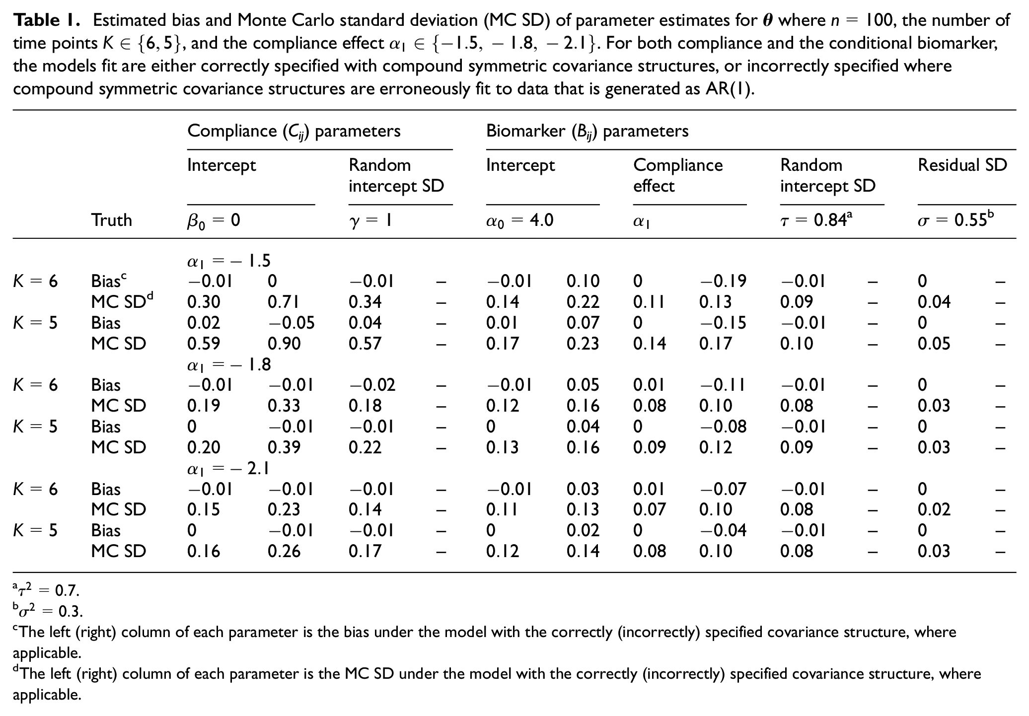
The left (right) column of each parameter is the bias under the model with the correctly (incorrectly) specified covariance structure, where applicable.

The left (right) column of each parameter is the MC SD under the model with the correctly (incorrectly) specified covariance structure, where applicable.

Across $α_{1} \in {- 1.5, - 1.8, - 2.1}$ , Table 2 displays the AUC values for both $P (C_{i 6} = 1 | B_{i 1}, \dots, B_{i 6})$ and $P (C_{i 1} = 1, \dots, C_{i 6} = 1 | B_{i 1}, \dots, B_{i 6})$ under the true parameter values and estimated parameter values. Under correct specification for both compliance probabilities, estimating the parameters resulted in a marginal loss of AUC relative to using the true values on average. Under incorrect specification, the loss of AUC was larger at about 3–5 percentage points on average.

Table 2.

True AUC values for $P (C_{i 6} = 1 | B_{i 1}, \dots, B_{i 6})$ and $P (C_{i 1} = 1, \dots, C_{i 6} = 1 | B_{i 1}, \dots, B_{i 6})$ , and average AUC values for $\hat{P} (C_{i 6} = 1 | B_{i 1}, \dots, B_{i 6})$ , $\hat{P} (C_{i 1} = 1, \dots, C_{i 6} = 1 | B_{i 1}, \dots, B_{i 6})$ , $\hat{P} (C_{i 6} = 1 | B_{i 6})$ , and $Π_{j = 1}^{6} \hat{P} (C_{ij} = 1 | B_{ij})$ , where the compliance effect $α_{1} \in {- 1.5, - 1.8, - 2.1}$ . For both compliance and the conditional biomarker, the models fit are either correctly specified with compound symmetric covariance structures, or incorrectly specified where compound symmetric covariance structures are erroneously fit to data that is generated as AR(1).

	Compliance effect $α_{1}$
	$- 1.5$	$- 1.8$	$- 2.1$
Compliance at the last time point (correctly specified)
$P (C_{i 6} = 1 \| B_{i 1}, \dots, B_{i 6})$	$0.909$	$0.950$	$0.976$
$\hat{P} (C_{i 6} = 1 \| B_{i 1}, \dots, B_{i 6})$	$0.903$	$0.948$	$0.975$
$\hat{P} (C_{i 6} = 1 \| B_{i 6})$	$0.859$	$0.901$	$0.934$
Compliance at the last time point (incorrectly specified)
$P (C_{i 6} = 1 \| B_{i 1}, \dots, B_{i 6})$	$0.891$	$0.938$	$0.969$
$\hat{P} (C_{i 6} = 1 \| B_{i 1}, \dots, B_{i 6})$	$0.859$	$0.909$	$0.944$
$\hat{P} (C_{i 6} = 1 \| B_{i 6})$	$0.855$	$0.898$	$0.931$
Compliance at all time points (correctly specified)
$P (C_{i 1} = 1, \dots, C_{i 6} = 1 \| B_{i 1}, \dots, B_{i 6})$	$0.896$	$0.943$	$0.971$
$\hat{P} (C_{i 1} = 1, \dots, C_{i 6} = 1 \| B_{i 1}, \dots, B_{i 6})$	$0.892$	$0.941$	$0.970$
$Π_{j = 1}^{6} \hat{P} (C_{ij} = 1 \| B_{ij})$	$0.784$	$0.834$	$0.880$
Compliance at all time points (incorrectly specified)
$P (C_{i 1} = 1, \dots, C_{i 6} = 1 \| B_{i 1}, \dots, B_{i 6})$	$0.906$	$0.949$	$0.974$
$\hat{P} (C_{i 1} = 1, \dots, C_{i 6} = 1 \| B_{i 1}, \dots, B_{i 6})$	$0.853$	$0.907$	$0.944$
$Π_{j = 1}^{6} \hat{P} (C_{ij} = 1 \| B_{ij})$	$0.801$	$0.852$	$0.896$

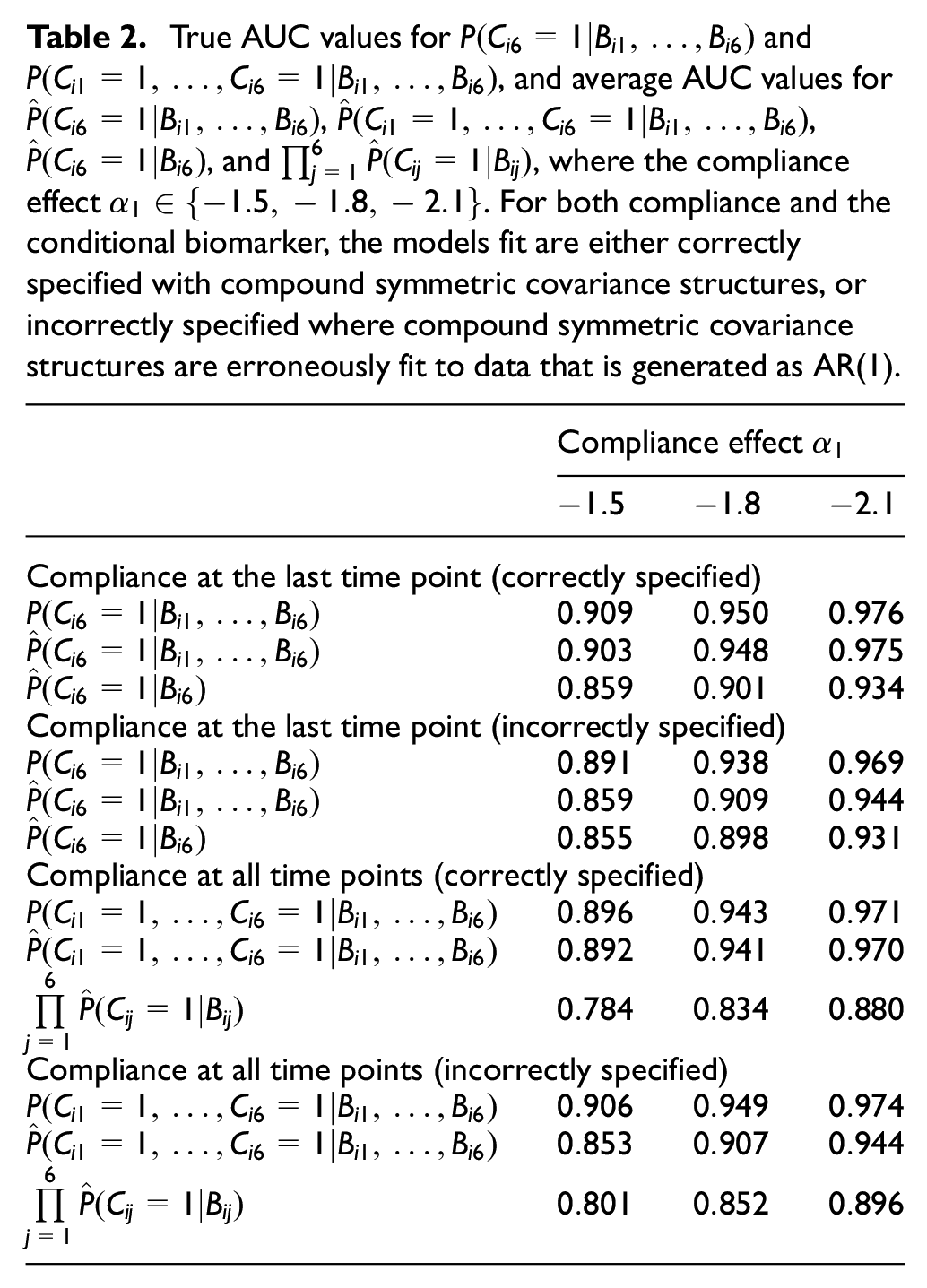
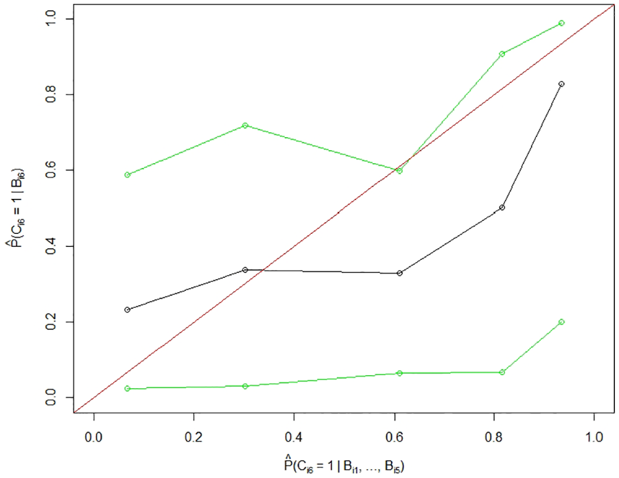
Comparing the compliance probabilities with those from Boatman et al.’s method, we found that $\hat{P} (C_{i 6} = 1 | B_{i 1}, \dots, B_{i 6})$ had uniformly higher AUC than $\hat{P} (C_{i 6} = 1 | B_{i 6})$ . The gains in AUC were moderate under correct specification and marginal under incorrect specification. Similarly, for compliance at all time points, $\hat{P} (C_{i 1} = 1, \dots, C_{i 6} = 1 | B_{i 1}, \dots, B_{i 6})$ had uniformly higher AUC than $Π_{j = 1}^{6} \hat{P} (C_{ij} = 1 | B_{ij})$ . Even with incorrect specification, the gains in AUC were about five percentage points on average (see Table 2).

For prediction of compliance at the last time point, Figure 1 displays the (gray) calibration lines of $\hat{P} (C_{i 6} = 1 | B_{i 1}, \dots, B_{i 5})$ corresponding to the sets of parameter estimates across $α_{1} \in {- 1.5, - 1.8, - 2.1}$ . The black lines mark the average calibration line and the 45° red lines mark perfect prediction. Under correct specification, the calibration lines fairly closely follow the red lines. More variability is introduced under incorrect specification. Similar to the other compliance probabilities, the AUC values of $\hat{P} (C_{i 6} = 1 | B_{i 1}, \dots, B_{i 5})$ closely approximated the true AUC values under correct specification. Under incorrect specification, there was a loss of about seven percentage points of AUC on average.

Figure 1.

Calibration lines (in gray) for $\hat{P} (C_{i 6} | B_{i 1}, \dots, B_{i 5})$ corresponding to the different sets of parameter estimates where the compliance effect $α_{1} \in {- 1.5, - 1.8, - 2.1}$ . The black lines mark the average calibration line and the 45° red lines mark perfect prediction. For both compliance and the conditional biomarker, the models fit are either correctly specified with compound symmetric covariance structures, or incorrectly specified where compound symmetric covariance structures are erroneously fit to data that is generated as AR(1).

Application to CENIC-P1S2

The model with a single compliance intercept for all time points returned a lower BIC (1882.35 vs 1902.72) compared to the model with a different compliance intercept for each time point; therefore, we assumed the more parsimonious model. Table 3 displays the parameter estimates and corresponding standard errors for $θ$ using all six time points and the first five time points for the $n = 114$ participants of CENIC-P1S2. For all six time points, compliance status was found to be highly autocorrelated with $\hat{γ} = 2.90$ . We also found that compliance had a substantial standardized effect on the biomarker with ${\hat{α}}_{1} / (\sqrt{{\hat{τ}}^{2} + {\hat{σ}}^{2}}) = - 2.36 / ({0.98}^{2} + {0.72}^{2}) = - 1.94$ . The conditional biomarker was fairly autocorrelated with $\hat{τ} = 0.98$ .

Table 3.

Parameter estimates and standard errors (SE) for θ using all six time points (n = 114) and the first five time points (n = 114) of CENIC-P1S2 for participants who had at least one anatabine value.

	Compliance (C_ij) parameters				Biomarker (B_ij) parameters
	Intercept		Random intercept SD		Intercept		Compliance effect		Random intercept SD		Residual
	${\hat{β}}_{0}$	SE $({\hat{β}}_{0})$	$\hat{γ}$	SE $(\hat{γ})$	${\hat{α}}_{0}$	SE $({\hat{α}}_{0})$	${\hat{α}}_{1}$	SE $({\hat{α}}_{1})$	$\hat{τ}$	SE $(\hat{τ})$	$\hat{σ}$	SE $(\hat{τ})$
$K = 6$	$- 0.36$	$0.83$	$2.90$	$0.81$	$- 3.56$	$0.27$	$- 2.36$	$0.15$	$0.98$	$0.14$	$0.72$	$0.04$
$K = 5$	$0.15$	$0.86$	$3.54$	$1.18$	$- 3.42$	$0.25$	$- 2.34$	$0.17$	$0.88$	$0.13$	$0.70$	$0.05$

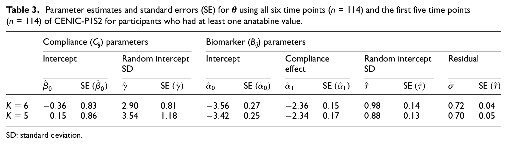
SD: standard deviation.

Figure 2 displays the spaghetti plot of log(anatabine) for the time points when participants had data for CENIC-P1S2. For the anatabine values, we find that consistency is as important as magnitude in determining the probabilities of compliance at all time points. Our method assigned high probabilities to participants who always had relatively low anatabine values. Conversely, our method assigned low probabilities to participants who had low anatabine values at some time points but upticks at others.

Figure 2.

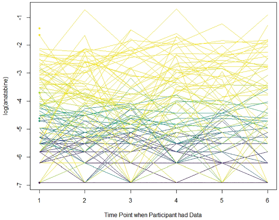
Spaghetti plot of the longitudinal biomarker for the time points when participants had data for CENIC-P1S2. Lines are shaded by the probability of compliance at all time points. Lighter lines indicate a probability closer to 0 while darker lines indicate a probability closer to 1. The x-axis refers to the time points when participants had data. For example, a participant with data only at time points 1 and 4 would have a line from 1 to 2.

For compliance at the last time point, the AUC of $\hat{P} (C_{i 6} = 1 | B_{i 1}, \dots, B_{i 6})$ was $0.943$ while the AUC of $\hat{P} (C_{i 6} = 1 | B_{i 6})$ was $0.916$ , a gain of $0.027$ AUC. For prediction of compliance at the last time point, Figure 3 compares $\hat{P} (C_{i 6} = 1 | B_{i 1}, \dots, B_{i 5})$ to $\hat{P} (C_{i 6} = 1 | B_{i 6})$ . The green lines mark the bounds of the 95% prediction interval and the 45° red line marks perfect prediction. The line of quintiles fairly follows the red line, indicating that the probabilities of $\hat{P} (C_{i 6} = 1 | B_{i 1}, \dots, B_{i 5})$ somewhat accurately approximate the probabilities of $\hat{P} (C_{i 6} = 1 | B_{i 6})$ .

Figure 3.

Averaged estimated prediction probability of $\hat{P} (C_{i 6} = 1 | B_{i 1}, \dots, B_{i 5})$ plotted against the average estimated compliance probability of $\hat{P} (C_{i 6} = 1 | B_{i 6})$ by quintile for the 97 participants of CENIC-P1S2 who had anatabine data at the last time point. The 45° red line marks perfect prediction and the green lines mark the bounds of the 95% prediction interval.

Discussion

For trials in which there is no known gold standard for measuring compliance, we have developed a method that can use longitudinal biomarker data to more accurately identify compliant participants, as well as predict which participants may or may not comply in the future. Our simulation study confirms that our method, which conditions on participants’ full biomarker history, is better able to discriminate between compliers and noncompliers compared to Boatman et al.’s method which conditions only on the most recent biomarker value. We also find that our prediction of compliance at a future time point conditional on biomarker data from previous time points is well-calibrated. Furthermore, when the covariance structures of both models for compliance and the biomarker are misspecified, we find that our method still has high discrimination. These results held across a range of differences in the biomarker between compliant and noncompliant participants.

In the application to the biomarker data collected from the $n = 114$ participants of CENIC-P1S2, we showed that our method was able to improve upon Boatman et al.’s method in estimating compliance at the last time point. In addition, the prediction probability was able to somewhat accurately predict compliance at the last time point. Although we only investigated a subset of compliance patterns in this article, our method can be used to estimate the compliance probability for any compliance pattern given observed biomarker data.

As demonstrated with the inclusion of the non-longitudinal hotel dataset, our method can include information from a partial gold standard. When compliance is known at all time points for a subset of participants, both longitudinal and non-longitudinal biomarker data can be incorporated into the biomarker log likelihood with the corresponding observed compliance patterns. Moreover, it is straightforward to adapt our method when compliance is known at some time points for a subset of participants. As only a subset of compliance patterns would be plausible, a mixture density with fewer compliance patterns can be fit for these participants.

For completed trials, our method can be used to improve estimation of causal effects. For example, the probability of compliance at all time points can be used to modify an inverse probability of compliance weight to more accurately weight the study outcomes, similar to Boatman et al.¹¹ For trials in progress, the prediction probability can be used to identify noncompliant participants to enable remedial intervention. This could both improve study outcomes and reduce the number of dropouts, the latter of which may also reduce the sample size at the end of the trial. That is, with fewer dropouts, fewer additional participants may be needed to maintain statistical power.

Although our method belongs to the broader class of growth mixture models commonly found in the psychometrics literature,³¹ there are some key differences that distinguish our method. Specifically, the number of latent groups we considered (2⁶ = 64) is substantially greater than in more traditional applications where 2–4 latent groups are more common. When the number of latent groups is small, the (marginal) probability of group membership is generally treated as a free parameter and the longitudinal data trajectory within each group is generally unconstrained. Given the large number of latent groups in our study, however, we constrained the probabilities of the latent groups by assuming mixed effects models for both compliance and the biomarker. Under this relatively simple modeling structure, the number of parameters is kept small relative to the number of latent groups.

Although we considered relatively straightforward models for both compliance and the biomarker, our method can be extended to fit richer longitudinal models with more parameters. Our method can also be adapted to a measure of compliance consisting of more than two levels, but substantially more computational power would be required to fit the models. That is, with more levels of compliance the number of compliance patterns would exponentially increase.

Our method does have some limitations. First, although mixed effects models can handle data which are missing at random, this assumption may not be realistic when studying compliance. Second, we have defined compliance to be a discrete random variable. Adapting our method to a continuous measure of compliance is not straightforward. Third, the compliance effect on the biomarker must be substantial to be reliably detected and larger samples are required to detect smaller compliance effects. Fourth, although likelihood-based tests and information criteria can help identify the optimal model structure, we have not developed model diagnostics specific to our method. Fifth, fitting mixed effects models to both observed and unobserved variables is computationally intensive and parameter estimates may be sensitive to initial starting values. Finally, as compliance is unobserved, it remains difficult to evaluate the discriminative performance of our method for clinical trials in practice. Model-based approaches can be used as in the applied example to CENIC-P1S2, but the AUC will likely be marginally overestimated.

In future clinical trials where a biomarker is known to respond to deviations from the treatment assignment, our method can be used to identify noncompliant participants both during and after the trial. The mode of noncompliance is immaterial; provided that noncompliance has a systematic effect on the biomarker, our method can be used for both participants who do not take any treatments and those who take alternatives. With this novel statistical method, trial designers should be better able to both adjust for noncompliance and prevent it from happening.

Supplemental Material

Compliance_Paper_Clean_3rd_Submission_Supp – Supplemental material for Detecting participant noncompliance across multiple time points by modeling a longitudinal biomarker

Supplemental material, Compliance_Paper_Clean_3rd_Submission_Supp for Detecting participant noncompliance across multiple time points by modeling a longitudinal biomarker by Ross L Peterson, Joseph S Koopmeiners, Tracy T Smith, Sharon E Murphy, Eric C Donny and David M Vock in Clinical Trials

Footnotes

Declaration of conflicting interests

The author(s) declared no potential conflicts of interest with respect to the research, authorship, and/or publication of this article.

Funding

The author(s) disclosed receipt of the following financial support for the research, authorship, and/or publication of this article: This study was funded by the National Heart, Lung, and Blood Institute (award number T32HL129956), the National Cancer Institute (award numbers R01CA214825 and R01CA225190), the National Institute on Drug Abuse (award numbers R01DA046320, R03DA041870, and U54-DA031659) and National Center for Advancing Translational Science (award number UL1TR002494). The content is solely the responsibility of the authors and does not necessarily represent the official views of the National Institutes of Health or Food and Drug Administration.

ORCID iD

Ross L Peterson

Supplemental material

Supplemental material for this article is available online.

References

Stephenson

Rowe

Haynes

, et al. Is this patient taking the treatment as prescribed? JAMA 1993; 269(21): 2779–2781.

Boza

Milanes

Slater

, et al. Patient noncompliance and overcompliance behavior patterns underlying a patient’s failure to ’follow doctor’s orders.’Postgrad Med 1987; 81(4): 163–170.

Donny

Denlinger

Tidey

, et al. Randomized trial of reduced-nicotine standards for cigarettes. New Engl J Med 2015; 373(14): 1340–1349.

Center for Drug Evaluation Research. Joint meeting of psychopharmacologic drugs advisory committee and the drug safety and risk management advisory committee. Technical report, Food and Drug Administration, 2017, https://www.federalregister.gov/documents/2020/08/28/2020-18951/joint-meeting-of-the-psychopharmacologic-drugs-advisory-committee-and-the-drug-safety-and-risk

Center for Drug Evaluation Research. Joint meeting of anesthetic and analgesic drug products advisory committee and drug safety and risk management advisory committee. Technical report, Food and Drug Administration, 2018, https://www.fda.gov/media/99493

van Dulmen

Sluijs

Van Dijk

, et al. Patient adherence to medical treatment: a review of reviews. BMC Health Serv Res 2007; 7(1): 55.

Jin

Sklar

Min Sen Oh

, et al. Factors affecting therapeutic compliance: a review from the patient’s perspective. Ther Clin Risk Manag 2008; 4(1): 269–286.

Bellamy

Lin

Ten Have

TR.

An introduction to causal modeling in clinical trials. Clin Trials 2007; 4(1): 58–73.

Koopmeiners

Vock

Boatman

, et al. The importance of estimating causal effects for evaluating a nicotine standard for cigarettes. Nicotine Tobacco Res 2019; 21(Suppl. 1): S22–S25.

10.

Rosenbaum

Rubin

DB.

The central role of the propensity score in observational studies for causal effects. Biometrika 1983; 70(1): 41–55.

11.

Boatman

Vock

Koopmeiners

, et al. Estimating causal effects from a randomized clinical trial when noncompliance is measured with error. Biostatistics 2017; 19(1): 103–118.

12.

Boatman

Vock

Koopmeiners

JS.

Efficiency and robustness of causal effect estimators when noncompliance is measured with error. Stat Med 2018; 37(28): 4126–4141.

13.

Farmer

KC.

Methods for measuring and monitoring medication regimen adherence in clinical trials and clinical practice. Clin Ther 1999; 21(6): 1074–1090

14.

DiMatteo

MR.

Variations in patients’ adherence to medical recommendations: a quantitative review of 50 years of research. Med Care 2004; 42(3): 200–209.

15.

Joseph

Gyorkos

Coupal

Bayesian estimation of disease prevalence and the parameters of diagnostic tests in the absence of a gold standard. Am J Epidemiol 1995; 141(3): 263–272.

16.

Cook

Lawless

JF.

Multistate models for the analysis of life history data. Boca Raton, FL: CRC Press, 2018.

17.

Hatsukami

Luo

Jensen

, et al. Effect of immediate vs gradual reduction in nicotine content of cigarettes on biomarkers of smoke exposure: a randomized clinical trial. JAMA 2018; 320(9): 880–891.

18.

Smith

Koopmeiners

Tessier

, et al. Randomized trial of low-nicotine cigarettes and transdermal nicotine. Am J Prev Med 2019; 57(4): 515–524.

19.

Denlinger

Smith

Murphy

, et al. Nicotine and anatabine exposure from very low nicotine content cigarettes. Tob Regul Sci 2016; 2(2): 186–203.

20.

Nardone

Donny

Hatsukami

, et al. Estimations and predictors of non-compliance in switchers to reduced nicotine content cigarettes. Addiction 2016; 111(12): 2208–2216.

21.

Benowitz

Nardone

Hatsukami

, et al. Biochemical estimation of noncompliance with smoking of very low nicotine content cigarettes. Cancer Epidemiol Biomarkers Prev 2015; 24(2): 331–335.

22.

Duncan

Strycker

LA.

An introduction to latent variable growth curve modeling: concepts, issues, and application. New York: Routledge, 2013.

23.

Schwarz

Estimating the dimension of a model. Ann Stat 1978; 6(2): 461–464.

24.

Pepe

Alonzo

Reply to letter to editor. Stat Med 2001; 20: 656–660.

25.

Albert

Dodd

LE.

A cautionary note on the robustness of latent class models for estimating diagnostic error without a gold standard. Biometrics 2004; 60(2): 427–435.

26.

Dempster

Laird

Rubin

DB.

Maximum likelihood from incomplete data via the EM algorithm. J Royal Stat Soc: Series B 1977; 39(1): 1–22.

27.

Pepe

. The receiver operating characteristic curve. In: Pepe

(ed.) The statistical evaluation of medical tests for classification and prediction. Oxford: Oxford University Press, 2003, pp. 66–85.

28.

Boatman

Casty

Vock

, et al. Classification accuracy of biomarkers of compliance. Tobacco Regulat Sci 2019; 5(3): 301–319.

29.

VonWeymarn

Thomson

Donny

, et al. Quantitation of the minor tobacco alkaloids nornicotine, anatabine, and anabasine in smokers’ urine by high throughput liquid chromatography–mass spectrometry. Chem Res Toxicol 2016; 29(3): 390–397.

30.

Vock

Davidian

Tsiatis

, et al. Mixed model analysis of censored longitudinal data with flexible random-effects density. Biostatistics 2011; 13(1): 61–73.

31.

Coulacoglou

Saklofske

DH.

Psychometrics and psychological assessment: principles and applications. Cambridge, MA: Academic Press, 2017.

Supplementary Material

Please find the following supplemental material available below.

For Open Access articles published under a Creative Commons License, all supplemental material carries the same license as the article it is associated with.

For non-Open Access articles published, all supplemental material carries a non-exclusive license, and permission requests for re-use of supplemental material or any part of supplemental material shall be sent directly to the copyright owner as specified in the copyright notice associated with the article.

0.00 MB

0.19 MB