Meta-analysis of rare adverse events in randomized clinical trials: Bayesian and frequentist methods

Abstract

Background/aims:

Regulatory approval of a drug or device involves an assessment of not only the benefits but also the risks of adverse events associated with the therapeutic agent. Although randomized controlled trials (RCTs) are the gold standard for evaluating effectiveness, the number of treated patients in a single RCT may not be enough to detect a rare but serious side effect of the treatment. Meta-analysis plays an important role in the evaluation of the safety of medical products and has advantage over analyzing a single RCT when estimating the rate of adverse events.

Methods:

In this article, we compare 15 widely used meta-analysis models under both Bayesian and frequentist frameworks when outcomes are extremely infrequent or rare. We present extensive simulation study results and then apply these methods to a real meta-analysis that considers RCTs investigating the effect of rosiglitazone on the risks of myocardial infarction and of death from cardiovascular causes.

Results:

Our simulation studies suggest that the beta hyperprior method modeling treatment group-specific parameters and accounting for heterogeneity performs the best. Most models ignoring between-study heterogeneity give poor coverage probability when such heterogeneity exists. In the data analysis, different methods provide a wide range of log odds ratio estimates between rosiglitazone and control treatments with a mixed conclusion on their statistical significance based on 95% confidence (or credible) intervals.

Conclusion:

In the rare event setting, treatment effect estimates obtained from traditional meta-analytic methods may be biased and provide poor coverage probability. This trend worsens when the data have large between-study heterogeneity. In general, we recommend methods that first estimate the summaries of treatment-specific risks across studies and then relative treatment effects based on the summaries when appropriate. Furthermore, we recommend fitting various methods, comparing the results and model performance, and investigating any significant discrepancies among them.

Keywords

Meta-analysis randomized controlled trials Bayesian analysis rare event regulatory science rosiglitazone

Introduction

Regulatory approval of a drug or device involves an assessment of not only the benefits but also the risks of adverse events associated with the therapeutic agent. Although we design randomized controlled trials (RCTs), the gold standard for evaluating effectiveness, to be large enough to detect a benefit of clinical importance, the number of treated patients may not be enough to detect infrequent adverse events. The rarer the adverse event, the less likely one or even two randomized clinical trials will provide enough of a signal, which could be problematic if a side effect of a treatment is rare but serious. The Council for International Organizations of Medical Sciences defined adverse drug reactions to be uncommon (or infrequent) with a frequency from 0.1% to 1%, rare with a frequency from 0.01% to 0.1%, and very rare with a frequency smaller than 0.01%.¹

Meta-analysis plays a role in the evaluation of the safety of medical products, whether drugs or medical devices. A single clinical trial may individually not provide sufficient information to make statements on the differential rate of occurrence of adverse events. Meta-analysis pools information on events over trials conducted prior to regulatory approval or surveillance studies after the marketing of a product to increase the number of treated patients and thereby increases the chance of seeing rare and unintended effects of the treatment.²

Although meta-analysis has advantages over analyzing a single clinical trial when estimating the rate of adverse events, there are some discussions that traditional meta-analysis methods may be ill-defined or have poor performance properties with rare events.^3–9 The main issues include (1) sparsity of data with many trials having no events (so-called zero-event trials), (2) insufficient statistical power to infer the effect heterogeneity across studies, and (3) the impact of trials with large sample sizes relative to smaller ones.

It is not hard to find published investigations of the performance of many different meta-analysis methods through extensive simulation studies under the rare event settings.^6,9–11 One common limitation of most simulation studies is that the simulated datasets were generated assuming no heterogeneity in treatment effects across trials. Most studies listed above focused mainly on traditional frequentist meta-analytic methods (such as Peto, Mantel–Haenszel, and inverse variance estimators). Bayesian models for meta-analysis are gaining popularity^12,13 and they are suitable to deal with rare events because they can handle trials with zero events more naturally than frequentist methods. In addition, Bayesian methods provide model flexibility and many choices of prior specifications based on different model assumptions.¹⁴ There are, however, few publications investigating the performance of different Bayesian meta-analytic methods in the setting of rare events. Alternative meta-analysis methods for rare events have been proposed: likelihood-based Poisson random effects models,¹⁵ combining confidence intervals,¹⁶ and using an arcsine difference.¹⁷

The objective of this article is to provide a comprehensive comparison of widely used meta-analysis methods under both frequentist and Bayesian frameworks and then to understand the current state of meta-analytic methods for rare events. The remainder of this article is structured as follows. The “Methods” section provides details of different meta-analysis methods. The “Simulation study” section reports the settings and results of our extensive simulations studies. Then we apply all these methods to a real data example, and the “Rosiglitazone data analysis” section presents the results. Finally, the “Discussion” section discusses our work and unmet methodological challenges.

Methods

In this section, we present models estimating the log odds ratio (LOR). Relative risk and risk difference scales could be used for rare events,⁶ and the related models and results are presented in Supplementary Material. We summarize the results in the “Discussion” section.

Models may assume treatment effects to be either constant across studies or heterogeneous; we denote the former assumption as “common treatment effect (CTE)” and the latter as “heterogeneous treatment effect (HTE).” We include moment-based estimators for frequentist meta-analysis methods and likelihood-based approaches for Bayesian meta-analysis methods under both CTE and HTE assumptions. Table 1 summarizes all models we consider.

Table 1.

Model specifications.

	Assumption	Model name	Model description
Frequentist approaches
1	CTE	Naïve	Naïvely pooling estimator
2		Peto	Peto estimator
3		MH	MH estimator
4		MH(DM)^a	MH estimator with data modification
5		CTE-IV(DM)^a	Inverse variance estimator ignoring effect heterogeneity
6		SGS-Unwgt	Unweighted SGS estimator
7		SGS-Wgt	Weighted SGS estimator
8	HTE	HTE-DL(DM)^a	DerSimonian–Laird inverse variance estimator accounting for effect heterogeneity
9		SA(DM)^b	Simple average estimator
Bayesian approaches
10	CTE	CTE-Logit	Logistic model ignoring effect heterogeneity
11		CTE-Beta	Using beta hyperprior ignoring effect heterogeneity
12	HTE	HTE-Logit	Logistic model accounting for effect heterogeneity
13		HTE-LogitSh	HTE-Logit with shrinkage prior on the effect of control group
14		AB-Logit	Arm-based logistic model
15		HTE-Beta	Using beta hyperprior accounting for effect heterogeneity

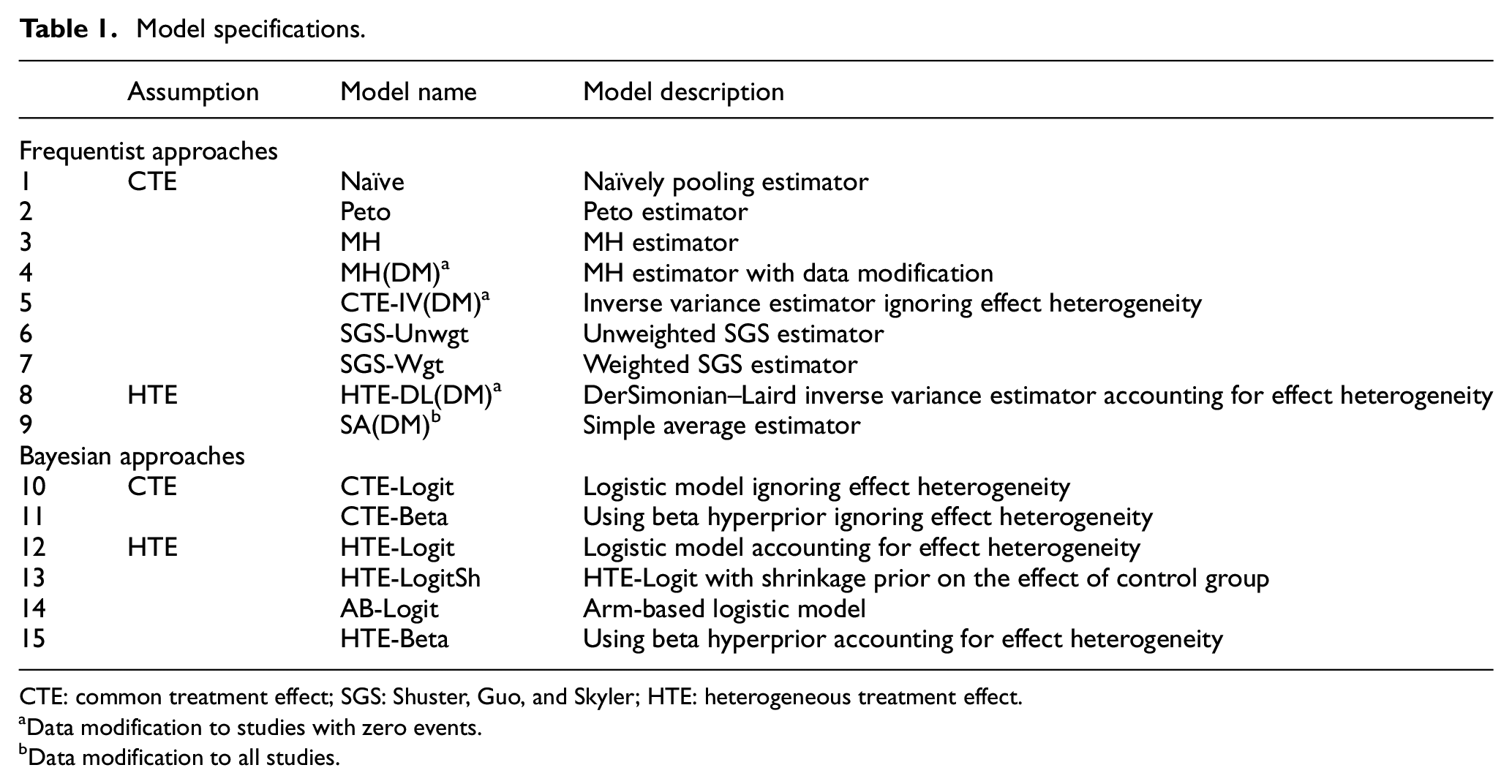
CTE: common treatment effect; SGS: Shuster, Guo, and Skyler; HTE: heterogeneous treatment effect.

Data modification to studies with zero events.

Data modification to all studies.

With binary data, each study in a meta-analysis forms a 2 × 2 table as in Table 2. Here, i indexes study ( $i = 1, \dots, M$ , where M is the number of studies), and k indexes treatment with $k = 1$ for control and $k = 2$ for the treated group. We assume that the outcomes follow a binomial distribution

y_{ik} ~ Bin (n_{ik}, p_{ik})

(1)

Table 2.

Data structure for study i.

	No. of events	No. of non-events	Total
Active treatment	$y_{i 2}$	$n_{i 2} - y_{i 2}$	$n_{i 2}$
Control treatment	$y_{i 1}$	$n_{i 1} - y_{i 1}$	$n_{i 1}$
Total	$y_{i \cdot}$	$n_{i \cdot} - y_{i \cdot}$	$n_{i \cdot}$

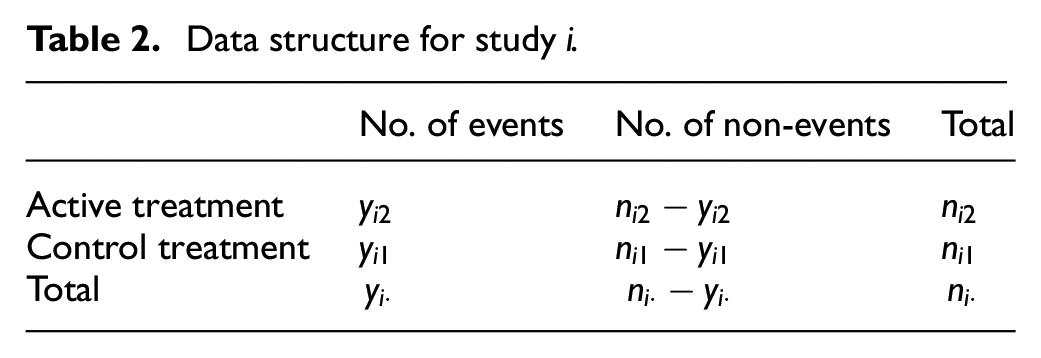
where for the kth treatment in the ith study, $y_{ik}$ is the number of events, $n_{ik}$ is the number of subjects receiving treatment k, and $p_{ik}$ is the probability of having an event.

Frequentist meta-analysis models

Naïve estimator

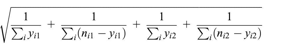
We first consider an estimator that naïvely pools multiple contingency tables, without accounting for effect heterogeneity across studies (denoted by “Naïve”). The naïve LOR estimator is written as

{\hat{LOR}}_{naive} = \log \frac{{\hat{p}}_{2} (1 - {\hat{p}}_{1})}{{\hat{p}}_{1} (1 - {\hat{p}}_{2})}

(2)

where ${\hat{p}}_{1} = \frac{\sum_{i} y_{i 1}}{\sum_{i} n_{i 1}}$ and ${\hat{p}}_{2} = \frac{\sum_{i} y_{i 2}}{\sum_{i} n_{i 2}}$ . The standard error of ${\hat{LOR}}_{naive}$ is calculated as

\sqrt{\frac{1}{\sum_{i} y_{i 1}} + \frac{1}{\sum_{i} (n_{i 1} - y_{i 1})} + \frac{1}{\sum_{i} y_{i 2}} + \frac{1}{\sum_{i} (n_{i 2} - y_{i 2})}}

Peto and Mantel-Haenszel estimators

Peto¹⁸ and Mantel-Haenszel¹⁹ estimators assume CTE across studies (denoted by “Peto” and “MH” respectively). The Peto estimator and its variance are

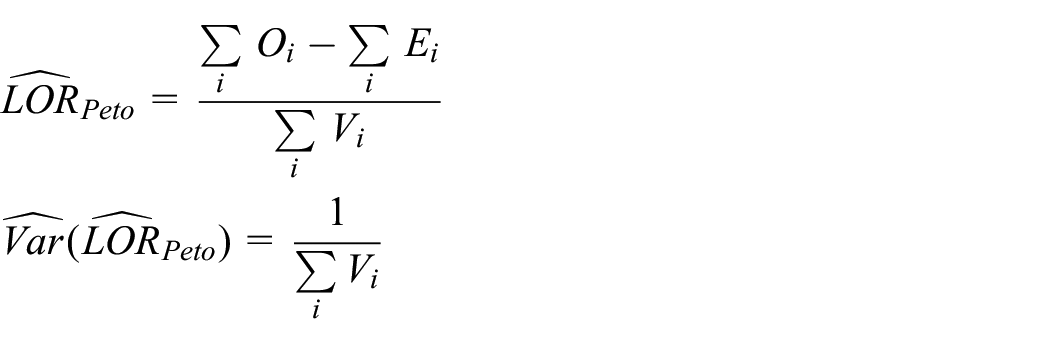
\begin{matrix} {\hat{LOR}}_{Peto} = \frac{\sum_{i} O_{i} - \sum_{i} E_{i}}{\sum_{i} V_{i}} \\ \hat{Var} ({\hat{LOR}}_{Peto}) = \frac{1}{\sum_{i} V_{i}} \end{matrix}

where $O_{i} = y_{i 2}$ , $E_{i} = \frac{y_{i \cdot} n_{i 2}}{n_{i \cdot}}$ , $V_{i} = \frac{y_{i \cdot} n_{i 1} n_{i 2} (n_{i \cdot} - y_{i \cdot})}{n_{i \cdot}^{2} (n_{i \cdot} - 1)}$ , $n_{i \cdot} = n_{i 1} + n_{i 2}$ , and $y_{i \cdot} = y_{i 1} + y_{i 2}$ .

The Mantel-Haenszel estimator and its approximate variance proposed by Robins et al.²⁰ can be written as

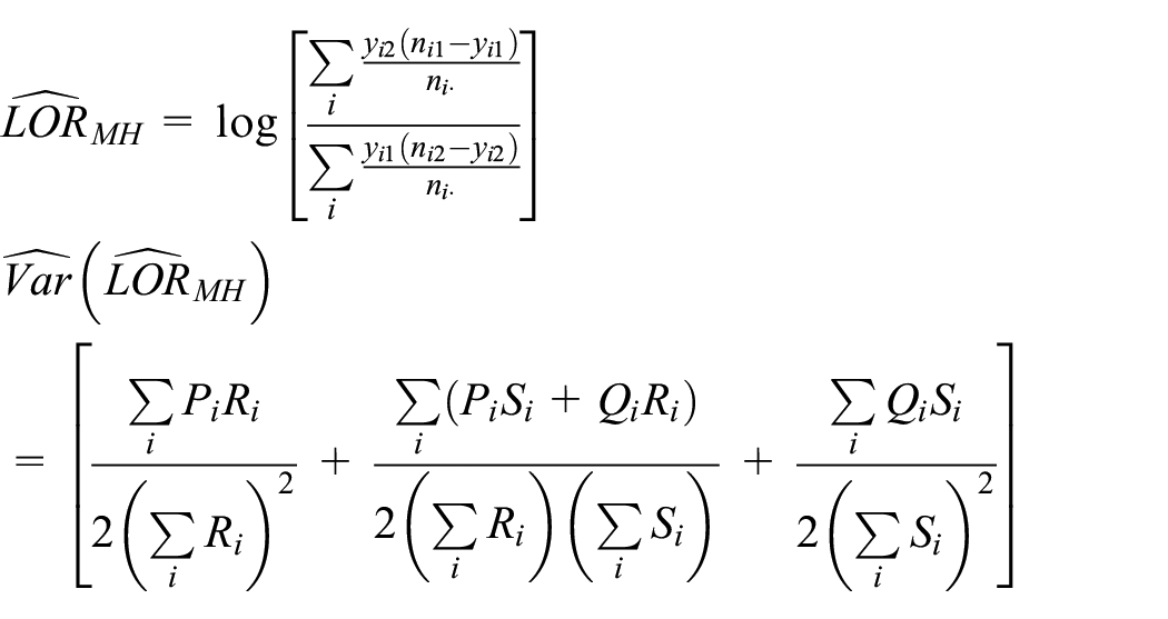
\begin{matrix} {\hat{LOR}}_{MH} = \log [\frac{\sum_{i} \frac{y_{i 2} (n_{i 1} - y_{i 1})}{n_{i \cdot}}}{\sum_{i} \frac{y_{i 1} (n_{i 2} - y_{i 2})}{n_{i \cdot}}}] \\ \hat{Var} ({\hat{LOR}}_{MH}) \\ = [\frac{\sum_{i} P_{i} R_{i}}{2 {(\sum_{i} R_{i})}^{2}} + \frac{\sum_{i} (P_{i} S_{i} + Q_{i} R_{i})}{2 (\sum_{i} R_{i}) (\sum_{i} S_{i})} + \frac{\sum_{i} Q_{i} S_{i}}{2 {(\sum_{i} S_{i})}^{2}}] \end{matrix}

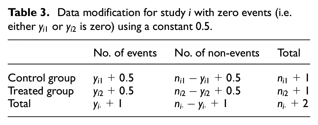
where $R_{i} = \frac{y_{i 2} (n_{i 1} - y_{i 1})}{n_{i \cdot}}$ , $S_{i} = \frac{y_{i 1} (n_{i 2} - y_{i 2})}{n_{i \cdot}}$ , $P_{i} = \frac{y_{i 2} + n_{i 1} - y_{i 1}}{n_{i \cdot}}$ , and $Q_{i} = \frac{y_{i 1} + n_{i 2} - y_{i 2}}{n_{i \cdot}}$ .

Studies with zero cells are not a problem for the Peto and Mantel-Haenszel estimators because they do not calculate the observed LORs of the individual studies. Nevertheless, a data modification that adds a constant 0.5 to all cells of the 2 × 2 table for a trial with zero events in either group as in Table 3 is often considered with the Mantel-Haenszel estimator. We denote the Mantel-Haenszel estimator with data modification by “MH(DM).” A few alternative data modification approaches have been proposed by Sweeting et al.⁹

Table 3.

Data modification for study i with zero events (i.e. either $y_{i 1}$ or $y_{i 2}$ is zero) using a constant 0.5.

	No. of events	No. of non-events	Total
Control group	$y_{i 1} + 0.5$	$n_{i 1} - y_{i 1} + 0.5$	$n_{i 1} + 1$
Treated group	$y_{i 2} + 0.5$	$n_{i 2} - y_{i 2} + 0.5$	$n_{i 2} + 1$
Total	$y_{i \cdot} + 1$	$n_{i \cdot} - y_{i \cdot} + 1$	$n_{i \cdot} + 2$

Inverse variance estimators

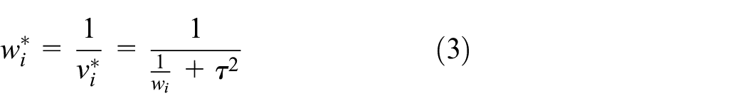
The inverse variance method²¹ is commonly used in meta-analysis. This method can assume either CTE or HTE. When HTE is assumed, we follow DerSimonian and Laird (DL)²¹ to estimate effect heterogeneity, $τ_{DL}^{2}$ (i.e. between-study variances of LOR). First, we need to calculate a study-specific weight $w_{i}^{*}$ as a combination of within-study and between-study variances. Suppose ${\hat{LOR}}_{i} = \log (\frac{y_{i 2} (n_{i 1} - y_{i 1})}{y_{i 1} (n_{i 2} - y_{i 2})})$ then

w_{i}^{*} = \frac{1}{v_{i}^{*}} = \frac{1}{\frac{1}{w_{i}} + τ^{2}}

(3)

where $1 / w_{i}$ is the within-study variance (i.e. the variance of ${\hat{LOR}}_{i}$ ) and $τ^{2}$ is the between-study variance. We estimate $τ^{2}$ using $τ_{DL}^{2}$ as follows

{\hat{τ}}_{DL}^{2} = {\begin{matrix} \frac{Q - df}{C}, & if Q > df \\ 0, & if Q \leq df \end{matrix}

(4)

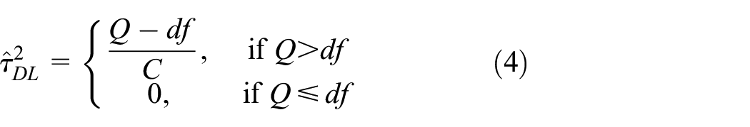
where df is the number of studies minus 1, $Q = \sum_{i} w_{i} ({\hat{LOR}}_{i} - \hat{LOR})^{2}$ , $\hat{LOR} = \frac{\sum_{i} w_{i} {\hat{LOR}}_{i}}{\sum_{i} w_{i}}$ , and $C = \sum_{i} w_{i} - \frac{\sum_{i} w_{i}^{2}}{\sum_{i} w_{i}}$ . As a result, the inverse variance estimator and its variance are written as

\begin{matrix} {\hat{LOR}}_{IV} = \frac{\sum_{i} w_{i}^{*} {\hat{LOR}}_{i}}{\sum_{i} w_{i}^{*}} \\ \hat{var} ({\hat{LOR}}_{IV}) = \frac{1}{\sum_{i} w_{i}^{*}} \end{matrix}

We apply the data modification approach introduced in the previous section to the inverse variance method to handle zero events. Under the CTE assumption, we force $τ^{2}$ in equation (3) to be zero and denote this estimator by “CTE-IV(DM).” We denote the estimator that uses ${\hat{τ}}_{DL}^{2}$ to account for HTE as “HTE-DL(DM).”

Other estimators

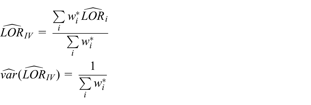
Shuster, Guo, and Skyler (SGS)¹¹ proposed estimators that are the functions of risk estimates in each group. These estimators are non-parametric and assume independence between studies, an assumption called studies at random. They proposed unweighted and weighted estimators, denoted by “SGS-Unwgt” and “SGS-Wgt,” respectively, for odds ratio (OR), risk ratio, and risk difference scales.

For these estimators, one first estimates study-specific risks as ${\hat{p}}_{ik} = y_{ik} / n_{ik}$ and then calculates summary estimates of group-specific risks as ${\hat{π}}_{k} = \sum_{i} {\hat{p}}_{ik} / M$ , where M is the number of studies. The unweighted log odds ratio estimator is given by $\log (\frac{{\hat{π}}_{2} (1 - {\hat{π}}_{1})}{{\hat{π}}_{1} (1 - {\hat{π}}_{2})})$ . The weighted log odds ratio estimator applies study-specific weights, $u_{i} = (n_{i 1} + n_{i 2}) / 2$ , to the study-specific risk estimates for group k, ${\hat{p}}_{ik}$ . One then calculates the estimator from the weighted study group-specific estimates as with the unweighted estimator. They provided formulas for standard errors of the unweighted and weighted estimators.¹¹ We note that their unweighted estimator weights all studies equally, regardless of study sizes, while their weighted estimator weights each study by the study’s total sample size.

Bhaumik et al.¹⁰ proposed a simple average estimator. It is calculated as an average of study-specific LORs after adding 0.5 to all cells in Table 2 for all trials. That is, the study-specific log odds ratio is

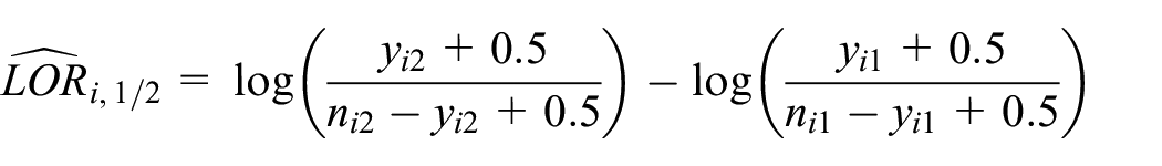
{\hat{LOR}}_{i, 1 / 2} = \log (\frac{y_{i 2} + 0.5}{n_{i 2} - y_{i 2} + 0.5}) - \log (\frac{y_{i 1} + 0.5}{n_{i 1} - y_{i 1} + 0.5})

Then, the simple average estimator and its variance are defined as

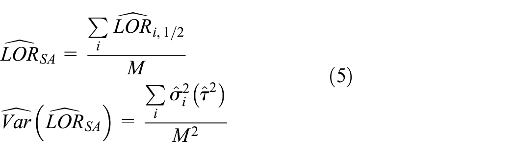
\begin{matrix} {\hat{LOR}}_{SA} = \frac{\sum_{i} {\hat{LOR}}_{i, 1 / 2}}{M} \\ \hat{Var} ({\hat{LOR}}_{SA}) = \frac{\sum_{i} {\hat{σ}}_{i}^{2} ({\hat{τ}}^{2})}{M^{2}} \end{matrix}

(5)

where M is the number of studies, ${\hat{σ}}_{i}^{2} ({\hat{τ}}^{2}) = {[n_{i 1} {\hat{p}}_{i 1} (1 - {\hat{p}}_{i 1})]}^{- 1} + {[n_{i 2} {\hat{p}}_{i 2} (1 - {\hat{p}}_{i 2})]}^{- 1} + {\hat{τ}}^{2}$ , and ${\hat{p}}_{ik} = \frac{y_{ik} + 0.5}{n_{ik} + 1}$ for k = 1 and 2. We use ${\hat{τ}}_{DL}^{2}$ in equation (4) in the variance estimator (5). Note that this estimator uses a data modification that is different from the one used with the Mantel-Haenszel and inverse variance estimators. We denote the simple average estimator by “SA(DM).”

Bayesian meta-analysis models

Logistic regression

Using the likelihood (1), we model the unknown parameter $p_{ik}$ as follows

CTE - Logit : logit (p_{ik}) = μ_{i} + dI (k = 2)

(6)

HTE - Logit : logit (p_{ik}) = μ_{i} + δ_{i} I (k = 2)

(7)

where $μ_{i}$ is the study-specific baseline effect (i.e. log odds of control group) and $I (\cdot)$ is the indicator function. Under the common treatment effect assumption in equation (6), d is the assumed common log odds ratio between the two k groups (control and treated) across studies. We assign vague $N (0, 10^{2})$ priors to $μ_{i}$ and d and denote this model by “CTE-Logit.”

Under the heterogeneous treatment effect assumption in equation (7), $δ_{i}$ is the study-specific log odds ratio. We assume $δ_{i} ~ N (d, τ^{2})$ a priori, where $τ$ quantifies between-study effect heterogeneity, and d has a vague $N (0, 10^{2})$ prior. We assume a $Uniform (0, 2)$ prior distribution for $τ$ , where the range of this uniform prior makes it considerably vague, relative to the scale of the log odds ratio. We consider two priors for $μ_{i}$ : vague and shrinkage priors (denoted by “HTE-Logit” and “HTE-LogitSh,” respectively). The HTE-Logit model assigns a vague $N (0, 10^{2})$ prior to $μ_{i}$ . The HTE-LogitSh sets $μ_{i} ~ N (m, τ_{μ}^{2})$ , where m is the overall mean log odds of the event in the control group, and $τ_{μ}$ is the heterogeneity of the log odds across the studies’ control groups. We set $m ~ N (0, 10^{2})$ and $τ_{μ} ~ Uniform (0, 2)$ , so that the shrinkage prior allows study-specific baseline effects $(μ_{i})$ and log odds ratios $(δ_{i})$ to vary across studies.

Arm-based model

Recently, Hong et al.²² proposed an arm-based parameterization in network meta-analysis, an extension of meta-analysis to compare more than two treatments simultaneously. We simplify this model to fit an arm-based meta-analysis. This model estimates the treatment-specific risks and allows heterogeneity across studies. The model can be written as

logit (p_{ik}) = θ_{k} + η_{ik}

(8)

where $θ_{k}$ is the log odds of treatment k and the $η_{ik}$ is the random effects allowing heterogeneity of the log odds. We assume that $(η_{i 1}, η_{i 2})^{T} ~ BVN ((0, 0)^{T}, Σ)$ where BVN stands for bivariate normal distribution. We use priors $θ_{k} ~ N (0, 10^{2})$ and $Σ^{- 1} ~ Wishart (Ω, 2)$ , where $Ω$ is a $2 \times 2$ matrix resulting in a vague prior for $Σ^{- 1}$ . Note that the choice of $Ω$ depends on data, outcomes, and scales of parameters of interest. We used a diagonal matrix with diagonal elements equal to 0.02 for simulated data and 0.25 for data analysis. One can obtain log odds ratio from $θ_{2} - θ_{1}$ . We call this model “AB-Logit.”

Beta hyperprior distribution

We also consider pooling studies’ arm-specific risks using beta hyperprior distributions. First, we assume that the probability of having an event with treatment k is constant across studies. For the likelihood, we replace $p_{i 1}$ and $p_{i 2}$ in equation (1) with $p_{1}$ and $p_{2}$ , such as

y_{ik} ~ Bin (n_{ik}, p_{k})

Then, we assign prior distributions $p_{k} ~ Beta (α_{k}, β_{k})$ , where $α_{k}$ and $β_{k}$ are pre-specified. We employ common $α$ and $β$ values instead of $α_{k}$ and $β_{k}$ for simplicity, given that we use $Beta (1, 1)$ priors. We call this model “CTE-Beta.”

We also assume heterogeneity across studies, that is, the $p_{ik}$ varies across studies. We define a hierarchical prior distribution for the $p_{ik}$ , namely

p_{ik} ~ Beta (U_{k} V_{k}, (1 - U_{k}) V_{k})

(9)

With this notation, $E (p_{ik} | U_{k}, V_{k}) = U_{k}$ and $Var (p_{ik} | U_{k}, V_{k}) = \frac{U_{k} (1 - U_{k})}{V_{k} + 1}$ . In terms of the more common $Beta (a_{k}, b_{k})$ parameterization, $U_{k} = \frac{a_{k}}{a_{k} + b_{k}}$ and $V_{k} = a_{k} + b_{k}$ . We use this parameterization because we want to assign a prior distribution directly to the mean of $p_{ik} s$ , which is $U_{k}$ . Study heterogeneity in the probability scale is measured by $\frac{U_{k} (1 - U_{k})}{V_{k} + 1}$ . We assign $V_{k}$ a vague prior, namely Inverse-Gamma(1, 0.01). $U_{k}$ has a $Beta (1, 1)$ prior distribution. We call this model “HTE-Beta.”

Bayesian model comparison

We compare the performance of fitted Bayesian models in our data example using the Watanabe–Akaike or widely applicable information criterion.²³ This criterion evaluates predictive accuracy for a fitted model and then adjusts for overfitting based on the effective number of parameters. In addition, it provides more stable estimates than the deviance information criterion. One prefers models that have smaller values of Watanabe–Akaike information criterion.²⁴

Computation

Simulation studies and data analyses were conducted in R.²⁵ We fit the Peto, Mantel-Haenszel, and inverse variance estimators using the R package metafor;²⁶ we used user-written functions to compute the remaining frequentist estimators. Bayesian models were fitted using the R package R2jags²⁷ for simulations and Rstan²⁸ for the data analysis, as Rstan provided reliable Watanabe–Akaike information criterion values. For Bayesian models, a total of 10,000 posterior samples were used after a 10,000 burn-in from a single Markov chain for our simulation studies, while our data analyses used two Markov chains, with each chain having a total of 30,000 posterior samples after a 20,000 burn-in. We checked trace plots and scatter plots of pairs of parameters to ensure convergence; they converged well. The R code and the associated Bayesian model files are available at https://github.com/HwanheeHong/MetaAnalysis_RareEvents.

Simulation study

Settings

In this simulation study, we compare the performance of 15 meta-analysis methods (9 frequentist and 6 Bayesian), summarized in Table 1. The results compare bias, mean squared error, and coverage probability of 95% intervals for each method’s LOR estimate. The simulation settings and results with relative risk and risk difference scales are presented in Supplementary Material.

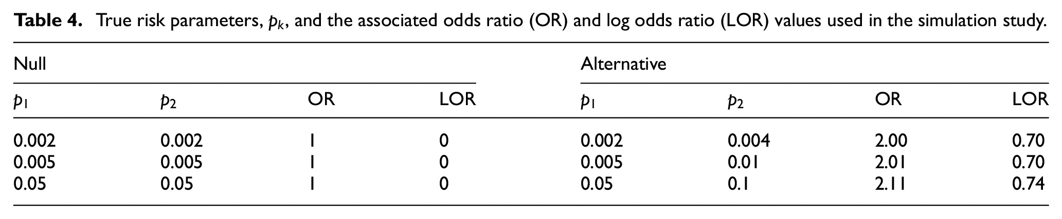
Our simulation setup is built upon that used in Shuster et al.¹¹ We generated 10,000 simulated meta-analysis datasets, each consisting of 30 studies comparing a treatment of interest to a control. The control group’s sample size in study i, $n_{i 1}$ , is sampled from a $Uniform (50, 1000)$ distribution. We set the size of the corresponding treated group, $n_{i 2}$ , to be equal to $n_{i 1}$ to avoid an unrealistic study design that has extremely unbalanced sample sizes. We sampled probabilities for having an event (i.e. risks) for the two groups in study i as follows: $p_{ik} ~ Uniform (p_{k} (1 - 0.5 D), p_{k} (1 + 0.5 D))$ . $p_{k}$ is the true risk for group k = 1 or 2, and D controls between-study heterogeneity of the risks. Table 4 shows the six pairs of true underlying risks that we consider in our six different simulation scenarios. We vary $p_{k}$ to consider three null cases, namely, $(p_{1}, p_{2}) = (0.002, 0.002)$ , $(0.005, 0.005)$ , and $(0.05, 0.05)$ , and three alternative cases, $(p_{1}, p_{2}) = (0.002, 0.004)$ , $(0.005, 0.01)$ , and $(0.05, 0.1)$ . The true log odds ratios are 0 and around 0.7 in the null and alternative cases, respectively. As the true risks decrease, the number of studies with zero events increases. For example, the average numbers of studies with zero events in either group over 10,000 iterations were 18, 8, and less than 1 for the three null cases. In addition, we varied the degree of between-study heterogeneity of risks by setting D to 0, 1, or 2, where $D = 0$ means no heterogeneity in risks. As a result, there are $6 \times 3 = 18$ different settings. Given $p_{ik}$ and $n_{ik}$ samples, we generated the binary events as $y_{ik} ~ Binomial (n_{ik}, p_{ik})$ .

Table 4.

True risk parameters, $p_{k}$ , and the associated odds ratio (OR) and log odds ratio (LOR) values used in the simulation study.

Null				Alternative
$p_{1}$	$p_{2}$	OR	LOR	$p_{1}$	$p_{2}$	OR	LOR
0.002	0.002	1	0	0.002	0.004	2.00	0.70
0.005	0.005	1	0	0.005	0.01	2.01	0.70
0.05	0.05	1	0	0.05	0.1	2.11	0.74

Results

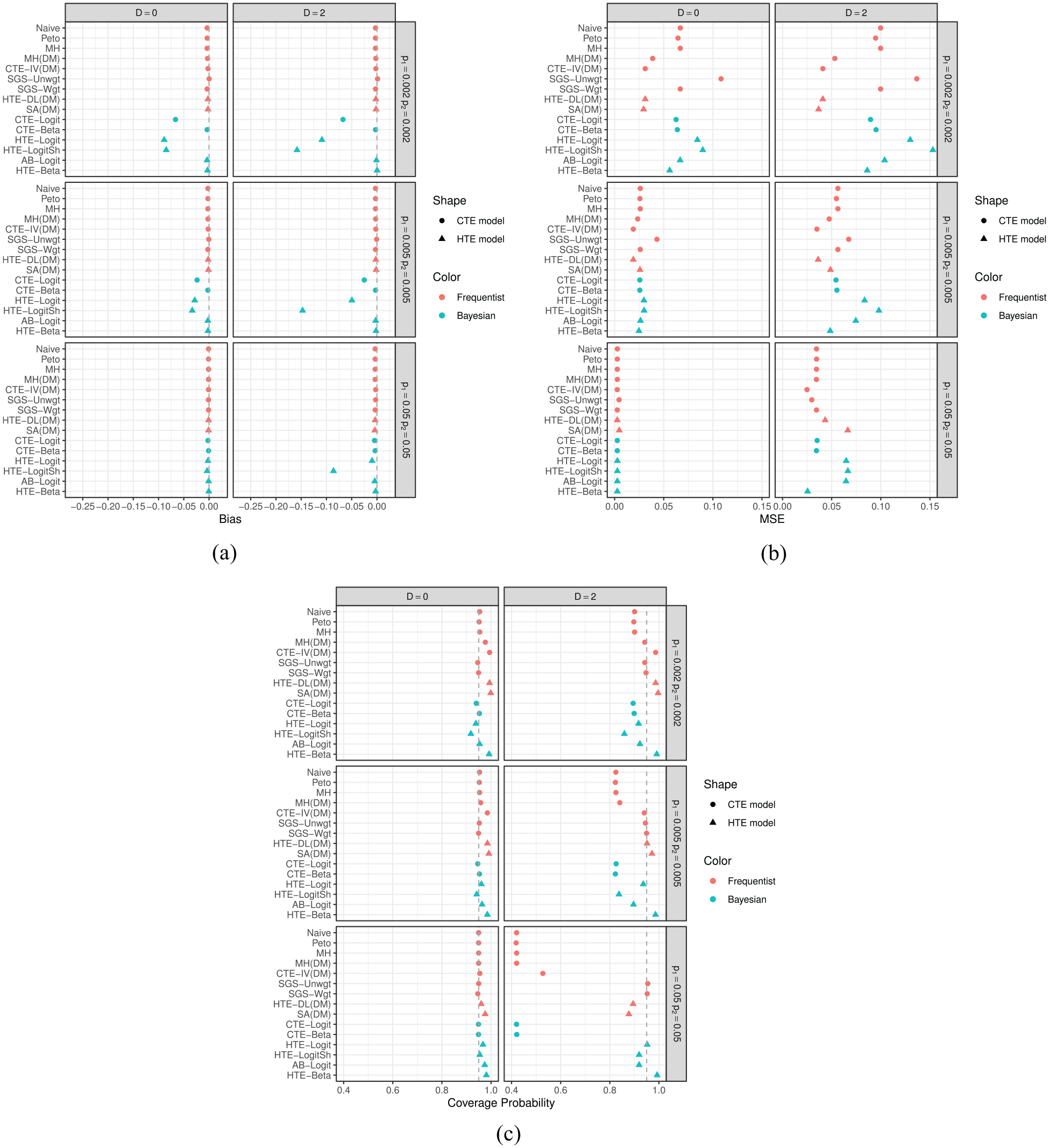
Figures 1 and 2 exhibit bias, mean squared error, and coverage probability of log odds ratio estimates for three null and three alternative cases, respectively. Frequentist and Bayesian models are plotted in red and blue, and common and heterogeneous treatment effect models are plotted using circle and triangle characters, respectively. We present results under $D = 0$ and 2; the results when $D = 1$ are presented in Supplementary Material, as they showed similar patterns to those under $D = 2$ with less extreme quantities.

Figure 1.

Simulation results in the null case: (a) bias, (b) mean squared error, and (c) coverage probability. Frequentist and Bayesian models are plotted in red and blue, respectively; common and heterogeneous treatment effect models are plotted using circles and triangles, respectively.

Figure 2.

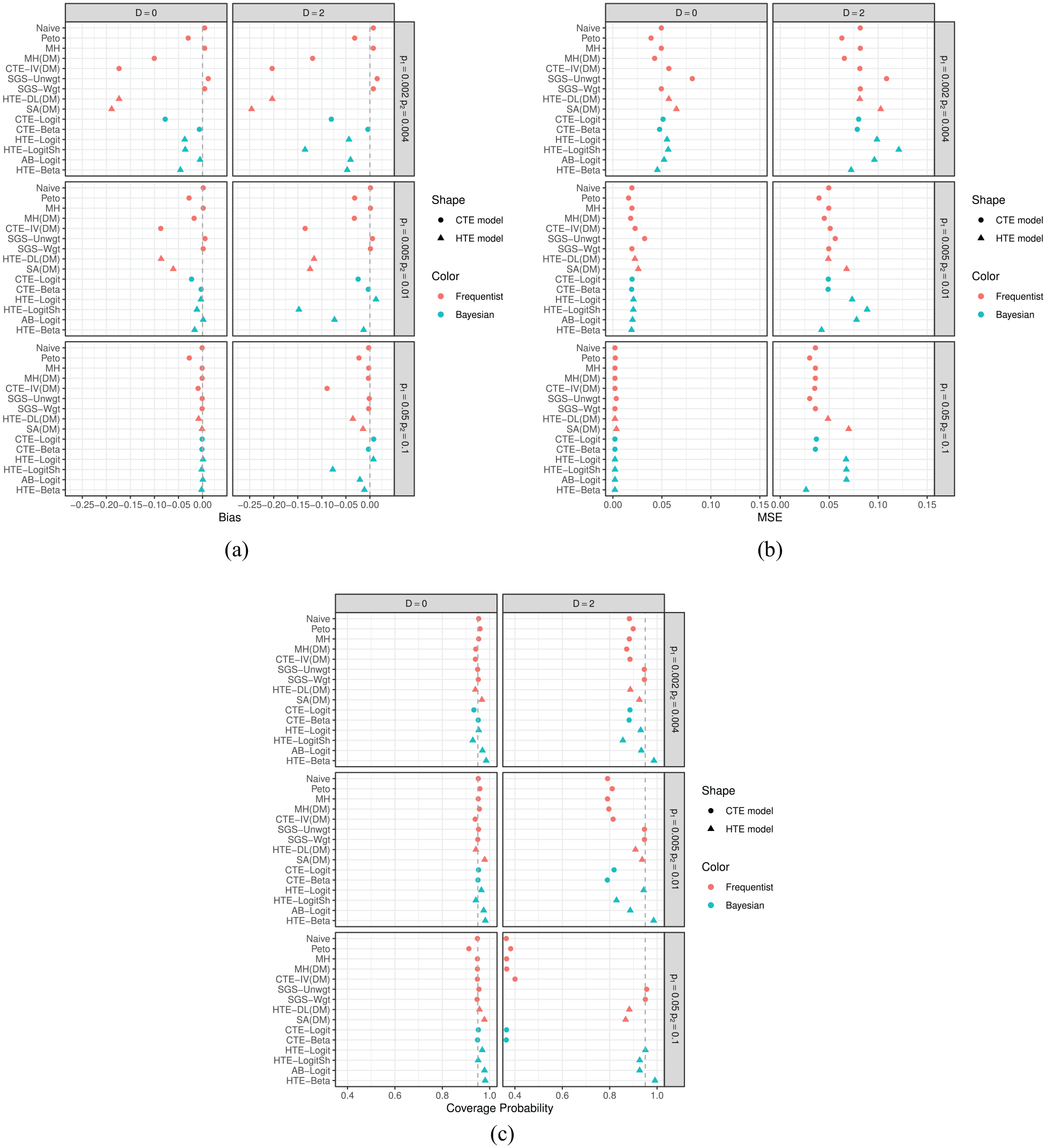
Simulation results in the presence of a treatment effect (i.e. the alternative case): (a) bias, (b) mean squared error, and (c) coverage probability. Frequentist and Bayesian models are plotted in red and blue, respectively; common and heterogeneous treatment effect models are plotted using circles and triangles, respectively.

Under the null cases in Figure 1, all frequentist estimators, which are moment-based estimators, showed little or no bias, as did the three Bayesian methods that model treatment-specific risks, namely CTE-Beta, AB-Logit, and HTE-Beta. CTE-Logit, HTE-Logit, and HTE-LogitSh, however, showed relatively large biases, and the true risks were small. The bias may arise because these three methods rely on a logistic regression model. We generated each meta-analysis dataset from a binomial distribution after we sampled treatment-specific risks, $p_{ik}$ , not treatment effects (i.e. log odds ratios), $δ_{i}$ in equation (7). When the risks are small, studies will have zero cells, making study-specific estimation of the log odds ratio mathematically unwieldy. The estimates across studies become roughly bimodal, with some study estimates around 0 and some approaching infinity. CTE-Logit, HTE-Logit, and HTE-LogitSh model log odds ratio directly under the normality assumption of the $δ_{i}$ , while CTE-Beta, AB-Logit, and HTE-Beta model treatment-specific parameters, such as the log odds of an event. HTE-LogitSh had the largest bias when $D = 2$ , suggesting that a shrinkage normal prior on log odds of an event in the control group may not be appropriate in the presence of large heterogeneity.

Mean squared error decreased as true risks increased (i.e. fewer rare events). When $D = 2$ , MH(DM), CTE-IV(DM), HTE-DL(DM), SA(DM), and HTE-Beta tended to give small mean squared errors, while SGS-Unwgt, HTE-Logit, HTE-LogitSh, and AB-Logit gave large mean squared errors. In terms of coverage probability, SGS-Unwgt, SGS-Wgt, and HTE-Beta provided close to or slightly larger than the nominal level 0.95 across all scenarios. All common treatment effect models, except SGS-Unwgt and SGS-Wgt, had poor coverage in the presence of large between-study heterogeneity $(D = 2)$ , and it got worse as the true risks grew larger. This seemed counterintuitive since all common treatment effect models showed little or no bias in Panel (a). We found that the estimated standard errors of these estimates were so small that their 95% confidence or credible intervals were very narrow, except SGS-Unwgt and SGS-Wgt; the widths of their 95% confidence intervals were sufficiently wider than estimators from the other common treatment effect models that their coverage probabilities were close to the nominal level 0.95.

Figure 2 shows the results for the three alternative cases. The Naïve, Mantel-Haenszel, SGS-Unwgt, SGS-Wgt, CTE-Beta, AB-Logit, and HTE-Beta methods had smaller biases when $D = 0$ and 2. CTE-IV(DM), HTE-DL(DM), and SA(DM) showed large biases when the true risks were small under both $D = 0$ and 2. Again, HTE-LogitSh gave large biases only when $D = 2$ . In terms of mean squared error, four HTE models, SA(DM), HTE-Logit, HTE-LogitSh, and AB-Logit, gave large mean squared error when $D = 2$ , while HTE-Beta and HTE-DL(DM) gave small mean squared error. SGS-Unwgt and SA(DM) had larger mean squared errors in the lowest risk scenario than any other frequentist methods. We see similar results to the null cases in terms of coverage probability.

In the alternative cases, we note two interesting findings that were not observed under the null cases. First, applying the data modification to Mantel-Haenszel resulted in large bias when the true risks were small. That is, adding 0.5 to the contingency table of studies with zero events may bias estimation, especially when a large number of studies report zero events and there is a treatment effect. Second, SGS-Unwgt, SGS-Wgt, and SA(DM) provided very different point estimates, with SA(DM) exhibiting large biases. This discrepancy between the methods may relate to the simulated data generating mechanism being aligned with the SGS-Unwgt and SGS-Wgt estimators’ structure but not that of SA(DM). The target of the SGS-Unwgt and SGS-Wgt estimators is the estimation of treatment-specific risks. These estimators calculate log odds ratio or other treatment effects based on estimates (weighted or unweighted) of treatment-specific risks, ${\hat{p}}_{k}$ . The target parameter of SA(DM), however, is the relative treatment effect, log odds ratio, and it is estimated as an average of study-specific $LO R_{i}$ after applying the data modification to each study’s table.

Rosiglitazone data analysis

The rosiglitazone dataset²⁹ is a popular example with which to study different meta-analysis models with rare events. Many researchers have re-analyzed these data using various methods.^8,30–32 The authors have updated the data by adding a few more relevant trials,³³ and we use these updated data as our real data example. They collected and analyzed these data to investigate the effect of rosiglitazone on the risks of myocardial infarction and of death from cardiovascular causes. There are 56 trials, of which 15 did not report any myocardial infarction, and 29 trials did not report any cardiovascular death in either group.

We apply all models in Table 1 to the rosiglitazone data. For the Bayesian methods, we calculate the Watanabe–Akaike information criterion to compare fitted models. We conducted meta-analyses under four different data settings: (1) include all 56 studies; (2) exclude the RECORD trial, considered as large following Nissen and Wolski³³ (55 studies included); (3) select studies comparing rosiglitazone+X to X alone, where X can be either placebo or an active treatment (42 studies included); and (4) select studies strictly comparing rosiglitazone to placebo (13 studies included). In the 56 studies, the total number of subjects in the rosiglitazone group is 19,509 with 159 (pooled risk = 0.00815) and 105 (0.00538) myocardial infarction and cardiovascular death events, respectively; the total number of subjects in the control group is 16,022, with 136 (0.00848) and 100 (0.00624) myocardial infarction and cardiovascular death events, respectively. We note that the correlation between sample size and observed log odds ratio in each data setting varies from −0.32 to 0.37.

Figure 3 shows the estimated log odds ratios for the four different data settings. log odds ratios less than zero favor rosiglitazone, that is, lower odds of having a myocardial infarction or cardiovascular death event than the control group. For the myocardial infarction outcome, the Peto, Mantel-Haenszel, and SGS-Wgt methods yielded 95% confidence intervals that excluded 0 when all studies were included. 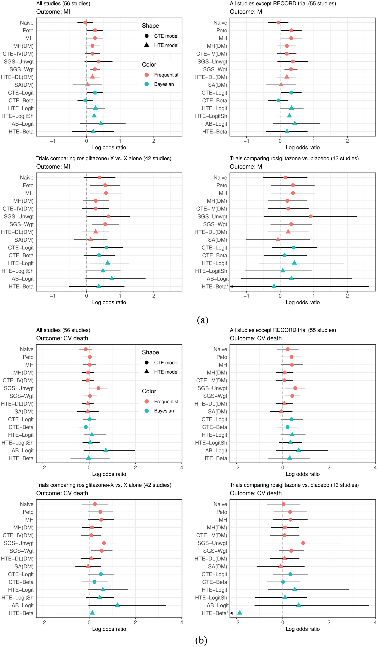The estimated between-study variability in log odds ratio estimates, $\hat{τ}$ , were 0, 0.28, and 0.26 with HTE-DL(DM), HTE-Logit, and HTE-LogitSh, respectively. Note that it is known that frequentist HTE models underestimate effect heterogeneity compared to their Bayesian counterparts.³⁴ Excluding the RECORD trial did not change the point estimates or conclusions much, although the 95% intervals became slightly wider.

Figure 3.

Results of the rosiglitazone data analyses: (a) myocardial infarction and (b) death from cardiovascular causes (CV death). LORs less than zero favor rosiglitazone with lower odds of having an event than control.

When we considered the trials comparing rosiglitazone+X to treatment X alone, the estimated log odds ratios became larger (i.e. stronger effect of rosiglitazone on the odds of having an myocardial infarction event) than those from the other data settings. The Peto, Mantel-Haenszel, SGS-Unwgt, SGS-Wgt, and CTE-Logit methods’ 95% intervals excluded zero. When we included only the 13 studies that compared rosiglitazone to placebo, the associated 95% intervals were wide because of the small number of events: 25 and 14 events out of 7449 and 4860 subjects in the rosiglitazone and placebo groups, respectively. As a result, the HTE-Beta model did not converge and a more informative prior of $V_{k}$ would improve model convergence.

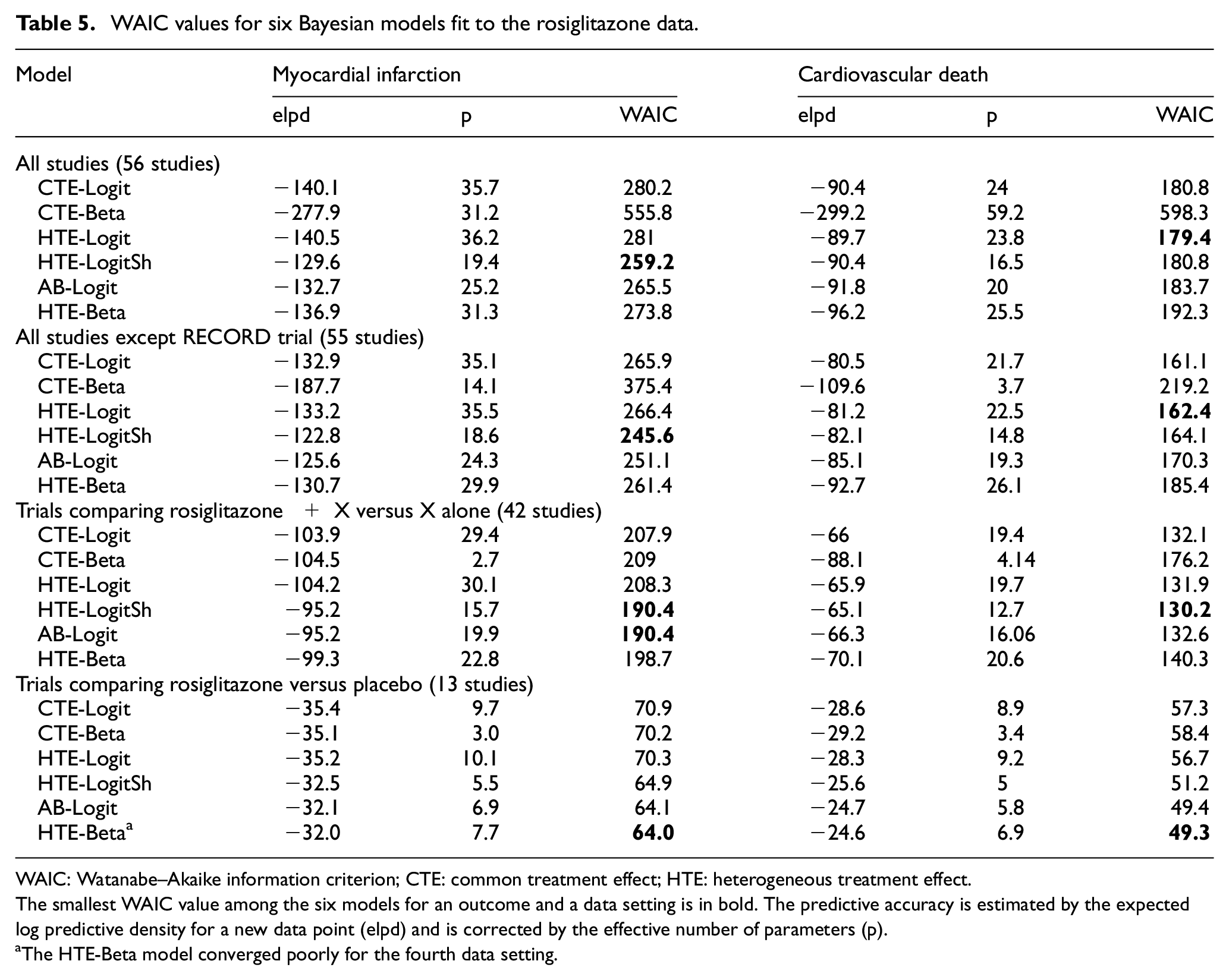
For cardiovascular death, all methods except SGS-Unwgt provided point estimates close to zero and 95% intervals that included zero in the 56-study dataset. The $\hat{τ}$ were 0, 0.41, and 0.34 with HTE-DL(DM), HTE-Logit, and HTE-LogitSh, respectively. Excluding the RECORD trial or comparing rosiglitazone + X to treatment X alone resulted in LOR estimates unfavorable to rosiglitazone, although most 95% intervals included zero; the exceptions were the SGS-Unwgt and SGS-Wgt estimators. When analyzing only the 13 placebo-controlled trials, all frequentist methods provided similar point estimates to the third data setting, except SGS-Unwgt. Again, all methods provided wider 95% intervals and the HTE-Beta model did not converge in this sparse data setting: 11 out of the 13 trials had one or zero cardiovascular death and 4 out of the 11 trials had no events.

Table 5 displays Watanabe–Akaike information criterion values obtained from the six fitted Bayesian models for all outcomes and data settings. For the myocardial infarction outcome, HTE-LogitSh was the best model by the Watanabe–Akaike information criterion for the first three data settings. Although HTE-Beta provided the smallest Watanabe–Akaike information criterion in the fourth setting, when single-agent placebo was the control, the model did not converge. AB-Logit was second place in terms of the Watanabe–Akaike information criterion in each of the data settings. For the cardiovascular death outcome, HTE-Logit (under the first two data settings), HTE-LogitSh (third data setting), and HTE-Beta (fourth data setting) provided the smallest Watanabe–Akaike information criterion values. Again, note that HTE-Beta did not converge in the fourth data setting and AB-Logit provided the second smallest Watanabe–Akaike information criterion value. Across all outcomes and data settings, CTE-Beta provided the largest or second largest Watanabe–Akaike information criterion values, indicating a poor fit to the rosiglitazone data.

Table 5.

WAIC values for six Bayesian models fit to the rosiglitazone data.

Model	Myocardial infarction			Cardiovascular death
Model	elpd	p	WAIC	elpd	p	WAIC
All studies (56 studies)
CTE-Logit	−140.1	35.7	280.2	−90.4	24	180.8
CTE-Beta	−277.9	31.2	555.8	−299.2	59.2	598.3
HTE-Logit	−140.5	36.2	281	−89.7	23.8	179.4
HTE-LogitSh	−129.6	19.4	259.2	−90.4	16.5	180.8
AB-Logit	−132.7	25.2	265.5	−91.8	20	183.7
HTE-Beta	−136.9	31.3	273.8	−96.2	25.5	192.3
All studies except RECORD trial (55 studies)
CTE-Logit	−132.9	35.1	265.9	−80.5	21.7	161.1
CTE-Beta	−187.7	14.1	375.4	−109.6	3.7	219.2
HTE-Logit	−133.2	35.5	266.4	−81.2	22.5	162.4
HTE-LogitSh	−122.8	18.6	245.6	−82.1	14.8	164.1
AB-Logit	−125.6	24.3	251.1	−85.1	19.3	170.3
HTE-Beta	−130.7	29.9	261.4	−92.7	26.1	185.4
Trials comparing rosiglitazone + X versus X alone (42 studies)
CTE-Logit	−103.9	29.4	207.9	−66	19.4	132.1
CTE-Beta	−104.5	2.7	209	−88.1	4.14	176.2
HTE-Logit	−104.2	30.1	208.3	−65.9	19.7	131.9
HTE-LogitSh	−95.2	15.7	190.4	−65.1	12.7	130.2
AB-Logit	−95.2	19.9	190.4	−66.3	16.06	132.6
HTE-Beta	−99.3	22.8	198.7	−70.1	20.6	140.3
Trials comparing rosiglitazone versus placebo (13 studies)
CTE-Logit	−35.4	9.7	70.9	−28.6	8.9	57.3
CTE-Beta	−35.1	3.0	70.2	−29.2	3.4	58.4
HTE-Logit	−35.2	10.1	70.3	−28.3	9.2	56.7
HTE-LogitSh	−32.5	5.5	64.9	−25.6	5	51.2
AB-Logit	−32.1	6.9	64.1	−24.7	5.8	49.4
HTE-Beta^a	−32.0	7.7	64.0	−24.6	6.9	49.3

WAIC: Watanabe–Akaike information criterion; CTE: common treatment effect; HTE: heterogeneous treatment effect.

The smallest WAIC value among the six models for an outcome and a data setting is in bold. The predictive accuracy is estimated by the expected log predictive density for a new data point (elpd) and is corrected by the effective number of parameters (p).

The HTE-Beta model converged poorly for the fourth data setting.

Discussion

We considered many different meta-analytic models when the outcome event is rare. We assessed and compared the performance of frequentist and Bayesian approaches through an extensive simulation study under various data generating settings. The simulations considered really low frequency to somewhat rare event risks and examined no between-study heterogeneity to large heterogeneity. We also fitted all models to the rosiglitazone data and compared the Bayesian models using the Watanabe–Akaike information criterion.

Our simulation results suggest that we should interpret results of meta-analyses carefully in very low-frequency settings. Overall, HTE-Beta seemed to perform among the best. AB-Logit also performed consistently well across all settings, except for mean squared error when between-study heterogeneity in risks existed. Among moment-based frequentist estimators, the SGS-Unwgt and SGS-Wgt estimators performed well, although the SGS-Unwgt estimator gave relatively large mean squared error under the low-risk settings. The Mantel-Haenszel estimator without a data modification provided no or little bias but had somewhat large mean squared error and under-coverage. Peto performed similarly to Mantel-Haenszel but was slightly more biased than Mantel-Haenszel in the alternative case. All frequentist and Bayesian common treatment effect models, except the SGS-Unwgt and SGS-Wgt estimators, tended to provide poor coverage probabilities when between-study heterogeneity existed.

In our data analyses, log odds ratio estimates and their 95% intervals differed by method. We would not expect all of the methods to be quantitatively the same, but most should be qualitatively similar. If there is great discrepancy across methods, then it may be because of a high degree of study-to-study heterogeneity or correlation between-study design and risks.^5,11 One should investigate the source of such discrepancies, particularly in terms of model goodness of fit. Any method that assumes a common effect across studies may be wrong if there is evidence of a large degree of heterogeneity across studies as, for example, if the studies incorporate different controls.

We noticed a few interesting results in the rosiglitazone data analysis. First, the Naïve and CTE-Beta methods provided similar results because the closed form of the posterior mean of risks for the CTE-Beta model is equivalent to the Naïve pooled risks. Second, CTE-IV(DM) and HTE-DL(DM) provided exactly the same results because the estimated between-study heterogeneity ${\hat{τ}}_{DL} = 0$ with HTE-DL(DM). Third, SGS-Unwgt point and interval estimates were very different from those of SGS-Wgt and gave a totally different conclusion under certain data settings. In the 56-study dataset, SGS-Unwgt indicated an increased risk of cardiovascular death for rosiglitazone with the associated 95% interval that excluded zero, while the SGS-Wgt estimate was close to zero and the associated 95% interval included zero. In addition, these two estimators tended to provide largely different point estimates even with the 13 placebo-controlled trials. Finally, SGS-Unwgt and SA(DM) occasionally provided very different point estimates. The SA(DM) estimator gave estimates close to the null across all data settings with both outcomes, while SGS-Unwgt, with narrow 95% intervals, provided strong evidence of greater risk of an event with rosiglitazone. We observed similar trends in our simulation study, again because the target parameters of these two estimators differ.

Furthermore, the rosiglitazone data analysis showed some findings that differed from what we observed in the simulation study. Simulation study results are valid and applicable to a real data analysis only when the simulation data generating mechanism agrees with the true data generating mechanism of the real data. It is untestable, however, whether the rosiglitazone data follow the same data generating mechanism that we used in our simulation study. Instead, we investigated key empirical features (such as correlation between sample size and risks) in the rosiglitazone data and assessed difference between simulated and real data. First, although our simulation studies suggested that HTE-Beta, AB-Logit, and SGS-Wgt are the generally favored models and HTE-LogitSh may be one of the least favorite models, the Bayesian model comparison using the Watanabe–Akaike information criterion in our rosiglitazone data analysis suggested that HTE-LogitSh was the best fitting model. Second, SGS-Wgt always provided much narrower 95% confidence intervals than SGS-Unwgt. This trend was not observed in our simulations, though. The difference may be because of a non-zero correlation between-study design and observed log odds ratio in the rosiglitazone data, whereas the simulations did not include such correlation. Shuster et al.¹¹ pointed out that SGS-Wgt could be more influenced by large trials than SGS-Unwgt. One advantage of SGS-Wgt, however, is that it tends to have narrower confidence limits as the number of studies increases.

Shuster and Walker⁵ stated two points that need to be considered in meta-analysis methods. One may need to properly handle an interaction between sample size and treatment effect with meta-analysis methods that use weights based on sample sizes, and one may also need to consider the weights as random variables. They argued that most widely used meta-analysis methods with binary outcomes do not consider these two issues. Instead, these methods assume independence of within-study effects and design, called effects at random, and could provide biased estimates. Our simulation study did not address these issues specifically, and further studies are needed.

The rosiglitazone data have flaws that limit the ability to assess if rosiglitazone increases the risks of myocardial infarction and cardiovascular death. A major concern is that it is unclear what the control group is. The dataset includes some studies with active treatments as the control groups and some with placebo controls. Some trials compared rosiglitazone to placebo while a few trials compared rosiglitazone to glyburide. It is questionable whether we can consider placebo and glyburide as comparable control groups. Similarly, it is questionable whether the log odds ratio of rosiglitazone compared to placebo can be combined with log odds ratio of rosiglitazone + X compared to X alone. Nissen and Wolski³³ tackled this issue by providing results from several meta-analyses that included studies having the same comparator (insulin, metformin, sulfonylurea, or placebo). For these specific data, a network meta-analysis may be a more reasonable approach because the data have non-comparable treated and control groups across the trials.²²

Although our findings and discussion were mainly based on the log odds ratio scale, it is important to consider other scales, such as the log relative risk and risk difference, and check the consistency of findings.³⁵ Our simulation and data analysis results with the log relative risk scale were very similar to those for the log odds ratio scale. This is expected as the odds ratio and relative risk are similar numerically for rare events. In our simulations with the risk difference scale, all methods provided very small biases and mean squared errors, but some methods showed poor coverage when outcomes were frequent and heterogeneity was large (see section 2 in Supplementary Material). In the data analysis, the conclusions about treatment effect with risk difference and log odds ratio estimates were the same as those with log odds ratio. Note that reporting both absolute measures (e.g. risk difference) and relative measures (e.g. log odds ratio and log relative risk) might be useful in a meta-analysis that concerns rare events. Absolute measures usually provide a more clinically straightforward interpretation than relative measures, while relative measures tend to have less statistical heterogeneity than absolute measures.³⁵ However, Efthimiou³⁶ warns against use of risk differences when faced with rare events. Bayesian methods are advantageous and flexible when estimating different effect scales and interpreting them based on posterior probabilities.

In summary, when a rare binary event is the outcome of interest, treatment effect estimates obtained from traditional meta-analytic methods may be biased and provide poor coverage probability. This trend worsens when there is large between-study heterogeneity. Effect estimates vary when applying different models and are likely to depend on the characteristics of the data (e.g. level of between-study heterogeneity, rarity of outcomes, correlation between sample size and effect size, and so on). As such, inferences should be drawn cautiously. In general, we recommend methods that focus on first estimating treatment-specific risks and then estimating treatment differences based on summaries of the risks across the studies. Of course, this approach makes most sense when the studies in the meta-analysis share the same treatment and control arms. To avoid making a wrong decision, we recommend fitting various methods, comparing the results and model fit (for Bayesian approaches) and investigating any significant discrepancies across them.

Supplemental Material

sj-pdf-1-ctj-10.1177_1740774520969136 – Supplemental material for Meta-analysis of rare adverse events in randomized clinical trials: Bayesian and frequentist methods

Supplemental material, sj-pdf-1-ctj-10.1177_1740774520969136 for Meta-analysis of rare adverse events in randomized clinical trials: Bayesian and frequentist methods by Hwanhee Hong, Chenguang Wang and Gary L Rosner in Clinical Trials

Footnotes

Acknowledgements

The authors thank for the helpful comments from the Associate Editor and two anonymous reviewers. They also thank Drs Estelle Russek-Cohen and Mark Levenson from the US Food and Drug Administration (FDA) for valuable comments which improved this manuscript.

Declaration of conflicting interests

The author(s) declared no potential conflicts of interest with respect to the research, authorship, and/or publication of this article.

Funding

The author(s) disclosed receipt of the following financial support for the research, authorship, and/or publication of this article: This work was made possible by U01 FD004977-01 from FDA, which supports the Johns Hopkins Center of Excellence in Regulatory Science and Innovation. Its contents are solely the responsibility of the authors and do not necessarily represent the official views of the Department of Health and human services or FDA. Hwanhee Hong was supported by R00MH111807 from the National Institute of Mental Health, and Chenguang Wang and Gary L. Rosner were supported by P30CA006973 from the National Cancer Institute.

ORCID iD

Hwanhee Hong

Supplemental material

Supplemental material for this article is available online.

References

CIOMS Working Group V. Current challenges in pharmacovigilance: pragmatic approaches, https://cioms.ch/wp-content/uploads/2017/01/Group5_Pharmacovigilance.pdf (2001, accessed 24 July 2019).

U.S. Food and Drug Administration. Meta-analyses of randomized controlled clinical trials to evaluate the safety of human drugs or biological products guidance for industry (draft guidance), 2018, https://www.fda.gov/media/117976/download

Stoto

MA.

Drug safety meta-analysis: promises and pitfalls. Drug Saf 2015; 38(3): 233–243.

Bennetts

Whalen

Ahadieh

, et al. An appraisal of meta-analysis guidelines: how do they relate to safety outcomes? Res Synth Methods 2017; 8(1): 64–78.

Shuster

Walker

MA.

Low-event-rate meta-analyses of clinical trials: implementing good practices. Stat Med 2016; 35: 2467–2478.

Bradburn

Deeks

Berlin

, et al. Much ado about nothing: a comparison of the performance of meta-analytical methods with rare events. Stat Med 2007; 26(1): 53–77.

Chakravarty

Levenson

Regulatory issues in meta-analysis of safety data. Quant Eval Saf Drug Dev: Des Anal Report 2014; 67: 237.

Lane

PW.

Meta-analysis of incidence of rare events. Stat Methods Med Res 2013; 22(2): 117–132.

Sweeting

Sutton

Lambert

PC.

What to add to nothing? Use and avoidance of continuity corrections in metaanalysis of sparse data. Stat Med 2004; 23(9): 1351–1375.

10.

Bhaumik

Amatya

Normand

SLT

, et al. Meta-analysis of rare binary adverse event data. J Am Stat Assoc 2012; 107(498): 555–567.

11.

Shuster

Guo

Skyler

JS.

Meta-analysis of safety for low event-rate binomial trials. Res Synth Methods 2012; 3(1): 30–50.

12.

Smith

Spiegelhalter

Thomas

Bayesian approaches to random-effects meta-analysis: a comparative study. Stat Med 1995; 14: 2685–2699.

13.

Sutton

Abrams

KR.

Bayesian methods in meta-analysis and evidence synthesis. Stat Methods Med Res 2001; 10(4): 277–303.

14.

Carlin

Louis

TA.

Bayesian methods for data analysis. 3rd ed. Boca Raton, FL: Chapman & Hall/CRC Press, 2009.

15.

Cai

Parast

Ryan

Metaanalysis for rare events. Stat Med 2010; 29(20): 2078–2089.

16.

Tian

Cai

Pfeffer

, et al. Exact and efficient inference procedure for meta-analysis and its application to the analysis of independent 2×2 tables with all available data but without artificial continuity correction. Biostatistics 2009; 10(2): 275–281.

17.

Rücker

Schwarzer

Carpenter

, et al. Why add anything to nothing? The arcsine difference as a measure of treatment effect in metaanalysis with zero cells. Stat Med 2009; 28(5): 721–738.

18.

Yusuf

Peto

Lewis

, et al. Beta blockade during and after myocardial infarction: an overview of the randomised trials. Prog Cardiovasc Dis 1985; 27(5): 335–371.

19.

Mantel

Haenszel

Statistical aspects of the analysis of data from retrospective studies of disease. J Natl Cancer Inst 1959; 22(4): 719–748.

20.

Robins

Breslow

Greenland

Estimators of the Mantel-Haenszel variance consistent in both sparse data and large-strata limiting models. Biometrics 1986; 42(2): 311–323.

21.

DerSimonian

Laird

Meta-analysis in clinical trials. Control Clin Trials 1986; 7: 177–188.

22.

Hong

Chu

Zhang

, et al. A Bayesian missing data framework for generalized multiple outcome mixed treatment comparisons. Res Synth Methods 2016; 7(1): 6–22.

23.

Watanabe

Asymptotic equivalence of Bayes cross validation and widely applicable information criterion in singular learning theory. J Mach Learn Res 2010; 11: 3571–3594.

24.

Gelman

Hwang

Vehtari

Understanding predictive information criteria for Bayesian models. Stat Comput 2014; 24(6): 997–1016.

25.

R Core Team. R: a language and environment for statistical computing. Vienna: R Foundation for Statistical Computing, 2017, https://www.R-project.org/

26.

Viechtbauer

Conducting meta-analyses in R with the metafor package. J Stat Softw 2010; 36(3): 1–48.

27.

Yajima

R2jags: using R to run “JAGS.” R package version 0.5-7, 2015, https://CRAN.R-project.org/package=R2jags

28.

Stan Development Team. RStan: the R interface to Stan. R package version 2.19.2, 2019, http://mc-stan.org/

29.

Nissen

Wolski

Effect of rosiglitazone on the risk of myocardial infarction and death from cardiovascular causes. N Engl J Med 2007; 356(24): 2457–2471.

30.

Bohning

Mylona

Kimber

Meta-analysis of clinical trials with rare events. Biom J 2015; 57(4): 633–648.

31.

Diamond

Bax

Kaul

Uncertain effects of rosiglitazone on the risk for myocardial infarction and cardiovascular death. Ann Intern Med 2007; 147(8): 578–581.

32.

Friedrich

Beyene

Adhikari

NK.

Rosiglitazone: can meta-analysis accurately estimate excess cardiovascular risk given the available data? Re-analysis of randomized trials using various methodologic approaches. BMC Res Notes 2009; 2(1): 5.

33.

Nissen

Wolski

Rosiglitazone revisited: an updated meta-analysis of risk for myocardial infarction and cardiovascular mortality. Arch Intern Med 2010; 170(14): 1191–1201.

34.

Hong

Carlin

Shamliyan

, et al. Comparing Bayesian and frequentist approaches for multiple outcome mixed treatment comparisons. Med Decis Making 2013; 33(5): 702–714.

35.

CIOMS Working Group X. Evidence synthesis and meta-analysis for drug safety: report of CIOMS Working Group X. Geneva: Council for International Organizations of Medical Sciences (CIOMS), 2016.

36.

Efthimiou

Practical guide to the meta-analysis of rare events. Evid Based Ment Health 2018; 21(2): 72–76.

Supplementary Material

Please find the following supplemental material available below.

For Open Access articles published under a Creative Commons License, all supplemental material carries the same license as the article it is associated with.

For non-Open Access articles published, all supplemental material carries a non-exclusive license, and permission requests for re-use of supplemental material or any part of supplemental material shall be sent directly to the copyright owner as specified in the copyright notice associated with the article.

0.00 MB

0.42 MB