Using multistate models with clinical trial data for a deeper understanding of complex disease processes

Abstract

A clinical trial represents a large commitment from all individuals involved and a huge financial obligation given its high cost; therefore, it is wise to make the most of all collected data by learning as much as possible. A multistate model is a generalized framework to describe longitudinal events; multistate hazards models can treat multiple intermediate/final clinical endpoints as outcomes and estimate the impact of covariates simultaneously. Proportional hazards models are fitted (one per transition), which can be used to calculate the absolute risks, that is, the probability of being in a state at a given time, the expected number of visits to a state, and the expected amount of time spent in a state. Three publicly available clinical trial datasets, colon, myeloid, and rhDNase, in the survival package in R were used to showcase the utility of multistate hazards models. In the colon dataset, a very well-known and well-used dataset, we found that the levamisole+fluorouracil treatment extended time in the recurrence-free state more than it extended overall survival, which resulted in less time in the recurrence state, an example of the classic “compression of morbidity.” In the myeloid dataset, we found that complete response (CR) is durable, patients who received treatment B have longer sojourn time in CR than patients who received treatment A, while the mutation status does not impact the transition rate to CR but is highly influential on the sojourn time in CR. We also found that more patients in treatment A received transplants without CR, and more patients in treatment B received transplants after CR. In addition, the mutation status is highly influential on the CR to transplant transition rate. The observations that we made on these three datasets would not be possible without multistate models. We want to encourage readers to spend more time to look deeper into clinical trial data. It has a lot more to offer than a simple yes/no answer if only we, the statisticians, are willing to look for it.

Keywords

Multistate models clinical trials competing risk disease process intermediate clinical endpoints survival analysis time-to-event data

Introduction

A clinical trial represents a large commitment from all individuals involved, including patients, caretakers, site staff, clinical investigators, and sponsors. It also comes with a huge financial obligation: The median cost of a large phase III trial is $48 million.¹ Given the depth of investment, it is wise to make the most of the data collected by learning as much as possible from it. The premise of this article is to show that multistate models can be a useful tool to achieve that goal.

Randomized controlled trials, specifically, are widely viewed as the gold standard for establishing causal conclusions² since randomization eliminates selection bias and confounding. The primary analysis for such a trial is often tightly focused on a pre-defined hypothesis, and rightfully so. Nevertheless, it would be a missed opportunity if all we learn from a costly clinical trial is a single yes/no answer of whether the new treatment is effective. While it is essential to conduct randomized controlled trials, determine the effectiveness of the new treatment, and bring effective treatment options to patients, we should go beyond that singular purpose and enhance our understanding of the disease process by garnering as much information as possible using clinical trial data. One may argue that most clinical trial analysis plans contain subgroup analysis to explore the treatment effect in specific patient subgroups, but very few explore the richer and more complex relationship among treatment, covariates, and both intermediate and final clinical endpoints, a particular strength of multistate models.

In this article, we showcase the utility of multistate models by demonstrating the additional insight gained from using them with clinical trial data. We use three publicly available clinical trial datasets involving colon cancer, acute myeloid leukemia, and cystic fibrosis from the survival package^3,4 in R, as illustrations.

Multistate models

A multistate model is a generalized framework to describe longitudinal events, and we focus on the multistate hazards (MSH) models in this article. The mathematical roots of MSH are based on counting processes,⁵ which also underlies the Cox model.⁶

The MSH model starts with a state space diagram; a state space for the colon cancer data is shown in Figure 1(a), as an example. Each box is a state, where a patient can reside at a point in time, and each arrow is a possible transition, that is, the direction from one state to another. A transient state means a patient can transition out of that state (e.g. disease-free and recurrence states in Figure 1(a)), whereas a terminal state, also known as an absorbing state, means a transition out of that state is impossible (e.g. death state in Figure 1(a)). A terminal state can be biological, such as death, or it can be due to research interest, for example, in a competing risk model, all states (other than the initial state) are terminal. In MSH models, all states, either transient or terminal, are considered as outcomes; therefore, the effects of treatment and baseline covariates can be evaluated for each transition.

Figure 1.

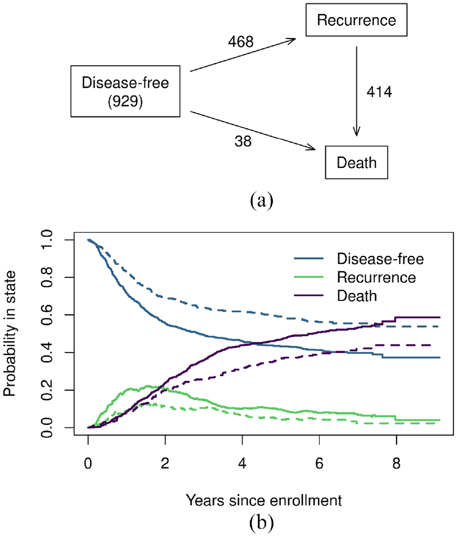
Colon cancer dataset: (a) state space and (b) Aalen-Johansen estimates. (a) Disease free represents patients’ status at trial enrollment. The trial randomized 929 patients, among which 468 experienced recurrence, and 414 subsequently died. There are also 38 patients who died without experience recurrence. (b) The dotted line represents the levamisole+fluorouracil (5FU) arm, and the solid arm represents the control arm. The probability in state sums up to one at a given time, conditional on the treatment. For example, at year 4, the probability in state for disease-free, recurrence, and death are 46%, 10%, and 44%, respectively, for patients in the control arm.

An MSH model analysis consists of two elements:

Fit the per transition proportional hazards models. These models are analogous to Cox models where one model is fitted for each transition.

a. The input dataset for the MSH model follows the counting process format. Each row of data contains an identifier, a “start time,” an “end time,” and a “status” variable. For example, the data below show patient 1 who enrolled on day 0, experienced disease recurrence on day 968, and subsequently died on day 1521. Patient 2 was followed up for 3087 days without recurrence or death. Details on how to construct a dataset in counting process format, the requirements for a counting process dataset, and how to ensure that the dataset is created correctly are provided in the Supplemental Material.

id time1 time2 state

1 0 968 recur

1 968 1521 death

2 0 3087 censor

b. MSH model can also incorporate time-varying covariates with ease. The covariate value, in the counting process dataset, represents the covariate value for the time interval. If the covariate value changes, then additional rows of data should be created.

c. The MSH model is flexible where each transition can have its own set of covariates. An example of how to carry this out is included in the colon cancer data.

Calculate absolute risks which include the following quantities.

a. $p_{k} (t; x)$ , the probability of being in state $k$ at time $t$ , given a baseline covariate vector $x$ . $p_{k} (t; x)$ should sum up to one across the $k$ state $s$ given $x$ .

b. $E (N_{k} (t; x))$ , the expected number of visits to state $k$ by time $t$ , given a baseline covariate vector $x$ .

c. $RMT S_{k} (t; x)$ , the expected amount of time spent in state $k$ by time $t$ , given a baseline covariate vector $x$ . It is known as the restricted mean time in state in multistate analysis literature. It is also known as the restricted mean survival time in survival literature or sojourn time in the field of stochastic processes.

The absolute risk values can be estimated using the non-parametric Aalen-Johansen estimator,⁷ a generalization of the Kaplan-Meier estimator⁸ to multiple outcomes, when there are no covariates present, or as predictions from the MSH model, analogous to the Breslow estimate^9,10 from a Cox model. For readers who are interested in learning more about multistate models, a good introduction to the methods can be found in the tutorial article by Putter et al.¹¹ The book by Cook and Lawless¹² provides a more technical background.

In the remainder of this article, we focus on using MSH models to estimate the transition rate and absolute risk while adjusting for covariates. We will use three clinical trial datasets as examples to demonstrate that the hazard ratios and absolute risks provide complementary information in an MSH model and shed light on the complex relationship between treatment, intermediate clinical endpoints, and baseline covariates. The R codes used to generate all the figures and results are provided in the Supplemental Material.

Colon cancer data

Description

These are data from one of the first successful trials of adjuvant chemotherapy for colon cancer.¹³ The trial enrolled 1296 patients with resected colon cancer with Duke stage B2 or stage C disease. The colon dataset in the survival package^3,4 contains 929 patients with Duke stage C disease who were randomly assigned to observation, levamisole alone (Lev), or levamisole in combination with fluorouracil (Lev+5FU).

For illustration purposes, we collapse observation and Lev arms together as a control arm since there is no difference across these two arms in disease-free survival (Supplemental Figure 1). We also chose to use age (in years), gender (male vs female), node4 (>4 vs ≤4 positive lymph nodes), and extent (extent of local spread, 1 to 4) for modeling where the extent variable is treated as a continuous variable.

The colon cancer data are used to demonstrate how to carry out a MSH model analysis, what quantities can be estimated and their interpretations, and how to perform checks for assumptions.

Results

Figure 1(a) shows the state space for the colon cancer trial; among the 929 patients in the trial, 423 (46%) experienced neither event, and very few patients (N = 38) went from trial enrollment (disease-free) to death, that is, died without recurrence. We therefore expect the disease-free to death transition to have little effect on the overall results. The Aalen-Johanson estimates (Figure 1(b)) show that most recurrences occurred within 3 years of enrollment, and patients died soon after recurrence, that is, the area under the recurrence curve is small (the area under each curve is an estimate of the sojourn time for that state). The “disease-free” curves show that Lev+5FU is effective since the Lev+5FU curve consistently stays above the control curve.

Figure 2(a) shows the hazard rates from the MSH model. The disease-free to death transition, shown third in the panel, represents the group of patients who died without recurrence, most likely due to non–cancer-related causes; the wide confidence intervals are due to the small number of disease-free to death transitions. Neither the lack of a treatment effect nor the presence of an age effect is surprising for this transition.

Figure 2.

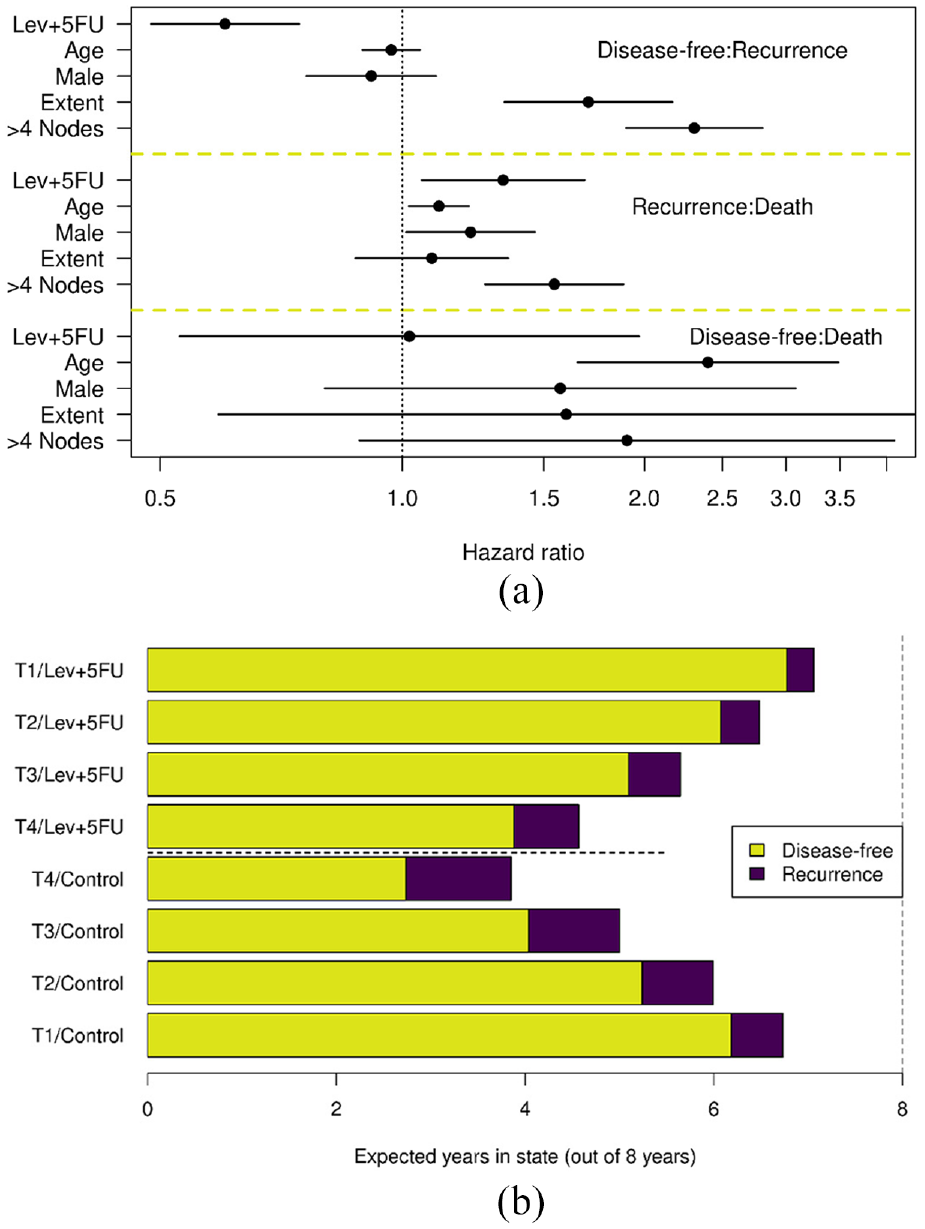
Colon cancer dataset: (a) the multistate hazards model result and (b) the sojourn time. Extent of disease, T1: submucosa, T2: muscle, T3: serosa, T4: contiguous structures. (a) The hazard ratio of age is for “per 10 years increase.” (b) The sojourn time, out of 8 years, in the disease-free (yellow), the recurrence (purple), and death (blank) states by treatment and extent of disease.

Age and sex have essentially no effect on the recurrence rate (i.e. disease-free to recurrence transition). Treatment reduces recurrence rates by about 1.7 (1/0.6) fold. The extent of disease and >4 positive nodes greatly increase the recurrence rate. The disease characteristics of >4 positive nodes and the extent of the disease have similar effects on recurrence and death.

For the recurrence to death transition, age, and gender have small effects, while the effect from >4 positive nodes and the extent of the disease are attenuated. Most interesting is the apparent reversal of the treatment effect, that is, patients who received Lev+5FU died faster after recurrence than those in the control arm. Figure 2(b) shows the sojourn time (out of 8 years) in disease-free and recurrence states by treatment and >4 positive nodes, which helps explain the anomaly. To simplify the figure, the number of positive nodes has been marginalized over, and age/gender were omitted in the model. It is clear that patients who received Lev+5FU have a shorter sojourn time in the recurrence state, in agreement with the hazard ratio shown in Figure 2(a), but it is compensated for by a longer disease-free period (i.e. longer sojourn time in the disease-free state).

The initially puzzling observation of the reversal of treatment effect for the recurrence to death transition now appears to be a classic “compression of morbidity,” proposed by Fries,¹⁴ which hypothesizes that if the age of onset of the first chronic infirmity can be postponed, then the burden of lifetime illness may be compressed into a shorter period before the time of death.¹⁵ The treatment extended time before recurrence, by around 1.2–1.3 years, more than its extension of time before death, by 0.9 and 1 year for ≤4 and >4 nodes, respectively. Therefore, the time spent in recurrence is compressed into a shorter period of time.

An important part of any MSH model, as with a Cox proportional hazards model, is to check the primary model assumptions. This includes proportional hazards, additivity, and functional form. Example codes are included in the Supplemental Material to demonstrate how to perform these checks, as well as how to allow each transition to have its own set of covariates.

This is an example where coupling the hazard ratios from the MSH model with absolute risks provides a fuller understanding of interrelated disease processes.

Myeloid data

Description

CALGB 10603¹⁶ is a randomized phase III clinical trial conducted by the Cancer and Leukemia Group B (CALGB), now part of the Alliance for Clinical Trials in Oncology. This trial evaluated the effect of midostaurin versus placebo, both in combination with daunorubicin and cytarabine, for treatment of newly diagnosed acute myeloid leukemia patients with the fms-related tyrosine kinase 3 gene (commonly known as FLT3) mutation. Patients were randomly assigned to midostaurin versus control while stratifying by their mutation status (tyrosine kinase domain mutation (TKD mutation) vs low-ratio internal tandem duplication (ITD-low) vs high ratio internal tandem duplication (ITD-high)). The study treatment consisted of induction, consolidation, and maintenance phases. Patients were allowed to receive allogeneic hematopoietic stem-cell transplants at the physician’s discretion at any time. A typical treatment pattern is for a patient to be treated until complete response (CR), then the patient may go on to receive further transplant to achieve long-lasting remission. However, since the trial protocol allows transplants at any time, the actual treatment pattern is much more complex, as shown in Figure 3(a). This trial is an example of a complicated treatment and disease process that patients could experience.

Figure 3.

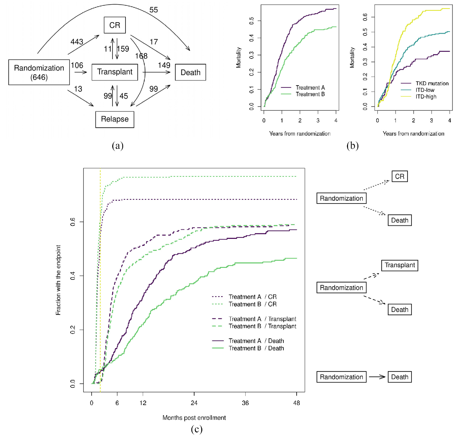
Myeloid dataset: (a) state space, (b) overall survival by treatment and mutation status, and (c) cumulative probability of complete response (CR), transplant, and death. CR: complete response; TKD: tyrosine kinase domain, ITD: internal tandem duplication. (c) The vertical dotted line is the reference line for 2 months. The top right state space represents a competing risk model treating CR and death as competing events which estimates the probability of ever CR. The middle state space represents a competing risk model treating transplant and death as competing events, which estimates the probability of ever receiving transplant. The probabilities of ever CR (dotted lines) and ever receiving transplant (dashed lines) from the two models are overlaid in the same figure while the solid lines represent the probability of death.

The CALGB 10603 and myeloid dataset have been used in prior articles^17,18 that used the Aalen-Johansen estimate to explore patterns of transition with treatment as the only covariate. In this article, we will use MSH models to understand the impact of mutation status on intermediate clinical events, such as CR and transplant. Specifically, concerning CR, we want to know (1) when the extra CR in treatment B occurred, (2) are the extra CR, in treatment B, as durable as the CR in treatment A, and (3) what is the impact of mutation status on whether a patient can obtain CR and the durability of CR. Concerning transplant, we want to know (1) whether there is a difference in transplant rate by treatment, (2) whether there is a difference in the timing of transplant by treatment, and (3) the impact of mutation status on the timing of transplant. To answer these questions, we utilized multiple state spaces where one state space corresponds to one model. The results of these models are overlaid in one figure for ease of visual comparison. The myeloid dataset in the survival package^3,4 is a simulated dataset based on the complex disease process observed in the CALGB 10603 trial. For readers who are interested in the actual CALGB 10603 trial data, please contact the NCTN data archive¹⁹ or Alliance data sharing.²⁰

Results

Figure 3(b) shows the overall survival by treatment and mutation status (the stratification factor used for randomization) in the myeloid dataset. It is evident that both the treatment and mutation status are strongly prognostic.

Figure 3(a) shows all transitions that occurred in the myeloid data. To better understand this complex pattern, we first look at three subsets of the state space: the cumulative probability of ever reaching CR, the cumulative probability of ever receiving a transplant, and the cumulative probability of death. Each of these is an example of an absolute risk, that is, the expected number of visits to a given state. The probability of ever reaching CR and ever receiving a transplant can be obtained by two separate competing risk models; one model treats CR and death as competing events, and another treats transplant and death as competing events.

Figure 3(c) shows the cumulative probability of ever reaching CR, ever receiving a transplant, and death (overlaid in one figure), based on the non-parametric Aalen-Johansen estimate. The majority of the CR events happened between 1 and 2 months (277/454 = 76%); treatment B gains steadily on treatment A from month 2 onward. It also shows most transplants happened after month 2, which is consistent with the clinical practice of transplanting after CR, but there does not appear to be a big difference in transplant rates across treatments. The survival advantage for treatment B begins around month 4, which suggests that it could be at least partially a consequence of the additional CR events. We decided to display the three state spaces alongside the Aalen-Johansen estimates to avoid confusion since we will be using many different state spaces in this example.

CR investigation

An immediate question is whether the “extra” CR events from treatment B are as durable as those from treatment A. To answer this, we use another sub-model with states of randomization, CR, and relapse/death (ignoring transplant) while allowing the CR to relapse/death transition. Figure 4(a) shows the proportion of patients still in CR (solid lines) and the proportion of patients ever in CR (dotted lines) by Aalen-Johansen (overlaid in one figure), and we see that patients departed from the CR state in a similar fashion across treatments. The sojourn time of CR (restricted to 48 months) is 16.3 months and 21.2 months for treatment A versus B, respectively. The additional 4.9 months of CR is statistically significant (p = 0.001). Since the mutation status is a prognostic factor to overall survival, we would like to know whether it impacts CR in the same fashion. Figure 4(b) shows the hazard ratios of the sub-model mentioned earlier. CR in treatment B is indeed durable, supported by the hazard ratio of 0.74 for CR to relapse/death transition. It is interesting that mutation status has minimal effect on the probability of reaching CR, or on the rate of relapse/death without CR, but has a major effect on the transition from CR to relapse/death. This manifests in sojourn time (Table 1) where the sojourn time in the randomization state is more similar across mutation statuses (within a treatment) than the sojourn time in the CR state; patients with TKD mutation have a longer sojourn time in CR than those with ITD-high by about 12 months (consistent across treatments).

Figure 4.

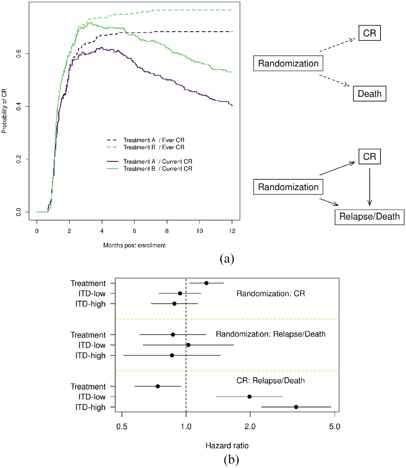
Myeloid dataset: (a) the proportion of ever CR versus current CR and corresponding state space and (b) the multistate hazards model result. CR: complete response; Treatment: treatment B versus treatment A; ITD: internal tandem duplication. (a) The top right state space represents a competing risk model treating CR and death as competing events which estimates the probability of ever CR. The lower right state space allows patients to transition out of CR, therefore estimates the probability of currently in CR. The probabilities of ever CR (dotted lines) and currently in CR (solid lines) from the two models are overlaid in the same figure on the left. (b) For the mutation status, TKD (tyrosine kinase domain) was the reference group in hazard ratio calculation.

Table 1.

Myeloid dataset, estimated sojourn time from a multistate hazards model.

	Sojourn time in randomization state (month)			Sojourn time in CR state (month)
	Treatment A	Treatment B	Difference (B-A)	Treatment A	Treatment B	Difference (B-A)
TKD only	6.4	5.3	–1.1	22.9	27.8	4.9
ITD-low	6.8	5.7	–1.0	16.0	21.2	5.1
ITD-high	8.0	6.7	–1.3	10.8	15.4	4.7

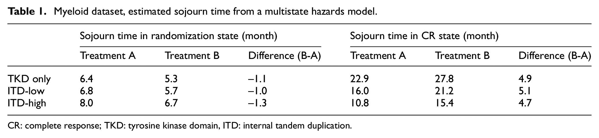
CR: complete response; TKD: tyrosine kinase domain, ITD: internal tandem duplication.

Transplant investigation

A puzzling observation from Figure 3(b) is that if patients received transplants after CR and treatment B have a higher CR probability, why were the transplant curves not different by treatment? Figure 5(a) shows the transplants broken down by whether they happened before or after CR. Most of the transplants without CR happened by month 10 and occurred more often in treatment A. One possible explanation is that once it is apparent to the patient and physician that CR is unlikely, they proceed with the alternative therapy, that is, transplant. The additional CR events on treatment B led to an increase in transplants as well, but at a later time of 12–24 months, that is, for a patient in CR, we can perhaps afford to defer the transplant date. Putting these two observations together, there is no apparent difference in the probability of receiving a transplant between treatments. Figure 5(b) shows the MSH model results where we can see that the mutation status has little or no effect on the rate of randomization to transplant transition (i.e. transplant without CR), but a strong effect on CR to transplant transition (i.e. transplant after CR). This may simply be an aspect of a shorter duration of CR for the more severe mutations, which coincides with what we observed previously. Treatment B has a somewhat lower rate of randomization to transplant transition than treatment A but has no significant effect on the CR to transplant transitions. We can only speculate, but perhaps patients on treatment B were generally “doing well” according to the treating physician’s opinion, that is, patients on treatment B who were not yet declared to be CR were nevertheless less likely to be seen as a clear treatment failure and promoted to an early transplant.

Figure 5.

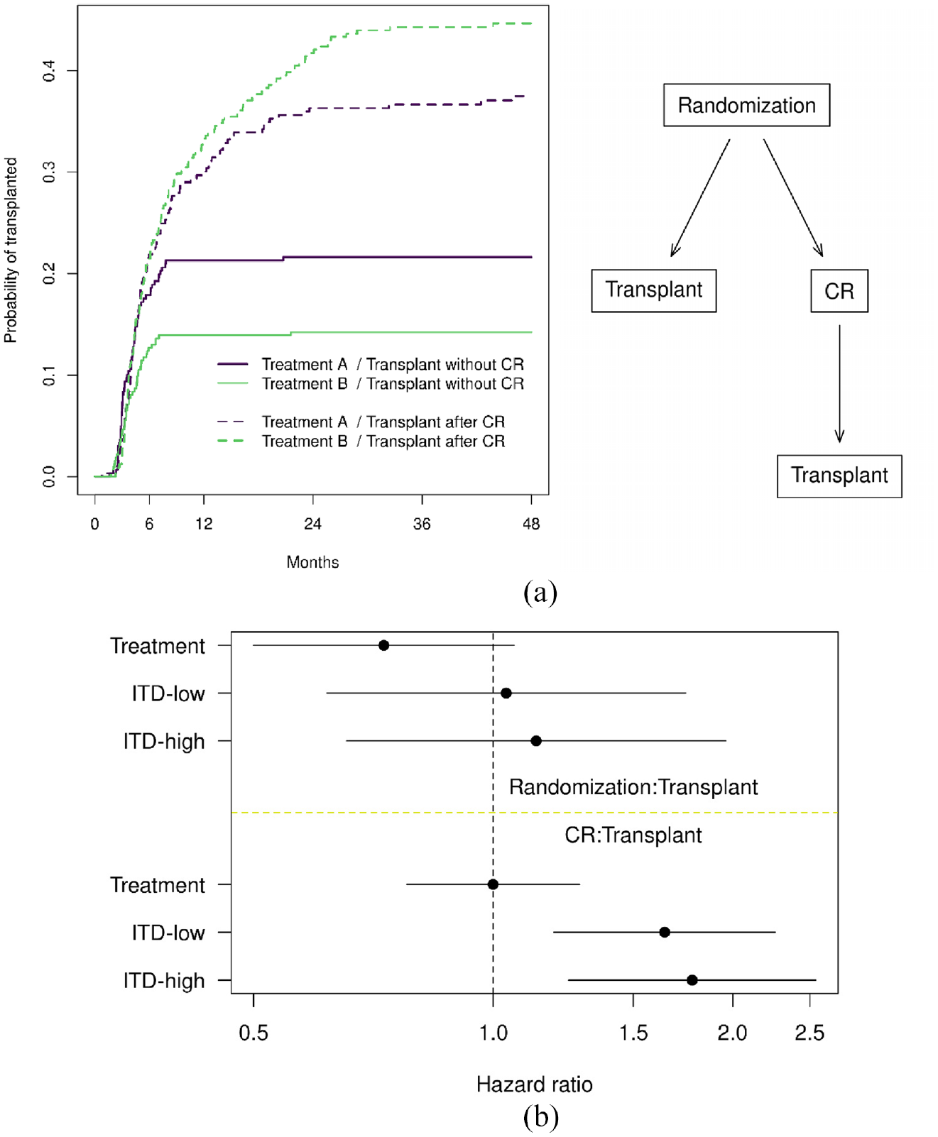
Myeloid dataset: (a) the proportion of transplant without CR and transplant after CR and (b) the multistate hazards model result. Treatment: treatment B versus treatment A; CR: complete response. (a) The dotted lines correspond to the transplant on the right-hand-side split of the state space, and the solid lines correspond to the transplant on the left-hand-side split of the state space. (b) This shows a subset of the multistate hazards model results since we are most interested in these two transitions.

Cystic fibrosis data

Description

The dataset rhDNase contains data from a randomized double-blind clinical trial comparing the efficacy of a highly purified recombinant deoxyribonuclease I (rhDNase) to placebo in patients with cystic fibrosis. Patients can experience repeated events, that is, lung infection, during the follow-up period. The dataset rhDNase is used to demonstrate the following, (1) the ability of the MSH model to handle recurrent events and (2) checks for model assumption; additional details on the data description can be found in the Supplemental Material.

Results

The treatment, rhDNase, and higher baseline lung capacity are both associated with a slower transition from randomization to lung infection and a faster recovery. The detailed results and the code for performing assumptions check are included in the Supplemental Material.

Discussion

The premise of this article is to demonstrate that multistate models are a useful tool and can help us learn more about complex disease processes using clinical trial data. In the colon dataset, a very well-known and well-used dataset, we found that the Lev+5FU substantially delays the onset of recurrence but only modestly increases the longevity, an example of the classic “compression of morbidity.” In the myeloid dataset, we found that CR is durable, patients who received treatment B have longer sojourn time in CR than patients who received treatment A, and the mutation status does not impact the rate to CR but is highly influential on the sojourn time in CR. In addition, we found that more patients in treatment A received transplants without CR, and more patients in treatment B received transplants after CR. The mutation status is also highly influential on the CR–transplant transition rate. The observations that we made on these two datasets would not be possible without multistate models which can treat multiple intermediate/final clinical endpoints as outcomes and estimate the impact of covariates and treatment simultaneously. The cystic fibrosis dataset was used to demonstrate how recurrent events can be handled with MSH models. It is worth noting that MSH models are applicable to not only randomized clinical trials but also longitudinal studies in other disease areas, such as eye disease,^21,22 kidney disease,^23,24 liver disease,^25,26 Alzheimer’s disease,²⁷ and so on.

Since MSH models and Cox models share the same mathematical roots, it is worthwhile to make some connections between the two. The restricted mean time in state is most often known as restricted mean survival time. For a simple two-state alive–dead model, the Aalen-Johansen estimate is equivalent to the Kaplan-Meier estimate, and the probability in state is the Breslow estimate^9,10 of survival based on a Cox model. In addition, since death is an absorbing state, the expected number of visits equals the probability of being in the death state at a given time. It is worth noting that the hazard ratios from a MSH model share the same challenges as a Cox model with respect to using them for causal inference; while the absolute risks are more appropriate to that task.^28,29 Care should still be taken while using absolute risk to establish causal effects since the intermediate endpoints (such as transplant in the myeloid example) are subject to confounders, which may be unmeasurable. For example, it is unlikely to capture the information that influences a physician’s decision on the timing of a transplant; therefore, it will be difficult to obtain unbiased (causal) estimates of the treatment effect on such intermediate endpoints. It is essential to couple the MSH models with the absolute risks to provide a full understanding of the disease process.

For any MSH model, it is critical to use “censoring” only for real censoring (i.e. end of follow-up) and not as a label for any other intermediate clinical endpoints. Using the myeloid dataset as an example, if one wishes to estimate the proportion of patients ever to receive a transplant, a competing risk analysis should be used to treat death as a competing event of transplant. The naïve method of censoring the transplant at the time of death provided a biased result (Supplemental Figure 2). Competing risk analysis is the simplest case, and therefore the one where analysts are most likely to try and shoehorn the data into a method that they are accustomed to (such as the Kaplan-Meier estimator and Cox models), but any MSH model is also prone to the same mistake of treating intermediate clinical endpoints as censoring. We encourage readers to carefully consider the intermediate clinical endpoints and take them into account in the analysis appropriately.

In this article, the time scale that we used is “time after randomization.” Since the clinical trials were designed to answer the question of “whether the new treatment is effective,” randomization represents a natural and appropriate starting time for the analysis. However, for other research questions, for example, evaluating the natural history and progression of age-related conditions, age can serve as an appropriate time scale since it provides a natural interpretation of the analysis results. Choosing the appropriate time scale based on the research questions in hand is an important consideration for multistate models.

For this article, we used the survival package^3,4 in R for the computation. The R code used for the previously detailed analysis is provided as a Supplemental document. The survival package in R is an easy-to-use, well-maintained open-source software with clearly documented vignettes for users. It is, however, not the only tool that readers can use to model the MSH. Other R packages, such as mstate^11,30,31 and msm³² packages, and software programs, such as Stata or SAS, can also be used to carry out the task.

We would like to encourage readers to spend the time and look deeper into their clinical trial data to discover hidden truths about complex disease processes. With appropriate models, the data have a lot more to offer than a simple yes/no answer if only we, the statisticians, are willing to look for it.

Supplemental Material

sj-pdf-1-ctj-10.1177_17407745241267862 – Supplemental material for Using multistate models with clinical trial data for a deeper understanding of complex disease processes

Supplemental material, sj-pdf-1-ctj-10.1177_17407745241267862 for Using multistate models with clinical trial data for a deeper understanding of complex disease processes by Terry M Therneau and Fang-Shu Ou in Clinical Trials

Supplemental Material

sj-pdf-2-ctj-10.1177_17407745241267862 – Supplemental material for Using multistate models with clinical trial data for a deeper understanding of complex disease processes

Supplemental material, sj-pdf-2-ctj-10.1177_17407745241267862 for Using multistate models with clinical trial data for a deeper understanding of complex disease processes by Terry M Therneau and Fang-Shu Ou in Clinical Trials

Footnotes

Declaration of conflicting interests

The author(s) declared no potential conflicts of interest with respect to the research, authorship, and/or publication of this article.

Funding

The author(s) disclosed receipt of the following financial support for the research, authorship, and/or publication of this article: This publication was supported in part by the Daniel J. Sargent, Ph.D., Career Development Award in Cancer Research.

ORCID iD

Fang-Shu Ou

Supplemental material

Supplemental material for this article is available online.

References

Moore

Heyward

Anderson

, et al. Variation in the estimated costs of pivotal clinical benefit trials supporting the US approval of new therapeutic agents, 2015–2017: a cross-sectional study. BMJ Open 2020; 10: e038863.

Hariton

Locascio

JJ.

Randomised controlled trials—the gold standard for effectiveness research: study design: randomised controlled trials. BJOG 2018; 125(13): 1716.

Therneau

TM.

A package for survival analysis in R. 3.1-12 ed. Vienna: R Core Team, 2023.

Therneau

Grambsch

PM.

Modeling survival data: extending the Cox model. New York: Springer, 2000.

Andersen

Borgan

Gill

, et al. Statistical models based on counting processes. New York: Springer Science & Business Media, 2012.

Cox

Regression models and life tables. J R Stat Soc Series B (Methodol) 1972; 34: 187–220.

Aalen

Johansen

Empirical transition matrix for nonhomogeneous Markov-Chains based on censored observations. Scand J Stat 1978; 5: 141–150.

Kaplan

Meier

Nonparametric estimation from incomplete observations. J Am Stat Assoc 1958; 53: 457–481.

Breslow

. Contribution to the discussion on the paper by D. R. Cox, regression models and life tables. J R Stat Soc Series B 1972; 34: 216–217.

10.

Lin

DY.

On the Breslow estimator. Lifetime Data Anal 2007; 13: 471–480.

11.

Putter

Fiocco

Geskus

RB.

Tutorial in biostatistics: competing risks and multi-state models. Stat Med 2007; 26: 2389–2430.

12.

Cook

Lawless

JF.

Multistate models for the analysis of life history data. London: Chapman & Hall/CRC Press, 2018.

13.

Moertel

Fleming

Macdonald

, et al. Levamisole and fluorouracil for adjuvant therapy of resected colon carcinoma. N Engl J Med 1990; 322: 352–358.

14.

Fries

JF.

Aging, natural death, and the compression of morbidity. N Engl J Med 1980; 303: 130–135.

15.

Swartz

James Fries: healthy aging pioneer. Am J Public Health 2008; 98(7): 1163–1166.

16.

Stone

Mandrekar

Sanford

, et al. Midostaurin plus chemotherapy for acute myeloid leukemia with a FLT3 mutation. N Engl J Med 2017; 377: 454–464.

17.

Le-Rademacher

Peterson

Therneau

, et al. Application of multi-state models in cancer clinical trials. Clin Trials 2018; 15(5): 489–498.

18.

Le-Rademacher

Therneau

FS.

The utility of multistate models: a flexible framework for time-to-event data. Curr Epidemiol Rep 2022; 9(3): 183–189.

19.

National Cancer Institute. NCTN/NCORP data archive, https://nctn-data-archive.nci.nih.gov/ (accessed 17 December 2023).

20.

The Alliance for Clinical Trials in Oncology. Data sharing requests, https://www.allianceforclinicaltrialsinoncology.org/main/public/standard.xhtml?path=%2FPublic%2FDatasharing (accessed 17 December 2023).

21.

Kinoshita

Yokota

Mieno

, et al. Multi-state model for predicting ocular progression in acute Stevens-Johnson syndrome/toxic epidermal necrolysis. PLoS ONE 2021; 16(12): e0260730.

22.

Gangnon

Lee

Klein

, et al. Severity of age-related macular degeneration in 1 eye and the incidence and progression of age-related macular degeneration in the fellow eye: the Beaver Dam Eye Study. JAMA Ophthalmol 2015; 133(2): 125–132.

23.

Lintu

Shreyas

Kamath

A multi-state model for kidney disease progression. Clin Epidemiol Glob 2022; 13: 100946.

24.

Lyons

Mody

Bewley

, et al. Multistate modeling of clinical trajectories and outcomes in the ICU: a proof-of-concept evaluation of acute kidney injury among critically ill patients with COVID-19. Crit Care Explor 2022; 4(12): e0784.

25.

Allen

Therneau

Larson

, et al. Nonalcoholic fatty liver disease incidence and impact on metabolic burden and death: a 20 year-community study. Hepatology 2018; 67(5): 1726–1736.

26.

Jepsen

Ott

Andersen

, et al. Risk for hepatocellular carcinoma in patients with alcoholic cirrhosis. Ann Intern Med 2012; 156: 841–847.

27.

Jack

Jr Therneau

Lundt

, et al. Long-term associations between amyloid positron emission tomography, sex, apolipoprotein E and incident dementia and mortality among individuals without dementia: hazard ratios and absolute risk. Brain Commun 2022; 4(2): fcac017.

28.

Hernan

MA.

The hazards of hazard ratios. Epidemiology 2010; 21: 13–15.

29.

Aalen

Cook

Røysland

Does Cox analysis of a randomized survival study yield a causal treatment effect. Lifetime Data Anal 2015; 21(4): 579–593.

30.

de Wreede

Fiocco

Putter

mstate: an R package for the analysis of competing risks and multi-state models. J Stat Softw 2011; 38: 1–30.

31.

de Wreede

Fiocco

Putter

The mstate package for estimation and prediction in non- and semi-parametric multi-state and competing risks models. Comput Methods Programs Biomed 2010; 99(3): 261–274.

32.

Jackson

CH.

Multi-state models for panel data: the msm package for R. J Stat Softw 2011; 38: 1–28.

Supplementary Material

Please find the following supplemental material available below.

For Open Access articles published under a Creative Commons License, all supplemental material carries the same license as the article it is associated with.

For non-Open Access articles published, all supplemental material carries a non-exclusive license, and permission requests for re-use of supplemental material or any part of supplemental material shall be sent directly to the copyright owner as specified in the copyright notice associated with the article.

0.00 MB

0.41 MB

0.42 MB