
Abstract
Most sales forecasts, including those in the generic drug industry, are based on an implicit assumption that the market can be represented as a continuous variable, an approach that works only when activity consists of many independent, incremental customer buying decisions, each of which is too small to substantially affect total sales. These conditions are generally true in branded pharmaceutical markets but they do not reflect the reality of the US generic drug industry where decisions regarding which company’s product is dispensed at the pharmacy are primarily a function of a limited number of binary (yes/no) decisions from drug wholesaling companies, the largest of which control access to one-fourth of the market or more. Unfortunately, binary situations are difficult to model in standard spreadsheet forecasts due to the extremely high number of permutations that are possible even with a small number of variables. In this paper, we explore the binary nature of the US multi-source industry from a single, hypothetical, generic company’s perspective and discuss a probability-based sales forecasting technique that offers a more accurate approach to modeling based on the number of wholesaler contracts available and the degree of generic competition present. The forecast is derived from actual wholesaler market share data and, based on extensive industry experience, the parameters used are believed to be reasonably representative of the US generic market, meaning that the results can be scaled to determine approximate probabilities of achieving certain revenue levels in real-world situations.
Keywords
Introduction
Although they may not be consciously aware of it, marketers and market forecasters tend to think in terms of continuous variables. For example, when someone asks the value of 1, 5, or 10 share points, they are operating on an unstated assumption that a product’s share can take any value between zero and one. This assumption holds true in markets made up of many independent, incremental customer buying decisions, each of which is too small to substantially affect total sales. With some caveats, it is a reasonable representation of the brand drug environment where activity is composed of numerous, independent prescribing decisions made by a large number of physicians, any one of whom represents a small portion of the overall business.
There are, however, many situations where the assumptions required for continuous variable modeling do not hold up. One relatively well-known example is the market for large passenger airliners where manufacturers compete for just a small number of high-value contracts from the handful of global airlines that need and can afford new airplanes. In such cases, rather than using a continuous variable approach, market share needs to be modeled as the combined outcome of n binary (yes/no) decisions where n is the number of potential contracts available.
Based on our experience, the market for generic drugs in the United States is, if anything, more binary in nature than the commercial airliner industry. The reason for this is that, while physicians choose which active ingredient gets prescribed, the company whose product gets dispensed at the pharmacy is a function of decisions made by a very small number of large wholesalers and pharmacy chains. A single one of these buyers might control 25% or more of a market and, with the exception of very high-volume generics, these purchasers tend to select a single primary supplier who will get all or nearly all of that company’s business.
As a result, models suggesting that generic business can be won or lost in single or half share point increments are unrealistic. They are also potentially dangerous in that they underestimate the importance of every single purchase decision: a brand drug company that lost the business of the category’s highest prescribing physician would not suffer nearly the same impact as a generic company that lost a major distributor contract. To ensure that this reality is represented, forecasters need to construct models that accurately simulate a small number of binary rather than a large number of continuous buying decisions.
Standard spreadsheet models are problematic for binary modeling of this type. For example, think of a situation where buying decisions are made independently by five distributors, each of which controls access to a different percentage of the market. Each distributor will also award a primary and secondary contract meaning that there are a total of 10 contracts being put out for bid (again, with each representing a different level of business for the winner). Even in a relatively simple example like this, the generic supplier faces 1024 potential primary–secondary/win–loss outcomes. When we consider that a forecaster using a regular spreadsheet would have to change each variable individually and record the results of each permutation, we can start to see why handling the bidding process as a continuous variable is a more common approach; it is much easier to judge the outcome of an additional share point than to run through all the binary permutations. Fortunately, the use of probability-based techniques such as Monte Carlo analysis (MCA) allow forecasters to construct the model and then rely on computing power to calculate the outcomes of the various permutation. To illustrate how vast the differences between a continuous and binary variable approach can be in markets that have a small number of buyers, our company did just that. The results are discussed below.
Structure of US pharmaceutical distribution
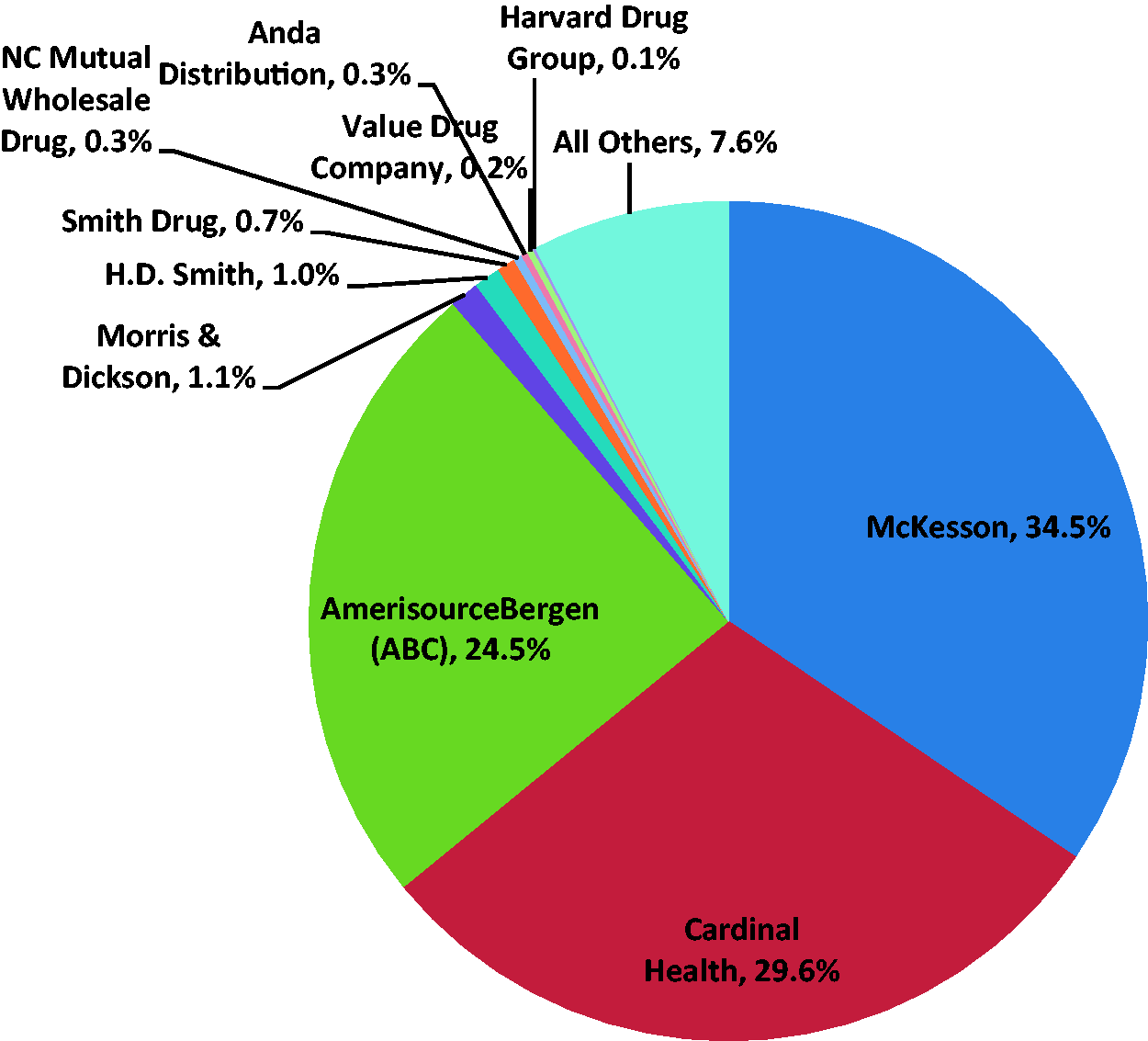
Figure 1 below shows US pharmaceutical wholesaler market share as of 2011. It clearly demonstrates the disparity between the conditions for use of a continuous variable-based forecast (i.e. many independent, incremental buying decisions, each of which is too small to substantially affect total sales) and the reality faced by generic drug companies (i.e. three wholesalers controlling almost 90% of the market and large number of very small companies servicing the other 10%).
US pharmaceutical distribution: market share by wholesaler, 2011.
1
Modeling generic drug sales
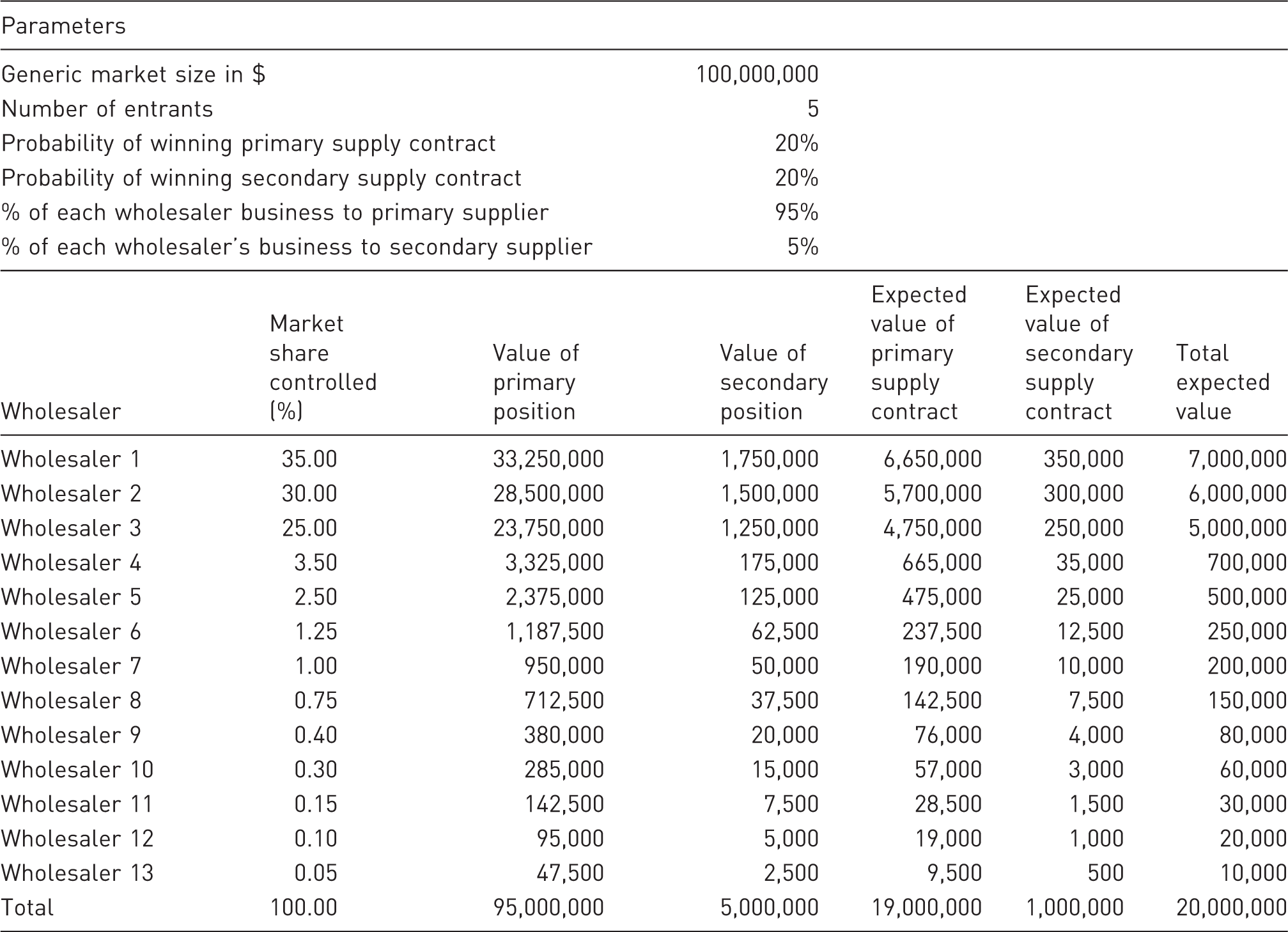
Based on the data in Figure 1, we constructed a standard spreadsheet model with the following parameters:
There are 13 wholesalers in total. The top three companies control 35%, 30%, and 25% of the market, respectively (90% collectively). The remaining 10% of the market is controlled by 10 smaller wholesalers. The largest has 3.5% of the market and the smallest has 0.1%. This is a modest simplification for modeling purposes; in fact, as Figure 1 illustrates, there are an unspecified number of very small wholesalers (i.e. less than 0.2% of the market) that are collectively responsible for 7.6% of US drug distribution.
Other parameters of the model are as follows:
The generic molecule under consideration has combined (all entrants) sales of US$100 million annually. Each entrant has an equal chance of winning contracts. For example, if there are two entrants, the probability of winning is 50%; with three entrants, the probability of winning is 33.3%; with four entrants, 25%, etc. Each wholesaler offers a primary contract and a secondary contract. The primary contract will get 95% of that company’s business, and the secondary contract will receive the remaining 5%. Generic suppliers can only win one contract per wholesaler (i.e. they cannot win both the primary and secondary spots), and they will always accept the better contract (i.e. if they win the primary, they take themselves out of the running for the secondary).
Initial generic drug sales forecast (expected value method)
About probability-based forecasting
Having seen why the continuous variable and expected value approaches are unsuited for generic drug sales forecasting, we will now demonstrate why probability-based methods are more appropriate for the task. Toward this end, a little background on MCA is in order. Readers who are more interested in how the structure of the wholesaler system affects generic sales than in the mechanics of the modeling process may wish to skip ahead to the “Forecast results” section.
As we know, standard spreadsheet models provide a single figure or figures representing what is believed to be the most likely outcome. No matter how well-built the model or how high the quality of data used, the probability of getting the same results in the real world is extremely low (and sometimes, as we have seen in the preceding example, mathematically impossible). In recognition of this, many models also include best- and worst-case scenarios. However, the boundaries for these scenarios tend to be arbitrarily selected and assume that everything will go right or everything will go wrong—again, a rare outcome in reality.
Unlike these techniques, MCA replaces single-point estimates with probability distribution functions, thereby allowing for realistic incorporation of risk and uncertainty into forecasting models. After probability distributions have been assigned to the parameters, the model is then calculated and recalculated hundreds or thousands of times, with each iteration having a different set of randomly generated values derived from the probability functions. As these randomly generated distribution values interact with each other, they ripple throughout the model showing outcomes for the entire spectrum of possible outcomes. The results provide decision-makers with a wide range of feasible outcomes and their probabilities of occurrence.
Expressed a little differently, spreadsheets allow us to change one variable at a time in order to assess its impact on the model: for example, “what happens if we raise the price 5%?” In contrast, MCA changes all the variables simultaneously on each iteration: for example, “what happens if we raise the price 5% and price sensitivity is 2% higher than we expected and the economy enters a recession?” The next iteration might answer the question: “what happens if we raise the price 3% and price sensitivity is 10% lower than expected and the economy experiences flat growth?” This process is repeated over and over again until all feasible values and combinations of values have been tested and recorded for analysis.
Simple MCAs can be performed by using Microsoft Excel’s RAND and RANDBETWEEN functions in combination with other standard formulas. For example, the binary analysis described below could be performed by using RAND to generate a random number between 0 and 1; in a separate cell, an IF statement could be written that returns a value of 0 or 1 depending on the value of the randomly generated number. Assuming that there is a 25% probability of winning a contract, then the IF cell would return 1 if the randomly generated value was less than or equal to 0.25 and 0 if the value was greater than 0.25. Similar formulas would be constructed for each of the available contracts, the 0 and 1 contract win values would be multiplied by the value of each contract, etc. Additional IF statements could be added to reflect the modeling rules that allow for suppliers to win only one contract per wholesaler and preference for larger over smaller contracts.
This approach would represent a single iteration of the model which is of limited value in a Monte Carlo context; it is akin to determining the probability distribution of a coin toss by flipping the coin once. This problem can be overcome by copying the formulas hundreds or thousands of times and then analyzing the results in the aggregate. Although this would not be particularly difficult with the current scenario, commercially available software packages that work as spreadsheet add-ins are recommended for more complex modeling scenarios.
Creating the probability-based model
The modeling parameters are left unchanged in the MCA. To incorporate the probability element, we employed a commercial software package (Palisade Software’s @Risk, which works as an add-in to Microsoft Excel) but the process is similar to the one described above: i.e. a column simulating the binary outcome of each contract was added; the cells in this column can take win (1) or loss (0) values based on the probability of winning each contract. These win/loss results are multiplied by the value of the contract in question, and the sum of contracts won equals the company’s total sales.
To ensure that the probabilities associated with the range of contract win/loss combinations were captured, the model was then run through 10,000 iterations. (Note that each time these iterations return a distinct set of contract wins and losses is equivalent to the results that would be generated by a forecaster manually running through possible permutations of the variables.) Total sales as well as number and type of contracts won were captured as output variables. This process was repeated for scenarios with two contracts and 3, 4, 5, and 10 generic entrants. In addition, we performed a similar analysis for scenarios where there are three contracts, and each wholesaler’s business is allocated 80% to the primary, 15% to the secondary, and 5% to the tertiary supplier.
Forecast results
Probability distribution with two contracts
Figure 2 shows the total sales value from US$0 to US$100 million (horizontal axis) and the probability of achieving that revenue level (vertical axis) when each wholesaler offers two contracts. Each chart contains outcomes for a different number of generic entrants (e.g. the chart in the upper-left corner is based on data from the three-entrant MCA, the adjacent chart is for four entrants, etc.) In practical terms, these charts show the likelihood that a generic company competing in an n-entrant market will capture a given level of total sales for the molecule.
Probability-based generic drug sales forecast with two wholesaler contracts.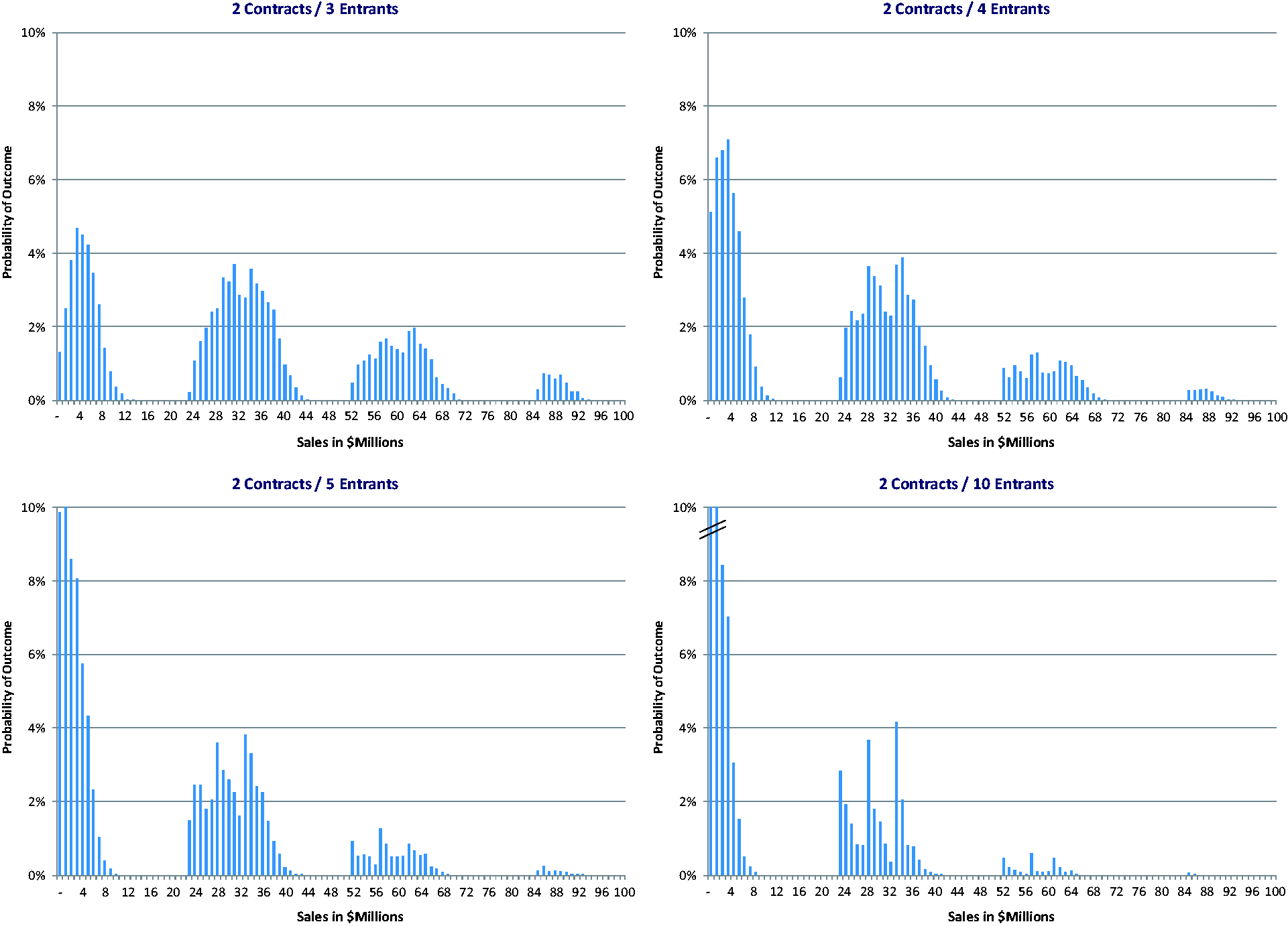
At this point, we can clearly see that the yes/no nature of wholesaler bidding causes the values to fall into one of four groups (in the 10-entrant chart, the rightmost/high-value group is difficult to see because the probability of achieving that sales level is very small). Technically, the four distinct curves in each chart are described as quadri-modal distributions but, from a practical standpoint, it is easier to think of each as describing the range of minor outcomes surrounding one of four major outcomes where a major outcome is defined as winning a Big 3 primary contract. The leftmost (lowest value) cluster is associated with no wins of this type while the rightmost (highest value) cluster is associated with winning four of these contracts.
Of interest, the market retains its four-curve shape regardless of the number of entrants but the level of competition has a pronounced impact on revenue prospects. For example, when there are three entrants, the odds of a supplier not being awarded any contracts are essentially zero. However, when there are 10 entrants, the probability of capturing no business rises to 6.5%, a rather daunting prospect considering that, to be in the bidding process at all, the generic supplier would have already incurred bioequivalence testing, ANDA approval, and other significant costs. Similarly, the probability of a windfall (i.e. winning all three Big 3 contracts along with one or more smaller pieces of business) falls quickly from 4.0% with three entrants to only 1.6% with four and 0.1% with 10 entrants. The width (i.e. range of values) of each cluster also gets narrower with more products on the market because there are fewer ways for one company to win business when competition is higher.
With primary contracts from the Big 3 wholesalers representing such a large part of the overall business, a close examination of the odds of winning one or more of these contracts is merited. Particulars will vary for each company and product but, given the economics associated with bringing a generic drug to market in the United States, it is likely that most suppliers would find that winning at least one of these contracts would represent a positive return-on-investment whereas failing to achieve this level of sales might very well be considered a loss. These probabilities are shown in Figure 3. As indicated, when three entrants are present, the odds of winning no major contracts are slightly less than 30%; a single additional entrant increases the no-win probability to 41%, and this rises to greater than 70% when there are 10 marketed products.
Probabilities of 0, 1, 2, or 3 big three wholesaler primary contract wins.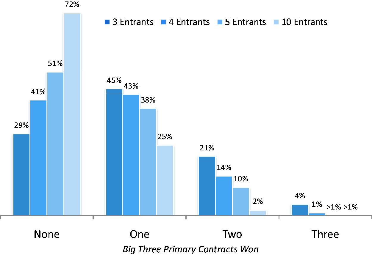
Probability distribution with 3 contracts
The results of the three contract (split 80/15/5) analysis are shown in Figure 4. In comparison to the two contract scenario, values are less likely to fall at the extreme high or low ends. The reasons for this are (a) with more available contracts, each entrant has more opportunities to win; (b) with the business parceled out in smaller amounts, the probability of outsized wins (e.g. capturing all three Big 3 primary contracts) is also reduced. In short, both risks and rewards are reduced when wholesalers issue more contracts. Also, while the four-cluster shape is retained with three contracts, the boundaries of the clusters move closer together. This follows from the fact that, with each contract added, business is awarded in smaller increments, and the market moves a little closer to satisfying the criteria for continuous variable modeling.
Probability-based generic drug sales forecast with three wholesaler contracts.
Note that the probability of winning a primary or secondary contract does not change when a third contract is available. Among other things, this means that the findings regarding Big 3 primary contract wins shown previously (Figure 3) are also applicable to the three contract scenario. This is somewhat counterintuitive but is explained by the modeling parameter that generic manufacturers will always take the best contract available (a primary over a secondary, a secondary over a tertiary, etc.). Thus, competition takes place within rather than across contract levels. As shown above, however, the availability of the third contract does affect revenue forecasts because the business is divided into a larger number of smaller pieces.
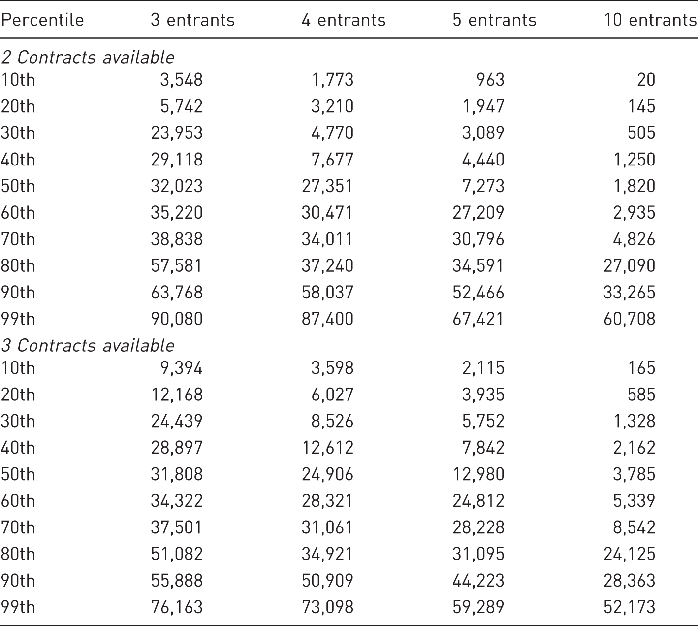
Percentile breakdown of generic drug revenues with 2 and 3 wholesaler contracts
Percentile breakout of generic drug revenues by number of wholesaler contracts and competitors
Discussion
To fully appreciate the value of MCA in this application, it may help to note that there are theoretically more than one million possible win/loss permutations with the two-contract scenario and more than one billion with the three-contract scenario. In practice, the condition that requires generic suppliers to always take the best contract available would reduce these numbers but tracking allowed permutations one by one would still be well beyond the capabilities of a standard spreadsheet model (or the patience of the spreadsheet modeler).
There are some limitations to the preceding analysis. First, the wholesaler share data on which the analysis is based are derived from the overall US pharmaceutical market and, as a result, includes brand and specialty drug distribution, which may differ somewhat from generic-only distributor share figures. Of greater importance is the fact that our model is not a perfect reflection of the environment it seeks to represent. For example, we have not accounted for the impact of price on probability of contract wins or revenues. Price is of paramount importance in actual wholesaler decision-making. In practice, optimal pricing strategy can be readily incorporated into a probability-based model but addressing it here would add an additional layer of complexity to this discussion, the primary purpose of which is to demonstrate the binary nature of the US generic market and the forecasting implications of this.
Aside from ignoring prices, the most notable difference between our model and the real world may be the model parameter that competitors have an equal chance of winning contracts. In the real world, some firms possess advantages arising from quality, reputation, service, and personal relationships between the wholesaler and the generic company, as well as other possible points of competitive differentiation. Our company’s experience, however, suggests that these factors are of modest importance; in general, once the FDA has approved the drug, generics are viewed as commodity products where price is the deciding factor and other considerations only come into play in “all other things being equal” situations.
In addition, the figures shown here are based on the results from 10,000 iterations of the MCA model, collectively known as a simulation. Because there is variability at the iteration level, there can also be variability at the simulation level, as a result of which another simulation of 10,000 iterations might return slightly different probabilities. This is more of a problem with models that have higher inherent variability and when the simulation is based on relatively few iterations. Because our choices are constricted to yes/no contract wins and the simulation consists of 10,000 iterations, the variability between the results shown here and another simulation would be very small.
Despite these limitations, we believe that both the model parameters and results are a reasonable representation of the situation facing generic drug manufacturers in the United States. Provided that the model conditions described earlier hold true, the results shown here (particularly, the percentile and sales data in Table 2) can be applied to other generic markets by scaling up or down from US$100 million. Put differently, revenue probabilities in a US$50 million market would be half the levels shown in Table 2 or twice these levels in a US$200 million market.
This analysis demonstrates that, at least from the manufacturer’s perspective, sales of generic drugs in the United States are determined by a relatively small number of wholesaler contracts that are either won or lost in totality. Furthermore, while the number of total contracts is limited, commercial success or failure will likely be dictated by the outcome of a much smaller number of large-scale contracts. As a result, the shape of the revenue distribution curve is substantially different than would be the case for a continuous variable market. Although situations with multiple binary variables are difficult to model using standard spreadsheet techniques, probability-based approaches such as MCA are well-suited for these tasks. Applied to a hypothetical generic drug market, MCA reveals the four-cluster nature of revenue distribution and the impact of competition on the probabilities associated with achieving various sales levels.
Given that the category now accounts for more than 80% of all dispensed prescriptions, generics are the pharmaceutical industry’s most widespread example of a binary market. However, the technique discussed here has application for other types of drug marketing as well. Examples include hospital pharmaceuticals, particularly in cases where a small number of trauma or children’s hospitals make up the majority of the market and sectors where group purchasing organizations play a major role in controlling access.
Footnotes
Funding
This research received no specific grant from any funding agency in the public, commercial, or not-for-profit sectors.
Conflict of interest
The author declared no potential conflicts of interest with respect to the research, authorship, and/or publication of this article.