
Abstract
In this study, indoor air humidity and temperature levels have been measured in 117 houses in Trondheim, Norway. The houses were randomly selected for each of the following types: detached one-family houses, semidetached two-family houses, row houses, and apartment buildings. The temperature and relative humidity (RH) were measured at 15-min interval over a period of 1 week. The measurements were made in bedrooms, living rooms, bathrooms, and outdoors. The internal moisture excess, which is the difference between indoor and outdoor air water vapour content, was calculated. The dataset was analysed in regard to average values of internal moisture excess and its dependency of outdoor climate. The daily variations of indoor RH, temperature, and internal moisture excess for the various types of rooms were also analysed. The typical diurnal variations of RH, temperature, and internal moisture excess are presented together with the statistical variation. The effect of influencing factors such as occupancy (area per person), type of basic ventilation of the house, type of building, time of the year, and the level of average indoor air humidity was investigated.
To get a deeper understanding of some of the factors influencing the diurnal variations of the indoor air humidity observed in the field measurements, computer simulations of the indoor air humidity were also performed. The simulations were made using the numerical software WUFI Plus.
Introduction
Knowledge of the indoor air humidity in houses is required for many purposes. High indoor air humidity and dampness in buildings may give favourable conditions to microbial processes that can be harmful to the health of the occupants of the building (Bornehag et al., 2004). Oreszczyn et al. (2005) found a clear relationship between the occurrence of mould growth in houses and the indoor air humidity. Indoor air humidity may influence on the perceived indoor air quality. Low humidity can for instance give irritation symptoms in eyes and upper airways (Wolkoff and Kjærgaard, 2007).
One of the most important input parameters when doing a hygrothermal analysis of the building envelope using simulation models is knowledge about typical levels of indoor air humidity. For many purposes, knowledge of the average indoor air humidity over a certain time period (week, month, year) is sufficient and that is also what has been documented and reported in most large-scale measurements of indoor air humidity levels in houses. In some cases however the knowledge of typical daily variations of the indoor air humidity is needed, for instance, when assessing the risk for internal surface condensation or when assessing the moisture buffer effect of the hygroscopic materials in a room (Rode and Grau, 2008). The moisture storage capacity of the interior building surfaces and furnishings may damp the diurnal changes in indoor air humidity, which has been the focus of many previous investigations (e.g., Derluyn et al., 2007; Simonson et al., 2004a, 2004b; Vereecken et al., 2011). We also register that instantaneous measurements of indoor air humidity are often made without realising that one single measurement value may be rather uninteresting considering the large variation throughout the day and week.
A common way of expressing the indoor air humidity load is by the internal moisture excess, defined as follows:

where Δv = internal moisture excess (g/m3); vi = indoor air water vapour content (g/m3); ve = outdoor air water vapour content (g/m3). The internal moisture excess is often used instead of relative humidity (RH) when the RH is not controlled but allowed to undergo wide variations due to several factors such as weather conditions, building characteristics, moisture generation, and ventilation. Another often used term for internal moisture excess is moisture supply.
It is generally considered that the internal moisture excess tends to be relatively constant in a house during the colder part of the heating season (outdoor temperature < ~0°C), while it decreases when the outdoor temperature increases. In the standard EN ISO 13788 (2001), this is expressed as the internal moisture excess being constant for outdoor temperatures below 0°C, while the internal moisture excess decreases linearly to 0 g/m3 at outdoor temperatures of 20°C, see example in Figure 3. Above 20°C, the internal moisture excess is 0 g/m3. EN ISO 13788 defines five standard humidity classes to be used as design values in hygrothermal calculations. For houses, two classes are applied: class 3: Δv = 4–6 g/m3 for dwellings with low occupancy (large area per person) and class 4: Δv = 6–8 g/m3 for dwellings with high occupancy (little area per person). The values apply when outdoor temperature is below 0°C. The standard recommends to use the upper limit value for each class unless the designer can demonstrate the conditions are less severe. According to Kalamees et al. (2006), a more correct representation of the design curves would be a constant internal moisture excess below ~+5°C and a linear decrease down to a constant value at ~+15°C and higher temperatures.
Internal moisture excess in houses has been investigated in many earlier field studies. Tolstoy (1993) measured the internal moisture excess during winter in about 1500 houses in Sweden. The internal moisture excess for single-family houses was between 2 and 5 g/m3, with an average of 3.6 g/m3. For multi-family dwellings, the internal moisture excess was between 1.5 and 4 g/m3, with an average of 2.9 g/m3. Several other field studies have been performed; a summary is given in the study by Kalamees (2006). According to Kalamees (2006), most of the studies yield average internal moisture excess during winter between ~2 and 3 g/m3 for living rooms. The variation between different houses are, on the other hand, quite large, meaning that design values for hygrothermal calculations should be selected somewhat higher than the average values.
The International Energy Agency Annex 24 (Sanders, 1996) has recommended the use of the 10% critical level for climate loads when doing a hygrothermal simulation of the external envelope. This means an internal moisture excess higher than the critical level should not appear in more than 10% of the cases. Kalamees et al. (2006) did full-year measurements in houses with low/medium occupancy (average 42 m2/person) and calculated that the 10% critical level was close to 4 g/m3 during the cold period (Tout≤+5°C) and close to 1.5 g/m3 during the warm period (Tout≥+15°C). The average values were 1.8 and 0.5 g/m3 for the cold and warm period, respectively.
While there are many studies that investigate the mean indoor air humidity in houses over a prolonged period of time, the number of studies that investigate the daily variations is fewer. Most studies that include daily variations involve measurements in only a few number of houses, few types of houses, and few types of rooms, that is, the data are not representative for a national housing stock as a whole. Mihalka and Matiasovsky (2007) report daily variation of vapour production (in kilogram per hour) measured in the central hall in four identical flats in an apartment building in Slovakia. Holm et al. (2005) made measurements of RH in the living room in 11 houses of various types in Germany, showing examples of typical daily and weekly variations. Holm et al. (2005) reported that the daily fluctuations were around the same bandwidth during both summer and winter. The fluctuations ranged between ±6% and 20% RH. Winterly daily fluctuations of RH often depend on fluctuations in the temperature. The highest fluctuations were found for low room volumes and rooms with a low wood percentage in envelope (i.e., low moisture buffer capacity).
The English Warm Front project measured daily fluctuations of internal moisture excess for living rooms and bedrooms in 1600 low-income households (Ridley et al., 2007). The general findings in the study by Ridley et al. (2007) were that the internal moisture excess in the living rooms increases in the morning when people get up from bed, that there were peaks at noon if people were at home, and that there were a peak in the evening when people were using the room after dinner. For the bedrooms, the daily variations were smaller than in the living rooms, but following the same trend, a small peak in the morning and a larger peak in the late evening were observed. The decrease of internal moisture excess during the night was generally slower in the bedrooms than in the living rooms. While Ridley et al. (2007) found almost no daily variation of RH in the living rooms, Holm et al. (2005) found the same daily trend for RH as Ridley et al. (2007) found for internal moisture excess.
Zhang and Yoshino (2010) analysed the indoor humidity levels in living rooms and bedrooms for 76 houses in nine regions of China. The average diurnal fluctuations of indoor RH were above 10% for all the nine regions and above 20% for some regions. The diurnal fluctuations were generally higher during summer than in winter.
Kalamees (2006) documented the daily variations of indoor climate in bedrooms and living rooms in 46 lightweight timber-frame detached houses in Finland. Balanced ventilation showed significantly lower daily variation of RH and internal moisture excess than exhaust ventilation. Rooms with hygroscopic indoor surface materials had significantly lower daily variations of RH and internal moisture excess than rooms with non-hygroscopic indoor surfaces.
Korpi et al. (2008) investigated the daily variations of indoor RH, temperature, and absolute humidity in the master bedroom in 69 heavyweight detached houses in Finland. There was relatively little variation between summer and winter variations. Different types of heavyweight exterior walls had little influences on the indoor air humidity. For timber-frame houses, a higher variation of humidity and temperature than that in heavyweight houses is reported.
The measurements presented in this article have been a part of the study ‘Prevention of Atopy Among Children in Trondheim’ (Jenssen et al., 2001). The analysis of the measurements has been a part of the ongoing SINTEF strategic institute project ‘Climate Adapted Buildings’. The dataset has previously been analysed in regard to mean internal moisture excess and its dependency of outdoor climate in the study by Jenssen et al. (2002) and Geving et al. (2008) and with regard to diurnal variations in the study by Geving and Holme (2009).
Method
Field measurements
Indoor air humidity levels have been measured for a week during the heating season in 117 houses in Trondheim, Norway. Thirty-two of those houses are only included in parts of the analysis presented in this study (Figures 1–3), due to partly incomplete datasets for the needed analysis. The measurements in the 32 houses are previously presented in the study by Jenssen et al. (2002). The main analysis is, therefore, conducted on the remaining 85 houses. It should be noted that the distributions (percentages) given in this chapter refer to the 85 houses. The houses were selected for each of the four following building types: detached one-family houses (41%), semidetached two- or four-family houses (28%), undetached (chained) houses (13%), and apartment buildings (18%). Most of the houses in Norway (except for apartment buildings) are lightweight timber-frame houses and so was the case also in this study.
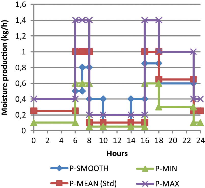
Diurnal variation for the chosen moisture production profiles.
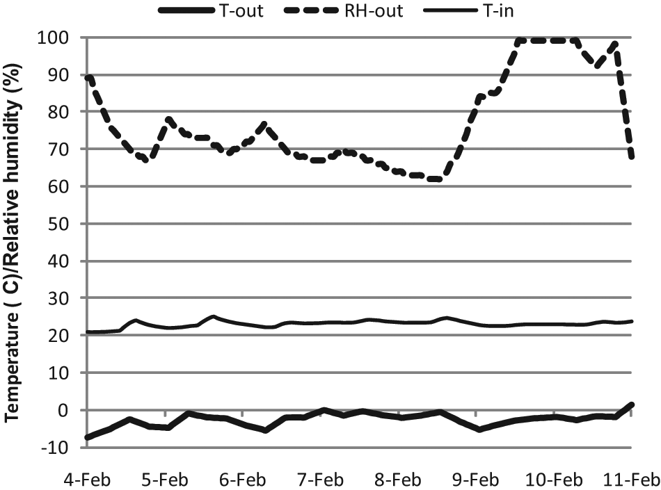
Outdoor temperature and RH and calculated indoor temperature during the chosen week (4 February 01:00 a.m. to 10 February 24:00 p.m.).
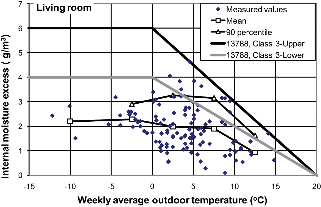
Internal moisture excess for various outdoor temperatures in the living rooms. The dots represent the weekly mean value for one particular house (N = 117).
In each house, measurements were made in a bedroom, the main living room, and the most used bathroom. The bedroom was selected to be the bedroom where the child included in the ‘Prevention of Atopy’ study slept and that would typically be the master/parent bedroom since the children typically was under 1-year old. However, some children have probably been sleeping alone without their parents in a children’s bedroom.
The year of construction had the following distribution: before 1961 (34%), 1961–1983 (37%), and after 1983 (29%). The mean heated floor area of the houses was 127 m2 (standard deviation (SD) = 89 m2). Non-heated areas such as cold cellars are not included in this floor area. Most of the studied rooms had the possibility of opening the windows for airing purposes. The houses had all types of basic ventilation: no ventilation (8%), natural ventilation (55%), mechanical exhaust ventilation (30%), and balanced ventilation (7%). ‘No ventilation’ means that there was not installed any airing inlets/outlets in walls or window frames.
The 85 houses were selected through the following procedure: Parents of the children who were included in the ‘Prevention of Atopy’ study were asked for permission to perform inspection of their houses until enough participants had accepted. There were 200 participants in this home inspection study, but RH and temperature were measured in only 85 of these 200 houses. This means that the houses were ‘randomly’ selected among a population (with small children in the house) that had accepted to participate in the ‘Prevention of Atopy’ study. The other 32 houses were selected through the following procedure: A total of 300 buildings in Trondheim were randomly selected for each of the four building types mentioned earlier. For each building, one family was selected to receive a questionnaire. The response rate was 35%. Eight or nine buildings of each type were randomly selected for home inspections and measurements.
The temperature and RH were measured at 15-min interval over a period of 7 days. Small logging units were used (Tiny tag, TGU 1500, Intab). The loggers were positioned away from windows, heating units, direct sunlight, or outer door. The loggers were placed between 1.5 and 2.0 m above the floor level. The accuracy of the loggers were ±3% RH and ±0.5°C. Hourly data for outdoor RH were retrieved from an automatic weather station located in Trondheim operated by the Norwegian Meteorological Institute, with an accuracy of ±2% RH and ±0.5°C. The internal moisture excess (Δv) was calculated on an hourly basis. The measurements were made during the period May to July 2003, September 2003 to June 2004, and September to December 2004. In 45 of the houses, the weekly average outdoor temperature was below 5°C during the measurements, and for the last 42 houses, the outdoor temperature was between 5°C and 15°C.
Simulations
To get a deeper understanding of some of the factors influencing the diurnal variations of the indoor air humidity observed in the field measurements, computer simulations of the indoor air humidity were performed. The simulations were made using the numerical software WUFI Plus (Künzel et al., 2003). WUFI Plus is a whole building simulation model that solves the transient internal climatic conditions, by combining an energetic whole building simulation with a hygrothermal component model for the envelope structures. It takes into account the main hygrothermal effects such as vapour diffusion and capillary transport through the envelopes, vapour absorption/desorption of the internal surfaces, internal moisture sources, and sinks due to moisture production and ventilation.
The field measurements presented earlier represents residential buildings in Trondheim, Norway, with varying age but mostly small houses such as detached single-family houses or semidetached two- or four-family houses. In the following simulations, the input data were chosen to be as close as possible to the ‘average’ house in the field measurements. The house was modelled as a one-floor building with floor on the ground and a flat compact lightweight roof, with a heated floor area of 120 m2 (8 m × 15 m) and a floor height of 2.5 m. It was chosen to simplify the simulations by using a one-zone model, but including 28-m internal walls as extra absorption/desorption surfaces. That is, the internal walls give a total of 2 × 28 m × 2.5 m = 140 m2 surface area, while the roof and external walls totally give 235 m2 exposed surfaces to the internal air (the floor is defined with negligible moisture buffer effect).
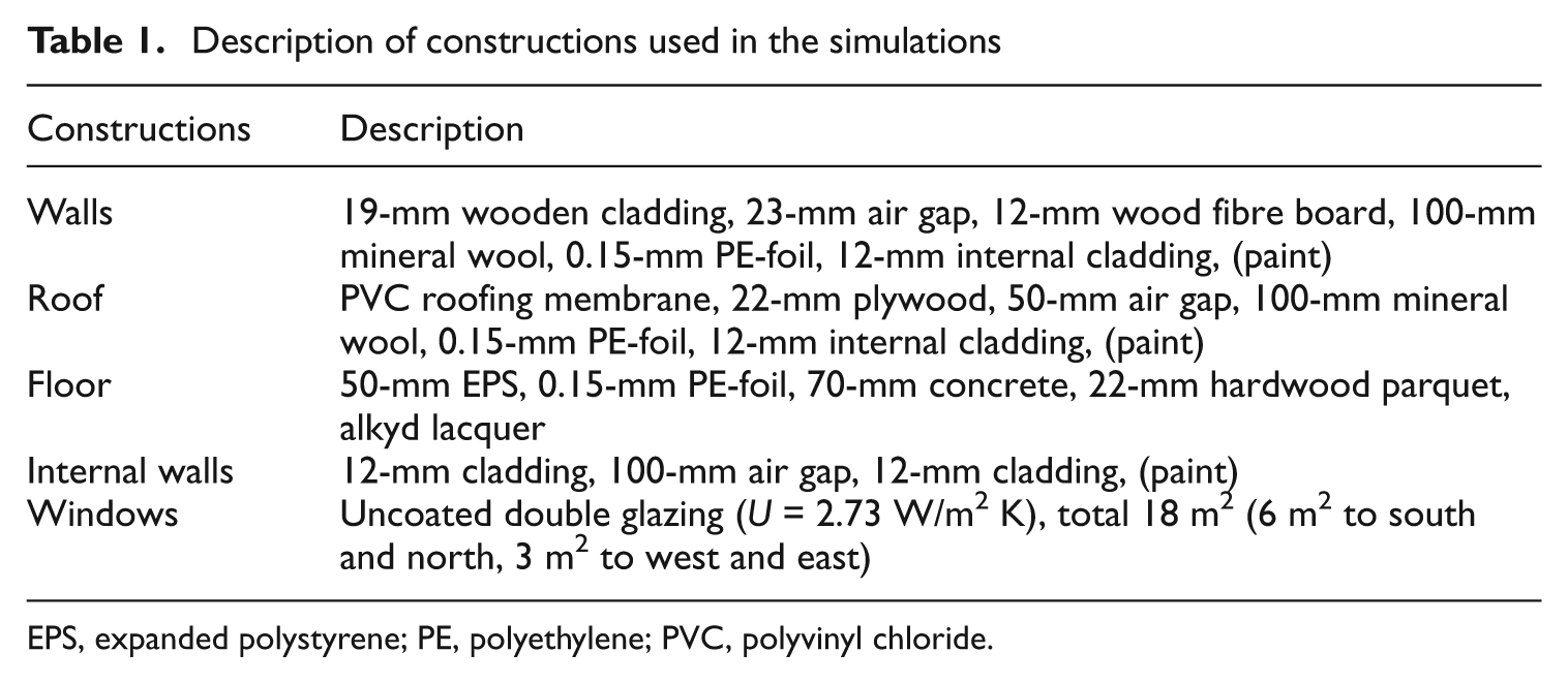
The envelope structures were typically chosen to be not too well insulated, typically like a Norwegian house from the 1970s, see description in Table 1. The roof and the external wall structures had a vapour barrier behind the internal cladding, so only the cladding would give a moisture buffer effect. The standard internal cladding used was 12-mm gypsum board with acryl-latex paint (sd,paint = 0.3 m), but parametric variations were performed with spruce cladding, both untreated and treated with alkyd paint (sd,paint = 1.0 m). In addition, a case was simulated with an aluminium cladding (sd,cladding = 50 m) on all surfaces (except the floor) to simulate the extreme case with hardly any absorbing surfaces at all. The floor surface was a hardwood parquet with a rather vapour tight lacquer (sd,lacquer = 5.0 m), so this would also not give any moisture buffer effect. The moisture buffer effect of furniture, bookshelves, and so on was however not included in the simulations, since WUFI Plus does not have that option.
Description of constructions used in the simulations
EPS, expanded polystyrene; PE, polyethylene; PVC, polyvinyl chloride.
The material parameters used in the simulations were taken from the material database of the programme. The materials influencing the most on the internal air humidity are the internal cladding and the paint. The water vapour permeability and the so-called moisture capacity (slope of the sorption curve) are important parameters for moisture buffering. Within the level of indoor air humidity occurring during these simulations (~15–40% RH), the vapour resistance factor and moisture capacity are µ = 83 and ξ = 0.25 kg/kg (spruce) and µ = 8 and ξ = 0.0042 kg/kg (gypsum board), respectively.
The definitions of the total daily moisture production and the variation over the day are, of course, crucial for the results. The field measurements did not supply estimates of the moisture production, so it was chosen to use Swedish estimates of average moisture production based on measurements from 1200 houses (Tolstoy, 1993). The average moisture production for single-family houses was found to be Gmean = 9.8 kg/day, and this value was used as the standard value. In addition, parametric studies included both a higher and a lower total moisture production: Gmin = 5 kg/day and Gmax = 15 kg/day. Gmin and Gmax represent approximately 10th and 90th percentiles, respectively, on the distribution curves of the measurements made by Tolstoy (1993).
The variation of the moisture production over the day is however the most uncertain parameter. It was decided to consider the living room in a family where both adults are working ordinary hours (8 a.m. to 16 p.m.). Since the simulations are based on a single-zone model, we assume that the whole house is a living room, any moisture transport from other rooms, such as bathroom, bedroom, and so on, therefore has to be modelled into the daily variation of the moisture production. Four different moisture production profiles were tested as shown in Figure 1, the profile P-MEAN (based on Gmean = 9 and 8 kg/day) being used as the standard profile. While the profiles P-MEAN, P-MIN (Gmin = 5 kg/day), and P-MAX (Gmax = 15 kg/day) basically follow the same diurnal variation, another daily profile with a more smoothed variation was also tested: P-SMOOTH (Gmean = 9 and 8 kg/day).
The chosen air change rate is based on measurements made by Øie et al. (1998) of 344 residences in Oslo in Norway. The average air change rate was found to be ~0.55 1/h, and this was used as the standard value in the simulations. It should be noted that Øie et al. (1998) compared this with measurements from the other Nordic countries and found the Norwegian air change rate to be higher than in the other countries. This was explained by different inhabitant behaviour. In the parametric study, two other air change rates of 0.35 and 0.8 1/h were also included. They represent approximately 20th and 80th percentiles, respectively, on the distribution curves of the measurements made by Øie et al. (1998).
It was chosen to simulate 1 week of winter conditions using the climatic file of Værnes in WUFI Plus, which is located only 30 km from Trondheim. The chosen week was in February, because there were relatively small changes in the outdoor temperature that week (weekly mean = −2.5°C). To be certain, the indoor surfaces were little influenced by the initial temperature and moisture conditions, and the previous 4 weeks were also included in the simulations. An internal convective heating of 5 kW (for cases 8 and 9, 4.5 and 5.7 kW were used, respectively) was chosen, allowing the indoor temperature to vary between 21°C and 25°C for the considered week. Figure 2 shows the indoor (calculated) temperature and outdoor temperature and RH during the chosen week.
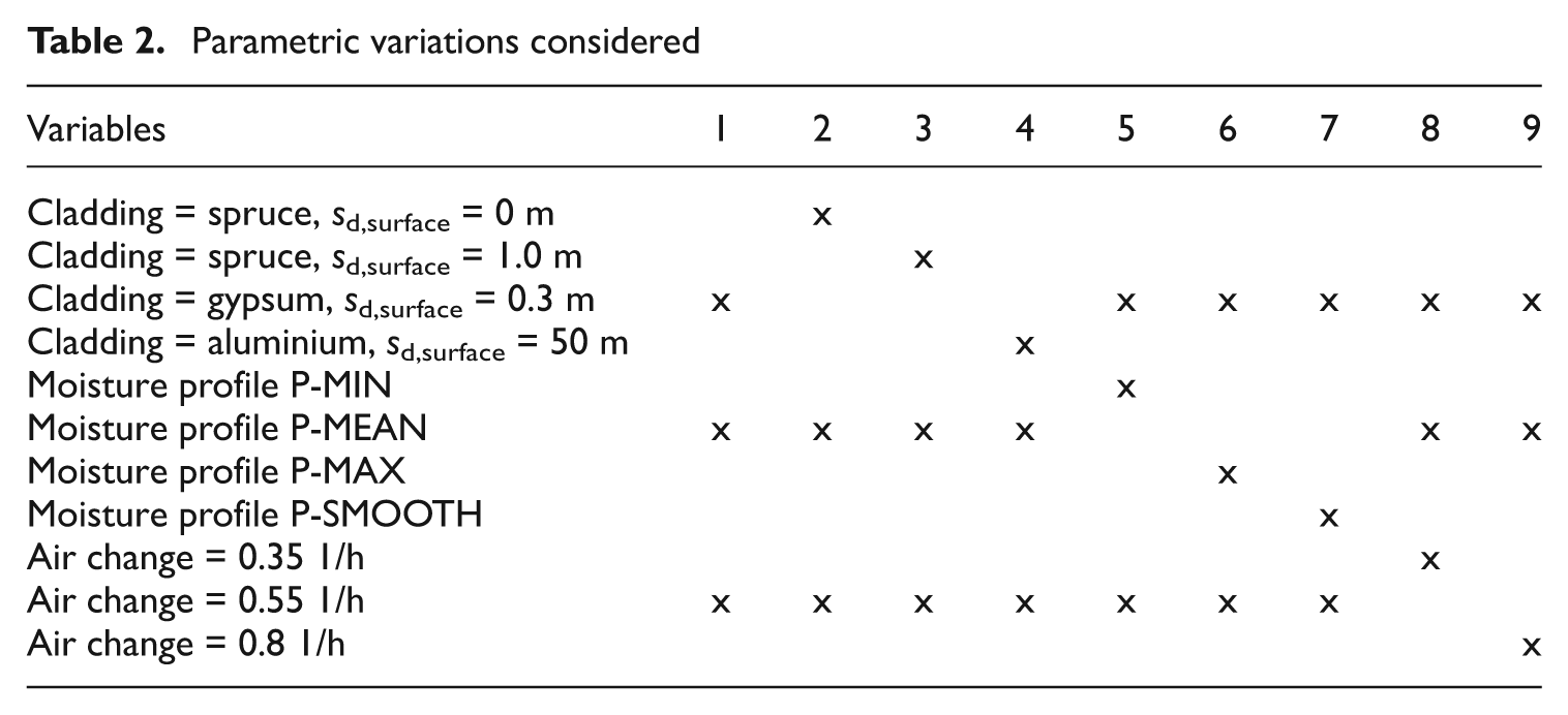
A total of nine simulations were performed. The different simulation cases are described in Table 2.
Parametric variations considered
Results
Measured mean values
Mean values (mean of 1 week) of indoor climate parameters are given in Table 3. Since it is shown that these parameters varies over the year, that is, they are dependent of the outdoor temperature, the values are divided into two groups for weekly mean outdoor temperatures below and above 5°C. A detailed visualisation of the dependence is given in Figures 3–5. All analyses are made on the basis of weekly means of the internal moisture excess and outdoor temperature from each house. The 90th percentile (i.e., 10% critical level) of internal moisture excess has been calculated together with the mean values (when enough valid N) for intervals of the outdoor temperature. In Figures 3–5, the EN ISO 13788 internal humidity class 3 (dwellings with low occupancy) limit curves are given for comparison.
Mean values of indoor RH, temperature, and internal moisture excess
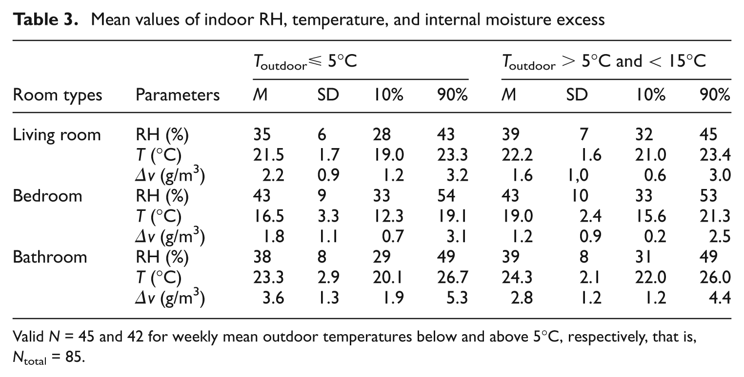
Valid N = 45 and 42 for weekly mean outdoor temperatures below and above 5°C, respectively, that is, Ntotal = 85.
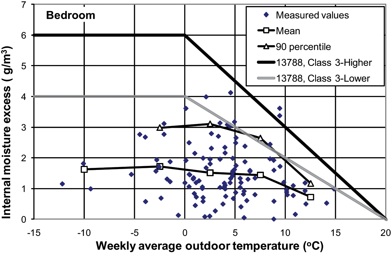
Internal moisture excess for various outdoor temperatures in the bedrooms. The dots represent the weekly mean value for one particular house (N = 117).
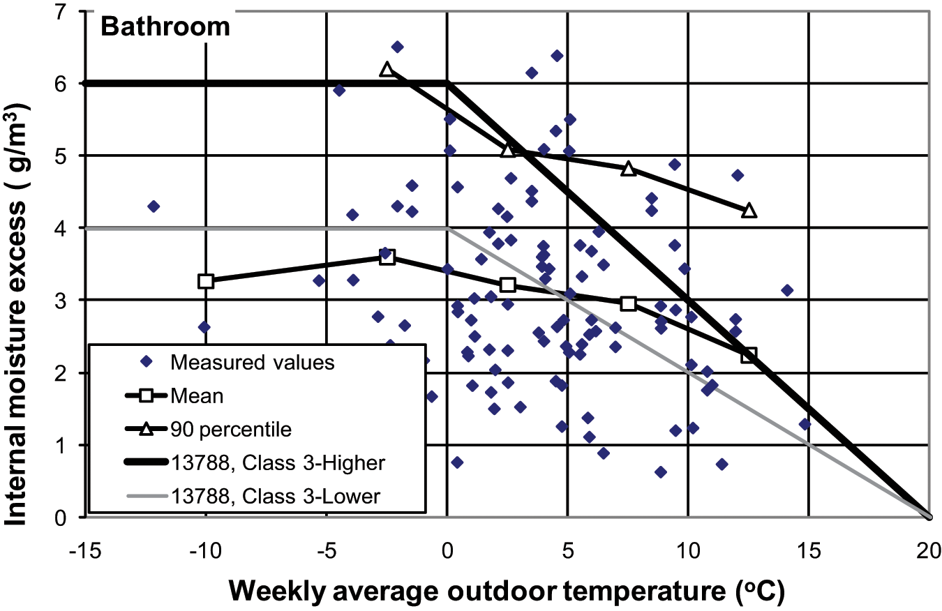
Internal moisture excess for various outdoor temperatures in the bathrooms. The dots represent the weekly mean value for one particular house (N = 117).
We find from Table 3 and Figures 3–5 that the internal moisture excess is relatively constant during the winter when the outdoor temperature is less than approximately an outdoor temperature of +5°C but decreases for higher outdoor temperatures. A significantly higher (p < 0.03, paired samples t-test) internal moisture excess for outdoor temperatures below +5°C compared with internal moisture excess for outdoor temperatures above +5°C was found for the living rooms and the bathrooms. For bedrooms, this difference was not significant (p = 0.08).
The analysis showed that the mean weekly internal moisture excess in bathrooms were significantly higher (p < 0.05, analysis of variance (ANOVA) test) than all other room types for all outdoor temperatures (below and above +5°C). The internal moisture excess in living rooms was significantly higher than in the bedrooms for outdoor temperatures below +5°C. Due to the strong dependence of room type, the rest of the analysis is made for each room type separately.
The effect of level of occupancy, building year, and basic ventilation system of the house is given in Table 4. An effect of level of occupancy was found for living rooms. The mean weekly internal moisture excess was significantly lower (p < 0.05, ANOVA test) for low occupancy (<0.02 person/m2) compared with higher occupancy (>0.02 person/m2). There was however no significant difference between a high level of occupancy (>0.033 person/m2) and a medium level of occupancy (0.02–0.033 person/m2). For the bedrooms, we also see a tendency to higher internal moisture excess for higher occupancy; however, this effect was not significant. For bathrooms, the internal moisture excess was significantly lower (p < 0.05, ANOVA test) for low occupancy (<0.02 person/m2) compared with medium occupancy (0.02–0.033 person/m2).
Mean internal moisture excess during the colder part of the heating season (outdoor temperature < +5°C) for various degrees of occupancy (heated area per person), various periods of building year, and various types of basic ventilation
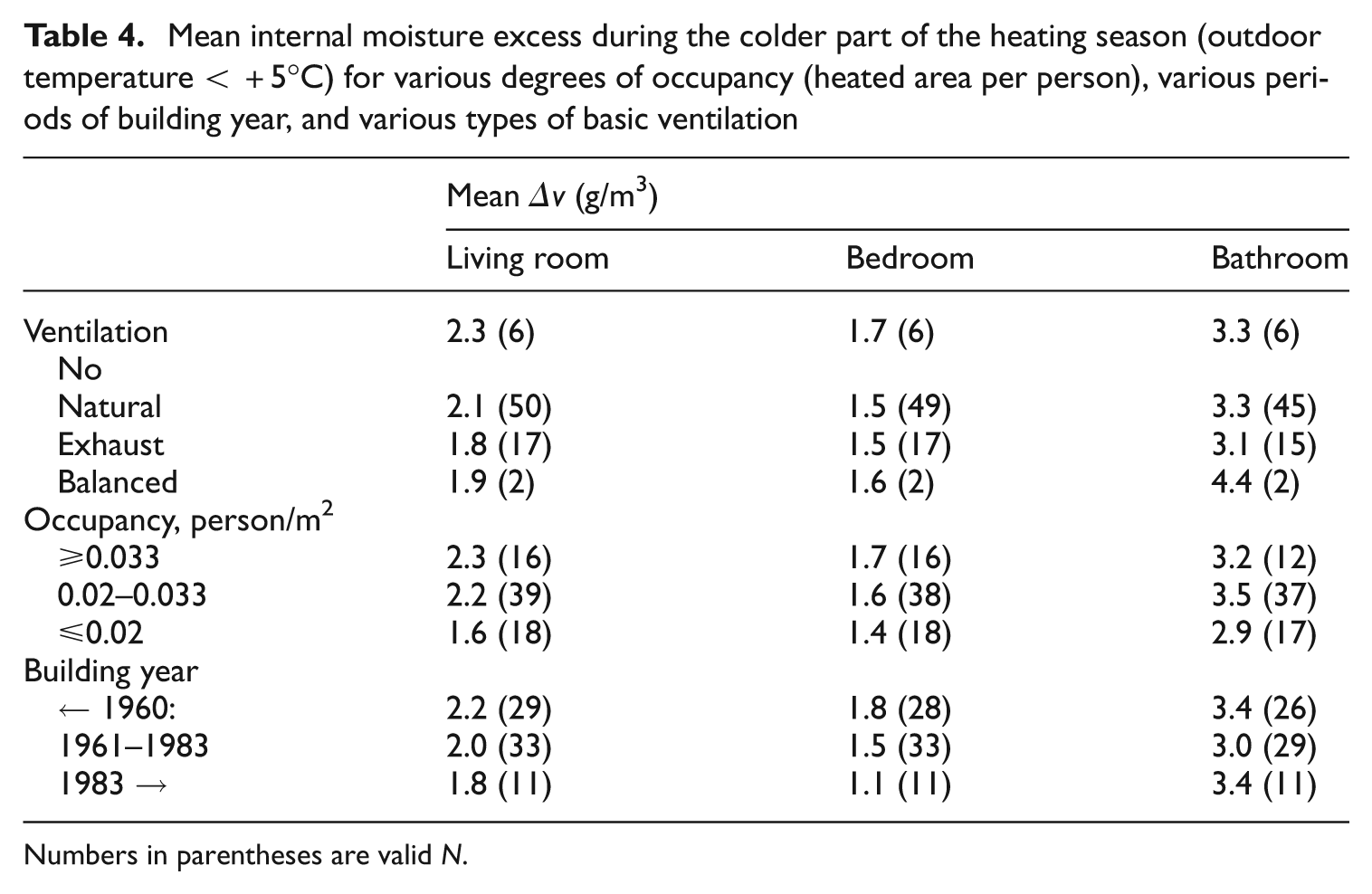
Numbers in parentheses are valid N.
Table 4 shows that there is a tendency for the living rooms and bedrooms to have a higher internal moisture excess when older the house is. This difference was however not significant (p >> 0.05, ANOVA test). For the living rooms, we find a small tendency to a decrease of the internal moisture excess as the ventilation system improves from no ventilation to natural and mechanical ventilation. This difference was however not significant (p >> 0.05, ANOVA test). The effect of a single-exhaust fan in the bathroom was not investigated. There was no significant difference found (p >> 0.05, ANOVA test) in mean weekly internal moisture excess between the various building types (one-family houses, two- or four-family houses, chained houses, and apartments).
Measured diurnal variations
The daily variations of the indoor climate parameters are given in Table 5. For each house and each room, the mean daily variation (daily variation is defined as the difference between maximum and minimum hourly value during the day) was calculated based on seven daily values during the week. Based on these values, the mean and SD is calculated for the group of 85 houses.
Mean daily variations of indoor RH, temperature, and internal moisture excess (valid N = 85)
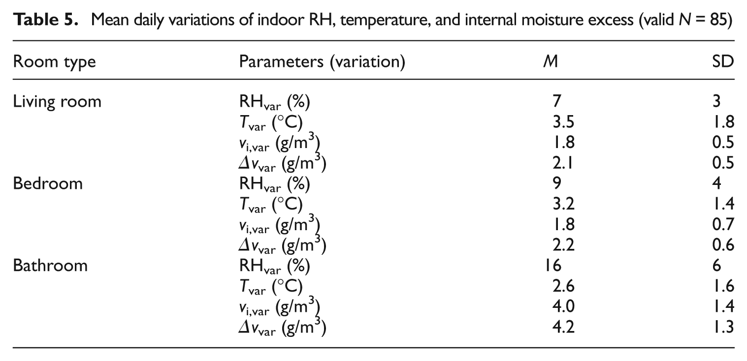
It is interesting to see from Table 5 that the mean daily variation of vi (vi,var) is slightly less than the mean daily variation of Δv (Δvvar) for all the room types. If ve was constant during the day, these two values should be the same, but since ve is varying during the day, this is not the case. The significance of this was however not investigated any further.
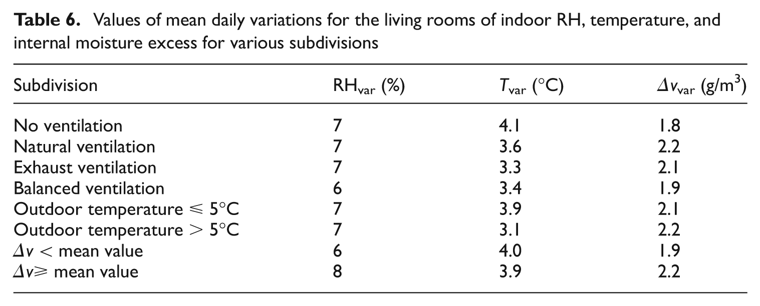
It was investigated whether the mean daily variation depended on the time of the year. When comparing the groups of houses with weekly mean outdoor temperatures below and above 5°C, only small differences were found. The effect of the type of ventilation on the mean daily variation was also investigated. The differences were rather small (no significant differences were found). When comparing subdivisions for houses with internal moisture excess below and above the mean value, we found a significantly higher Δvvar when the internal moisture excess was higher than the mean value compared with when the internal moisture excess was lower than the mean value. As an example, the effect of these subdivisions is shown in Table 6 for the living rooms only.
Values of mean daily variations for the living rooms of indoor RH, temperature, and internal moisture excess for various subdivisions
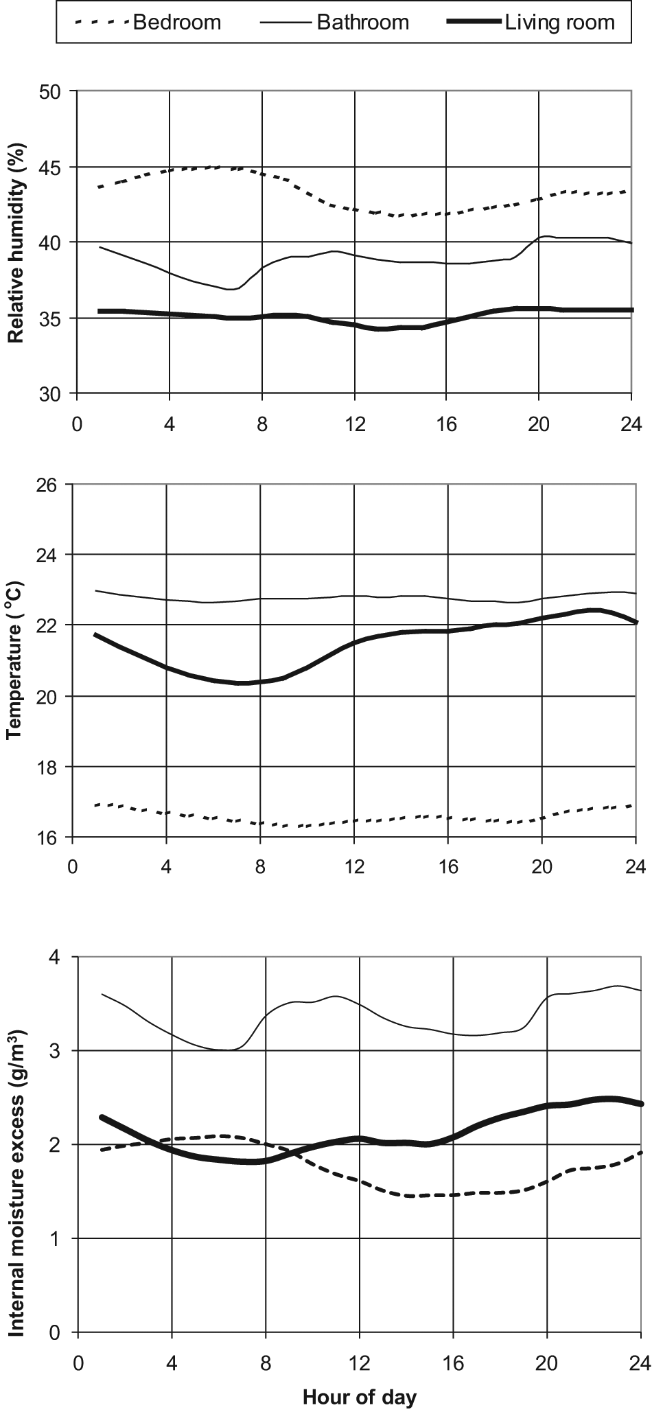
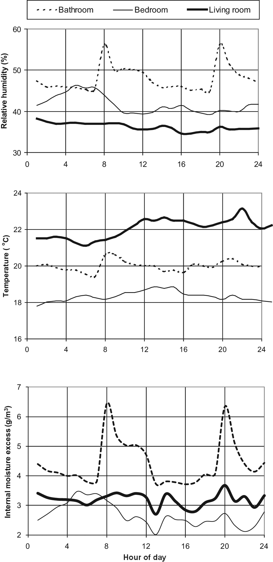
The typical variation of indoor air temperature, RH, and internal moisture excess throughout the day is shown in Figures 6 and 7. For every house and for every hour of the day (1 a.m. to 24 p.m.), a mean value is calculated for a particular time of hour based on the seven values throughout the week. Based on these mean hourly values from all 85 houses, the mean value for the group of 85 houses (e.g., two groups of 45 and 42 houses) is calculated for every hour of the day.
Variation of RH, temperature, and internal moisture excess throughout the day during winter (outdoor temperature < 5°C). Mean values for 43 of the 85 houses are based on 7 days of measurement for each house.

Variation of RH, temperature, and internal moisture excess throughout the day during spring and autumn (outdoor temperature between 5°C and 15°C). Mean values for 42 of the 85 houses are based on 7 days of measurement for each house.
Since the variations throughout the day shown in Figures 6 and 7 are average values based on hourly values from 7 days and 85 houses, we realise that typical peaks will be damped due to moisture production occurring at different times during the day in different houses/families. As an example of a more typical variation throughout the day, the internal moisture excess during the day is shown for 10 arbitrarily chosen houses in Figure 8. Note that the measurements were not made the same week, but the mean outdoor temperature was within the same range. Hourly means of RH, temperature, and internal moisture excess are shown in Figure 9 for one arbitrarily chosen house during one specific day.
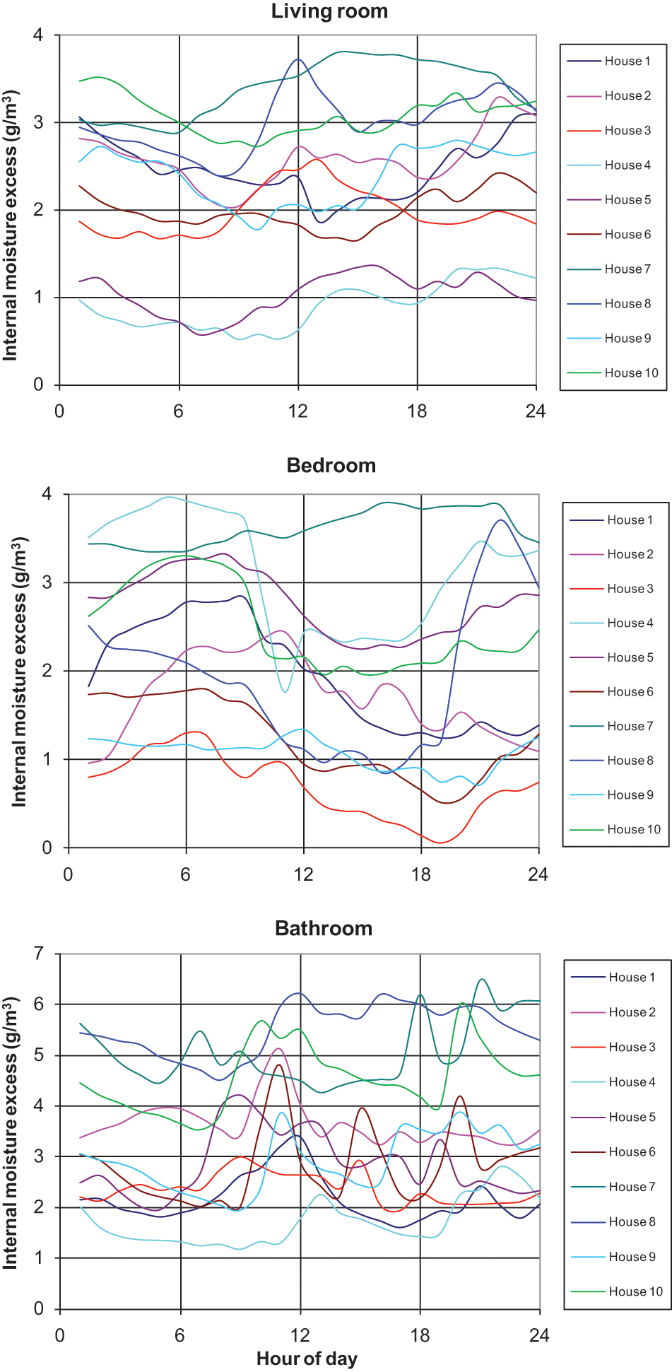
Example of variation of internal moisture excess throughout the day for 10 arbitrarily chosen houses (mean outdoor temperature was between −3°C and +1°C). Mean values are based on 7 days of measurement for each house.
Example of hourly means for RH, temperature, and internal moisture excess throughout the day measured for one specific house (no. 20973) during one specific day (daily mean outdoor temperature was −0.9°C).
Measured weekly variations
When calculated on an hourly basis, we find that the internal moisture excess may vary considerably during the week if the outdoor air water vapour content (ve) changes rapidly. Two examples of the variation of internal moisture excess during a week are given in Figures 10 and 11. It is selected periods where the outdoor air water vapour content are changing relatively much during the week.
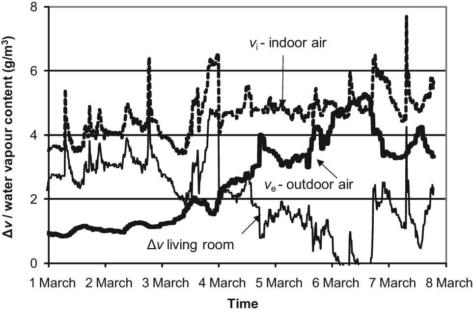
Example of the variation of the internal moisture excess in the living room throughout a week (in house no. 151), during a period where the outdoor air water vapour content is changing relatively much.
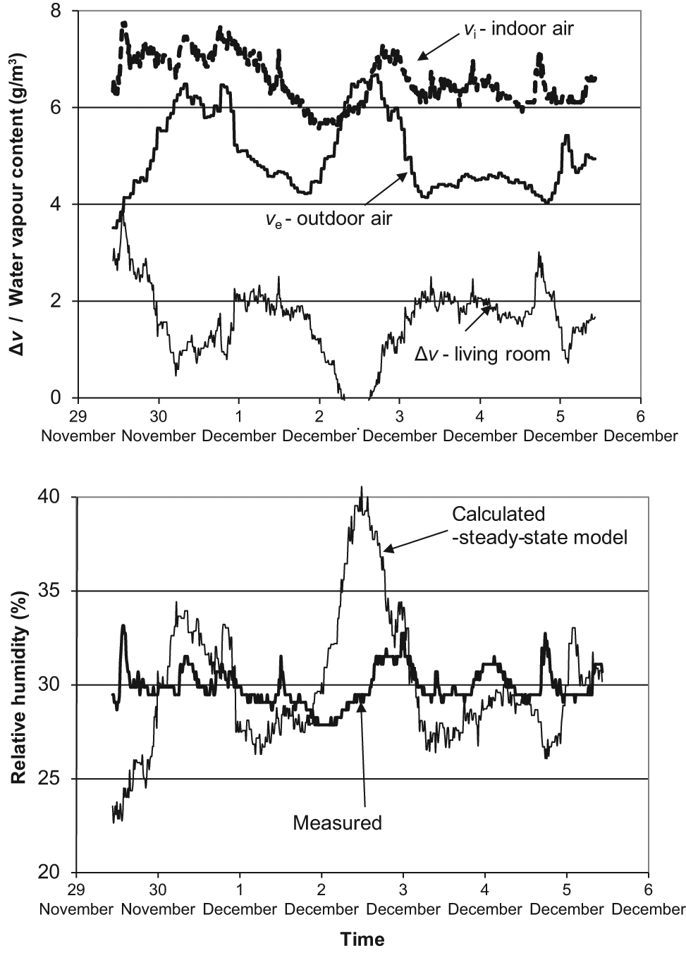
Example of the variation of the internal moisture excess and RH in the living room throughout a week (in house no. 30), during a period where the outdoor air water vapour content is changing relatively much.
Figures 10 and 11 show a decrease in the daily mean internal moisture excess over the week, as ve increases over several days. Probably due to hygroscopic surfaces, furniture, and so on, the indoor air water vapour content (vi) is not increasing at the same rate as ve, and in this way influencing the hourly and daily values of the internal moisture excess. When ve suddenly decreases, we see the opposite effect, that is, the internal moisture excess suddenly increases.
Figure 11 also shows the large discrepancy of real hourly RH and calculated RH if not including the hygroscopic inertia (moisture buffer effect) of interior surfaces. The calculated values of RH were calculated from hourly values of outdoor air water content (ve) and using the weekly mean internal moisture excess (=1.55 g/m3), that is, RH = (vi/vi,sat)100, vi = ve+ 1.55. From this, we realise, that calculating hourly indoor RH by using mean internal moisture excess may lead to much higher fluctuations of RH than what is occurring in reality.
Simulated diurnal variations
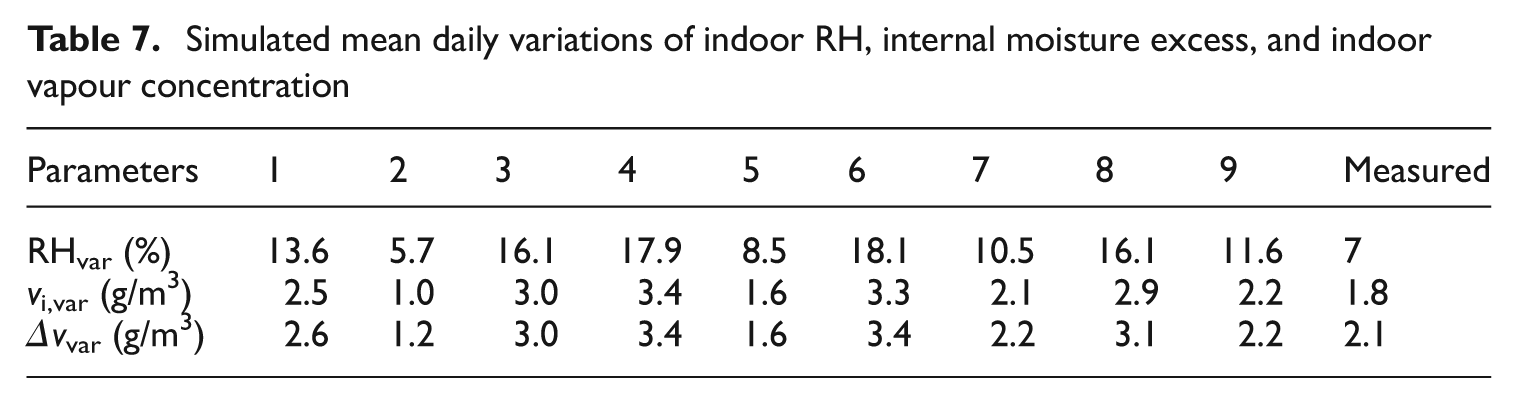
Mean daily variation of the indoor climate humidity parameters are given in Table 7, together with the measured values given in Table 5 for the living room. Daily variation is also defined as the difference between the maximum and minimum hourly value during the day, and the mean daily variation is calculated from seven daily values from the considered week. We see from Table 7 that the calculated values (especially for RH) are much higher than the measured, with an exception of cases 2 (untreated spruce), 5 (Gmin = 5 kg/day), and partly 7 (‘smoothed’ moisture profile). The case with untreated spruce actually has lower daily variation than measured. It should be noted that it is a relatively small difference in the daily variation between the case with aluminium cladding and wooden cladding with alkyd paint.
Simulated mean daily variations of indoor RH, internal moisture excess, and indoor vapour concentration
The mean weekly values of calculated internal moisture excess are between 2.2 and 2.5 g/m3 for the cases with a moisture production of 9.8 kg/day and an air change rate of 0.55 1/h, while the measured value for living rooms during winter conditions was 2.2 g/m3 as shown in Table 3. This indicates that the chosen combination of total moisture production, air change rate, and building volume is reasonable, that is, to represent the ‘average’ house of the field measurements.
In Figures 12–14, the diurnal variation of RH is shown for one specific day for the various simulation cases. Figure 12 shows the effect of various surface materials. As can be seen from Table 7, the figure also shows that untreated wooden cladding has a large moisture buffer effect, while painted gypsum board (sd,paint = 0.3 m) and painted wooden cladding (sd,paint = 1.0 m) have a much lower moisture buffer effect. An extra case (not documented further) was simulated with a more vapour open paint on the gypsum board (sd,paint = 0.15 m), giving only a slightly better moisture buffer effect than case 1 (RHvar = 11.6% instead of 13.6%). The case with untreated wooden cladding shows higher similarity with typical daily variations as can be seen in Figures 6–9 than the other types of surfaces.
Calculated indoor RH the 7. February. Effect of various surface materials.
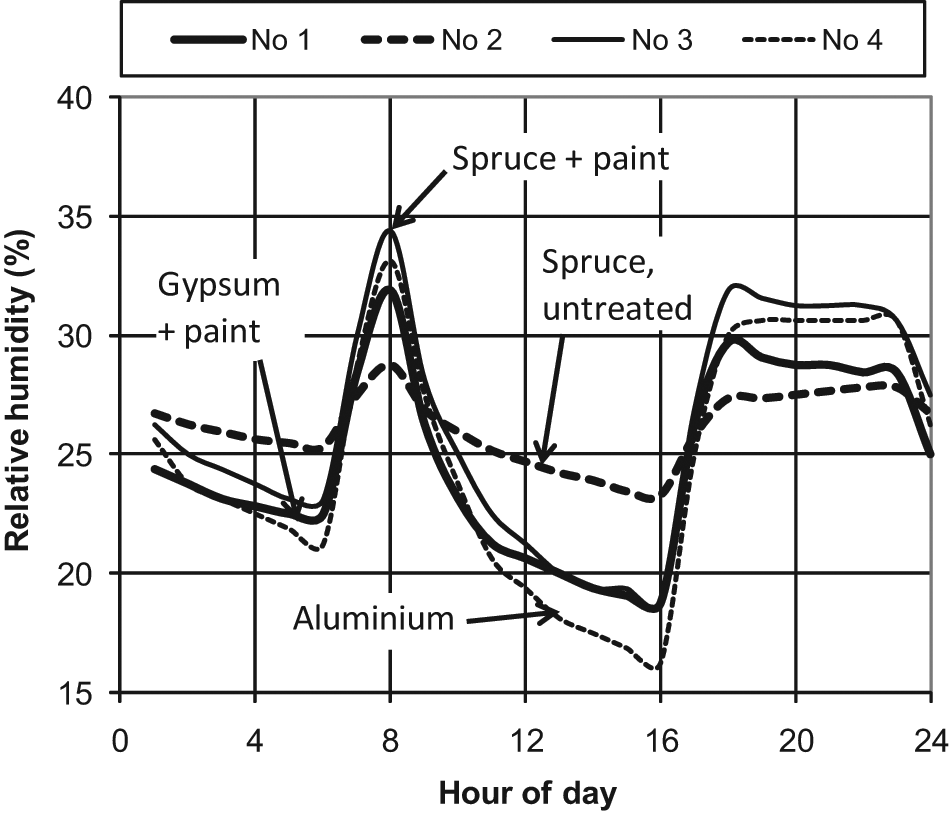
Calculated indoor RH the 7. February. Effect of various diurnal moisture profiles.
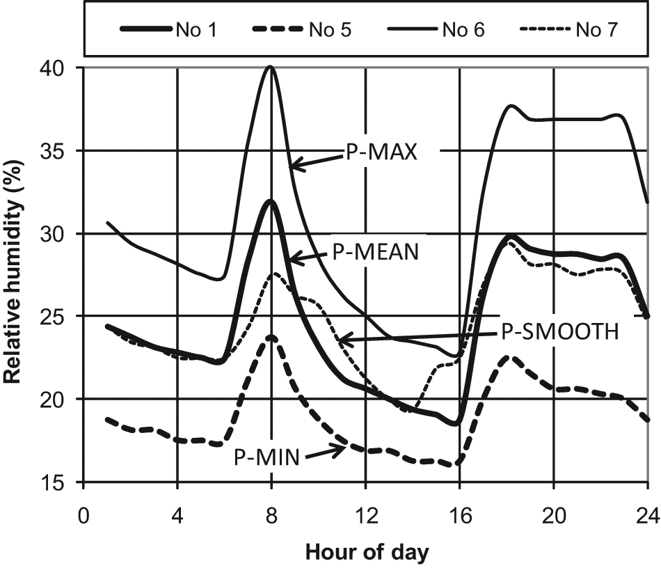
Calculated indoor RH the 7. February. Effect of various air change rates.
Figure 13 shows the effect of various moisture production profiles. As expected, we see that the higher the total daily moisture production, the higher the RH level is and the higher the variations. The ‘smoothed’ moisture profile shows higher similarity with typical daily variations as can be seen in Figures 6–9 than the other moisture profiles. Figure 14 shows the effect of various air change rates. As expected, we see that the lower the air change rate, the higher the RH level is and the higher the variations.
Discussion
Measured mean values
The measured mean internal moisture excess in the living rooms seems to be somewhat smaller than what has been measured in previous studies, being 2.1 g/m3 in this study and, for instance, 2.9 and 3.6 g/m3 for multi-family dwellings and single-family houses, respectively, in the Swedish study of Tolstoy (1993). One possible explanation to this is that it seems that the air change rate of Norwegian houses is somewhat higher than other Nordic countries, which would be natural to compare with. Øie et al. (1998) measured ventilation rates in 344 residences in Norway and generally found higher air change rates (approximately average value was 0.55 1/h) than that found in similar studies in Sweden, Denmark, and Finland. This difference was explained by Øie et al. (1998) by different inhabitant behaviours.
The results showed that the internal moisture excess is not a constant value over a year but dependent on the outdoor temperature. This effect is probably due to more ventilation (more open windows) and less moisture production (less indoor activity) during the warm period of the year. This confirms previous investigations, such as the study by Kalamees et al. (2006) and the design curves given in the standard EN ISO 13788. The deflection point of the internal moisture excess curve (i.e., when it goes from a constant value to a linear decrease as temperature increases) is not 0°C as given in EN ISO 13788 but seems, according to Figure 1, to be closer to +5°C–7°C. This confirms the findings of Kalamees et al. (2006) who claim that the deflection point should be ~+5°C.
According to EN ISO 13788, the internal moisture excess is 0 g/m3 when the outdoor temperature reaches 20°C or higher temperatures. We did not perform measurements when the outdoor temperatures were higher than +15°C, so we cannot conclude on that aspect. However, when looking on the internal moisture excess curve for bathrooms (Figure 5), it seems improbable that the internal moisture excess should reach 0 g/m3. Since windows cannot be kept open all the time even at high outdoor temperatures, it is probable that the internal moisture excess is higher than 0 g/m3 during the warm period, as was measured by Kalamees et al. (2006). Assuming that the internal moisture excess will reach a constant value of >0 g/m3 during the warm period, it seems from Figures 3 and 4 that this deflection point is closer to +15°C than +20°C as given for the design curves in EN ISO 13788. The same observation was made by Kalamees et al. (2006).
According to our measurements, it seems that the design curves given in EN ISO 13788 need to be modified to be used in hygrothermal analysis, both in regard to the shape and deflection points and in regard to the level for various occupancy and room type. The highest levels of internal moisture excess have been measured in the bathrooms, but it is probably unnecessary conservative to design the whole house according to these high levels. It is probably better to use the measurements for the living rooms as basis for the design of the whole building and do a special analysis for the bathrooms (and other similar rooms such as laundry room), if necessary. In our measurements, the bedroom values are significantly lower than the living room values. It should however be noted that the bedrooms are children’s bedrooms, and that the parent bedrooms might have higher values. Kalamees et al. (2006) report slightly higher values for bedrooms than for living rooms (0.2 g/m3 higher in average, Tout < +5°C), and this might be due to this being parents’ (two persons) bedrooms. It should however be noted that in Norway, it is rather common to sleep with open windows in the bedroom also during winter, giving a better ventilation and a lower temperature. In the study by Jenssen et al. (2002), the weekly mean temperature in 31 children’s bedrooms in Trondheim was measured to be +13.5°C ± 4.3°C.
While there was no significant effect of the ventilation system, there was a significant effect of the level of occupancy found for living rooms as shown in Table 4. From our findings and the findings of Kalamees et al. (2006), we propose the following moisture design curves based on the 10% critical level as given in Figure 15. ‘Low’ could be used for living rooms in houses with low occupancy (<0.02 person/m2) and areas where the moisture production is low (e.g., cellars), ‘Medium’ for living rooms in houses with medium/high occupancy (>0.02 person/m2) and bedrooms, and ‘High’ for bathrooms and laundry rooms. Note that these design curves apply for Norwegian conditions but may not necessarily apply to other countries.
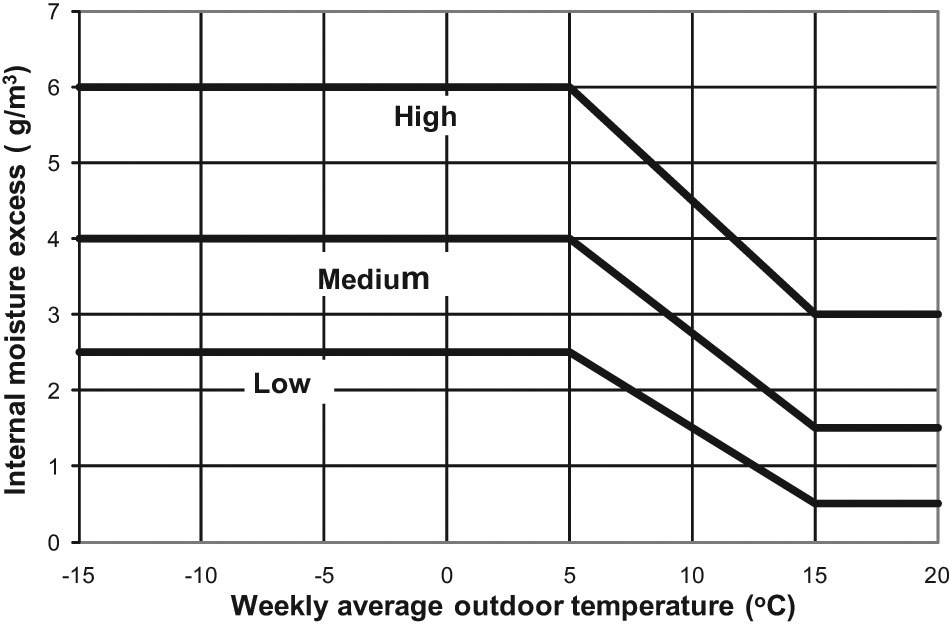
Proposed internal moisture excess design curves for houses (based on 10% critical level).
Measured diurnal variations
The daily variation of indoor air RH and the internal moisture excess in houses are generally dependent of many factors such as variation of moisture production during the day, fluctuations of indoor air temperature (e.g., by daily heating strategy, solar radiation), short-term variations of ventilation (e.g., opening windows, increasing/decreasing level of mechanical ventilation), the volume of the room, and the amount of hygroscopic surfaces (building envelope, furniture, etc.).
Since almost all the above-mentioned factors interact in a complicated way, it is difficult to predict the daily air humidity variations. Moreover, when studying statistical data on large-scale measurements as done in this investigation, it is difficult to compare and analyse the data due to these interacting factors.
Short-term variations of moisture production and ventilation during the day are dependent on the occupants and the way they use the house. As shown in Figure 8, we see that the daily variations of internal moisture excess vary to a greater extent between different houses and families. However, certain trends can be observed from Figures 6–8.
In the bedrooms, the internal moisture excess and RH are generally lowest during the afternoon (14–18 p.m.), starts increasing as people go home from work and reaches its peak in the morning (6–8 a.m.) when people get out of bed. It should however be noted that the internal moisture excess tend to be rather constant during the day when the outdoor temperature is above 5°C (Figure 5). It should be noted that in Norway, it is rather common to sleep with open windows also during most of the wintertime (except when it is very cold).
In the living rooms, we see that RH is not varying much during the day, compared with the other room types. Temperature is however varying, with a peak late in the evening (20–22 p.m.) and the lowest value in the morning (6–8 a.m.). The internal moisture excess follows the trend of the temperature. The peak is late in the evening (20–23 p.m.) when people have been home for a while, spending time in the living rooms. When people go to bed, the internal moisture excess starts to decrease, reaching its lowest value in the morning (6–8 a.m.). If people are home during the day, there is a tendency that we have a small peak at noon; if no one is at home, the internal moisture excess starts increasing when people go home from work. It should be noted that for most of the measured houses, it was probably one parent and a small child (aged under 1 year) being at home during the day.
For the bathrooms, we observe that when outdoor temperatures are below 5°C, there are generally two peaks for the internal moisture excess and RH, one during the morning (8–11 a.m.) and one during the evening (20–24 p.m.). This is probably due to the occupants mainly taking showers in the morning or in the evening. From Figure 8, we do however see that the internal moisture excess in the bathrooms is strongly dependent on when the occupants are taking a shower. For instance, we observe that in some houses, the first showers are taken early in the morning (6–7 a.m.), probably before going to work. Occupants being at home during the day may however take a shower later in the morning (9–11 a.m.). Though the air humidity of the bathroom is generally the most difficult to predict.
We observe that the mean daily variations given in Table 5 are much higher than the daily variations that can be observed in Figures 6 and 7. This is to be expected since the values shown in Figures 6 and 7 are average values based on hourly values from 7 days and 85 houses. Typical peaks will be damped due to moisture production occurring at different times during the day in different houses/families.
The daily variations of RH, temperature, and internal moisture excess are compared with other references in Table 8. When comparing the daily variations for bedrooms and living rooms, we find that the variations of RH and internal moisture excess comply very well with the measurements by Kalamees (2006). The measurements by Korpi et al. (2008) do however show lower daily variation, both for RH and internal moisture excess. One explanation could be that the measurements by Korpi et al. (2008) were made in houses with heavyweight constructions, while Kalamees (2006) made measurements in houses with lightweight constructions – the last being more typical for the houses in this study. The variation of the temperature is however much lower for studies by both Kalamees (2006) and Korpi et al. (2008) compared with this study. This could be due to the houses investigated in the studies by Kalamees (2006) and Korpi et al. (2008) being new houses with modern ventilation and heating systems, while in this study, the age of the houses is from very old to new, with all types of heating and ventilation systems. The dependency of the ventilation system on the variations was found to be small. This complies well with the findings of Kalamees (2006).
Comparison of mean daily variations of indoor RH, temperature, and internal moisture excess with other references
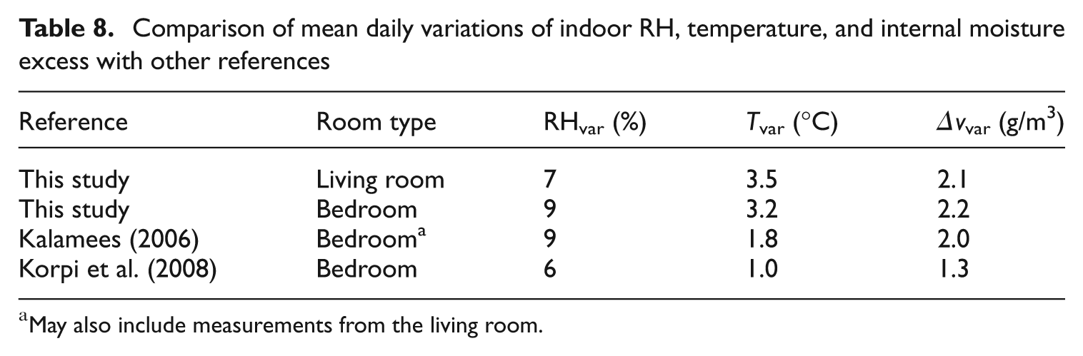
May also include measurements from the living room.
Measured weekly variations
As shown in Figures 10 and 11, the internal moisture excess is highly sensitive for changes in the outdoor air water vapour content (ve). This is due to the indoor air water vapour content (vi) not following these changes at the same rate. The hygroscopic inertia of interior surfaces and furniture dampens how quick vi can react on changes of ve. Since the internal moisture excess is the difference between vi and ve, this dampening can lead to variations of internal moisture excess from day to day even if the moisture production and the ventilation is the same. As shown in Figures 10 and 11, the hourly value of the internal moisture excess can even be negative.
Simulated diurnal variations
The simulations have several limitations. Among them, one of the most important being that it is chosen to be a one-zone model, assuming living room conditions in the whole house. Another important limitation is the definition of the moisture production profiles during the day. These profiles are, of course, only a few possible profiles for a living room; in reality, the profiles will be different for every single house and varying inhabitant behaviour. It should also be mentioned that furniture, bookshelves, and so on are not included in the simulations, thereby underestimating the real moisture buffer effect.
Even when considering these limitations, we can make some interesting observations. We see that only when the surfaces are of untreated spruce, we achieve a diurnal RH variation with daily variations similar to the field measurements. If the spruce is painted with alkyd paint, the moisture buffer effect is, on the other hand, almost completely lost. We also note that gypsum board has a much smaller moisture buffer effect than spruce, even when a rather vapour open paint is used. The case with gypsum board has almost doubled the daily variation of RH compared with the measurements.
It should however be mentioned that the difference in daily variation of internal moisture excess (Δvvar) between the case with gypsum board (Δvvar = 2.6 g/m3) and the measurements (Δvvar = 2.1 g/m3) is not so high. In addition, the difference in daily variation of internal moisture excess between the case with untreated spruce (Δvvar = 1.2 g/m3) and the measurements (Δvvar =2.1 g/m3) is however quite high, indicating that the untreated spruce, in fact, is overestimating the moisture buffer effect. One explanation to this different observation in regard to variation of RH and internal moisture excess could be that the indoor temperatures are not representing the real occurring indoor temperatures. There are some diurnal variations of the calculated indoor temperatures caused by, for instance, solar radiation through windows. The fact that the heating may be set on a lower level during night and work hours when the inhabitants are not present (in the living room) and thereby lower the temperatures when the moisture production is low are however not taken into account. This effect may give lower daily variation of RH.
About 20–30 years ago, it was rather common in single-family houses to have almost all internal surfaces of untreated wooden panel. Nowadays, this is not popular; most wooden panels are therefore painted with some type of paint with varying vapour resistance. Gypsum boards have, on the other hand, become more popular. This means that when simulating an ‘average’ Norwegian house with respect to daily variation of indoor air humidity, we would probably need a total moisture buffer capacity somewhere in between untreated spruce and painted gypsum board on all surfaces, which is also indicated by this parametric study. Preferably, the effect of furniture should be included by some manner. The findings also indicate that the daily variations of indoor temperatures, typically influenced by varying heating levels during the day, should be taken into account. The simulations also show the importance of defining reasonable moisture production profiles during the day.
Conclusion
Indoor air humidity loads in various types of houses have been investigated on the basis of measurements of RH and temperature during a period of 1 week. The measurements were made in 117 houses in the living rooms, bedrooms, and bathrooms.
Mean values and design values (10% critical level) for internal moisture excess has been investigated. It was shown that the internal moisture excess is dependent of the outdoor temperature, being approximately constant at temperatures below +5°C and decreasing as the temperature increases above +5°C. The highest levels of internal moisture excess were found in the bathrooms. The internal moisture excess was significantly higher in living rooms compared with bedrooms. The level of occupancy (person per heated area) was found to have an effect for the living rooms, giving significantly higher internal moisture excess for high occupancy compared with low occupancy. Some effects were also found for the age of the house and type of basic ventilation system, giving higher internal moisture excess for old houses and houses with inefficient ventilation systems. However, these differences were not significant. Based on these results, design curves for internal moisture excess have been proposed.
Typical daily variations of indoor RH, temperature, and internal moisture excess have been surveyed. It was found that the variation of RH and internal moisture excess generally followed the expected daily variation of moisture production due to the use of the house and the rooms. RH in the living rooms did however not vary much during the day. The mean daily variations of RH, temperature, indoor water vapour content, and internal moisture excess were relatively similar for the living rooms and the bedrooms, while the variations were higher for the bathrooms. The daily variations found in this study comply well with other studies. The dependency of the ventilation system and the seasonal variation of outdoor temperatures on the variations was found to be low.
It was found that the internal moisture excess, when calculated on an hourly basis, is highly sensitive to changes in the outdoor air water vapour content during the day and week. A general conclusion is therefore that measurements of indoor air humidity should be made on a long-term basis, that is, minimum 1 week of measurements as in this study. This is a necessity if internal moisture excess is to be used as a main parameter.
In addition to the field measurements, computer simulations analysing some of the factors influencing the diurnal variations of indoor air humidity were performed. Omitting the moisture buffer effect of furniture, bookshelves, and so on, a total moisture buffer capacity somewhere in between untreated spruce and painted gypsum board on all surfaces seemed to give daily variations for RH and internal moisture excess in accordance with the measurements. The simulations also indicate that the daily variations of indoor temperatures, typically influenced by varying heating levels during the day, should be taken into account.
Footnotes
Acknowledgements
This study has been performed within the ongoing SINTEF strategic institute project ‘Climate Adapted Buildings’. The authors gratefully acknowledge the Research Council of Norway for funding of the project.