
Abstract
This work is devoted to proposing a hybrid numerical–analytical method to address the problem of heat and moisture transfer in porous soils. Several numerical and analytical models have been used to study heat and moisture transfer. The complexity of the coupled transfer in soils is such that analytical solutions exist only for limited problems, while numerical solutions can deal with more realistic ones but at a higher computational cost. Therefore, we propose to implement analytical solutions where variations of temperature and moisture content are known to be almost nonvarying, while the numerical solution is implemented in the remaining region, near the boundaries. The coupling between solutions is performed assuming the continuity of both fields and fluxes at each interface. This strategy allows assuring the physical phenomenon occurring at the interface. Numerical experiments are performed, showing the accuracy, the efficiency, and the great potential of the method regarding applications in nonlinear soil problems.
Introduction
The ground may play an important role in estimating the energy consumption of low-rise buildings. Significant heat losses, from inside through the ground floor slab into soil, may imply a rise in the energy consumption (Rees et al., 2000). The heat loss via the ground is mainly calculated with pure heat transfer, as presented by Cichota et al. (2004), Claesson and Hagentoft (1991), Dos Santos and Mendes (2004), Nowamooz et al. (2015), and Rees et al. (2000). Most of these researches are based on the major hypothesis of none coupling effects between soil heat and moisture transfer. In particular, some cases consider the properties of soil as constant.
Although the soil is a porous material, the moisture transfer and its accumulation have a direct impact on the heat transfer. Moisture migration keeps the ground slab moist through the year (Rantala and Leivo, 2009). Janssen et al. (2004) showed that to precisely determine the heat losses, it requires simultaneous calculations with moisture content as they are closely related.
Other works (Bouddour et al., 1998; Janssen et al., 2002; Mulay and Worek, 1990; Rees et al., 2001) also proved that moisture content is a relevant parameter to be considered due to its mechanism of transport: as liquid water evaporates or condensates, it can absorb or release latent heat of vaporization, according to the process.
The heat and moisture transfer problem can be solved by numerical or analytical approaches, depending on the specified problem (Qin et al., 2006). The most used solution method is the numerical one due to almost none restrictions of boundary conditions (BCs), geometry, material properties, among other considerations. Examples can be found in the literature such as the finite-volume method, the finite-element method, and the finite-difference method (Berger et al., 2014; Mendes et al., 2002; Mikhailov and Özisik, 1994; Thomas et al., 1980; Yamazawa, 2001).
Concerning problems of heat and moisture transfer in porous soils, Liu et al. (2005) presented a 1D mathematical model based on the volume-averaging method. The authors validated their numerical method with an experiment conducted under natural environmental conditions. Dos Santos and Mendes (2006) presented a complete analysis of soil simulation with building interactions. They applied a numerical method to compute the 3D heat and moisture transfer in soils, with the finite-volume method. Their work included the effects of rain on the heat losses from the ground to the building. Coelho et al. (2009) developed a succeeded approach based on neural network and clustering method to compute the temperature and moisture fields in unsaturated soils. Mendes et al. (2012) compared in situ soil measurements with two different numerical models, the coupled Philip and De Vries model prescribed in Domus (Mendes et al., 2008) and a decoupled one, in order to validate them. Both numerical models succeed in predicting the temperature and the moisture content profiles.
Analytical methods as the ones proposed in Abahri et al. (2011), Chang and Weng (2000), Qin et al. (2006), and Ribeiro et al. (1993) have some disadvantages such as simplifications of the real physical phenomenon and the fact that variable properties and transport coefficients have to be considered linear. Nevertheless, the analytical solution has important advantages (Cichota et al., 2004) such as the reduction of the computational cost, especially when the variations of temperature and moisture content profiles must be investigated over significantly long periods (Lee et al., 2010).
Even with the development of these methods, modeling the coupled phenomenon of heat and moisture transfer in soil faces important issues. Indeed, the computational cost rises importantly when computing the solution due to the following problems among others:
The definition of the BCs at the bottom surface of the soil domain is a difficult question. Most of the works (Coelho et al., 2009; Dos Santos and Mendes, 2006; Janssen et al., 2004; Thomas et al., 1980) consider an adiabatic condition, assuming that after a certain depth, there are no temperature and moisture content gradients. This hypothesis imposes the modeling of a large spatial domain (around 10/20 m), whereas the interesting dynamics region lies at the first decimeters (Rantala, 2005).
The consideration of moisture transfer imposes strong nonlinearities (Dos Santos and Mendes, 2006; Thomas et al., 1980). Contrarily to the analytical approach, numerical methods can consider the moisture dependency of physical properties. Depending on the type of numerical approach, one requires very short time steps to compute the solution with sufficient accuracy. Thus, for long-time simulation (for one or several years), considering large spatial domain, the computational cost increases.
Thus, to deal with all these issues, traditional numerical methods have to be improved or even replaced by other models (Pallin and Kehrer, 2013). The objective of this work is to propose an innovative mathematical method to solve nonlinear heat and moisture transfer in soils, with a special focus on the application to large domains. A hybrid method is proposed based on the combination of analytical and numerical approaches. This type of approach was already applied by Godinho et al. (2011) for solving the problem of underwater sound scattering by an elastic shell. Lee et al. (2010) proposed a similar approach, dealing only with analytical solutions, for solving heat and moisture transfer through a two-layered wall.
As a matter of fact, it can be noted that temperature and moisture content gradients are greater near the surface, and deep into the ground, temperature and moisture distributions are almost uniform (Coelho et al., 2009). This behavior provides a good opportunity for the hybrid method. The strength of the numerical models can be used near the surface, to perform accurate computations where the effects of the nonlinearities are more intense. However, the analytical solution can be used for the deeper layers where the diffusion process is relatively smooth.
In this work, section “Coupled heat and moisture transfer in soils” details the mathematical model of heat and moisture transfer in unsaturated porous soils. Fundamentals of the hybrid method are presented in section “Hybrid analytical–numerical method.” Numerical results are performed and discussed in section “Computational simulation.” Then, in section “Final remarks,” conclusions are addressed and future perspectives are provided.
Coupled heat and moisture transfer in soils
Mathematical formulation
Dos Santos and Mendes (2006) adopted the Philip and De Vries equations for the heat and moisture transfer in soils, with

and the mass conservation as

where
The BCs at the surface are considered to be in contact with the internal air of the building and can be mathematically described by the following equations (Dos Santos and Mendes, 2006; Mendes et al., 2012)
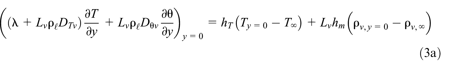

with

where


with


In these equations, the subscript
On the other side, an adiabatic condition is assumed


At the initial condition, the temperature and the moisture content values are


These values are chosen according to the problem. They can be constant values or functions of y. Other conditions will be necessary to the use of the hybrid method and need to be presented. The Neumann condition gives


with


The dimensionless representation
This subsection presents the dimensionless form of the linear mathematical model. To adimensionalize the problem, the following dimensionless quantities are defined:
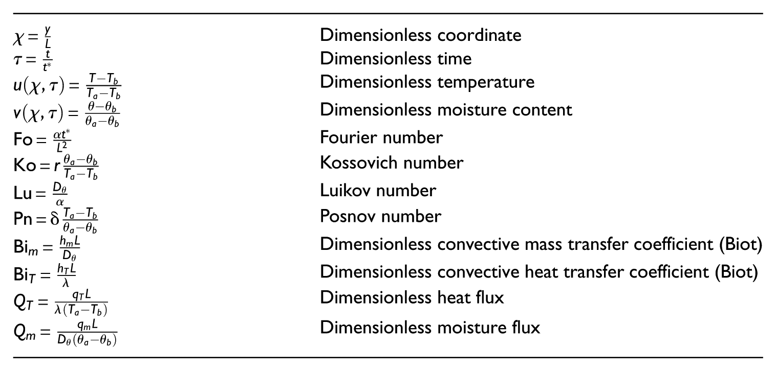
where
The dimensionless problem of equations (1) and (2) is written as (Mikhailov and Özisik, 1994)


Considering the subsequent BCs at the surface


where


At the bottom, the dimensionless forms are


Initial conditions, represented by equations (8a) and (8b), are now written as follows


The other BCs in the nondimensional form are


Hybrid analytical–numerical method
The hybrid method proposed here consists in decomposing the domain of the differential governing equations in two subdomains, separated by an interface. The location of this interface is not randomly chosen, and its location is determined by a pre-simulation of the problem, with the numerical method. After this, each one of the subdomains is solved analytically or numerically, developing their solution procedures alternately. Thus, through an iterative process, the approximation of the original problem is achieved by a composition of both subdomain solutions (Quarteroni and Valli, 1999; Shanthikumar and Sargent, 1983).
Analytical method
There are several methods of analytical solutions that have been applied to solve the heat and mass transfer problem (Abahri et al., 2011; Chang and Weng, 2000; Lee et al., 2010), as the separation of variables, the integral transforms, the Laplace transform, and others techniques. The one applied in this work is the separation of variables (Özisik, 1993), which can be found in Appendix 2. This approach is used due to the use of the hybrid method, which requires the update of the initial condition of the solution at each increment of time. The analytical method is particularly interesting for its robustness, which allows reducing the number of spatial and temporal nodes without losing accuracy. There is almost no restriction of stability.
Numerical method
The numerical method applied in this study is based on the finite-difference approach, with an implicit second-order scheme, of the Crank–Nicolson type (Crank and Nicolson, 1947). It is used as part of the hybrid method and as a reference solution to validate the features of the hybrid approach.
Illustration
To clarify the hybrid method, consider the domain
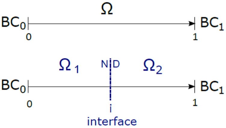
Schematic diagram of the domain decomposition in two parts, where N corresponds to the Neumann condition and D to the Dirichlet condition at the interface (i). Besides, the BC corresponds to the boundary condition at outer surfaces with 0 and 1 corresponding to each side.
It is important to mention that material properties are considered constant in subdomain 2 due to the analytical solution but nonlinear in subdomain 1 due to the numerical solution. This separation will be defined according to the variation of the material properties of the soil (see “Introduction”).
When the domain is decomposed, an interface between subdomains is created (called hybrid interface henceforth), and (i) the continuity of the field and (ii) the conservation of the flux must be ensured (Özisik, 1993). The mathematical formulation of these assumptions for the temperature is given by (De Freitas et al., 1996)

Superscripts − and + represent the left and the right sides of the interface, respectively. The continuity of the field and the conservation of the flux are also assumed for the moisture content.
To satisfy equation (17), at one side of the interface, a Neumann BC is assumed. Then, on the other side, a Dirichlet BC is considered. It would be more common to assume a Robin condition at the interfaces. Although, it is not employed here because of the eigenvalue problem originated from the analytical solution. It yields a transcendental equation whose resolution cannot be systematically computed for any particular value of the BC without degrading seriously the computational advantage of using an analytical solution.
Thus, taking into account the hybrid interface, the boundaries of the


where


And the boundaries of


Subscripts 1 and 2 represent subdomains
Since


where
For the first time step, the algorithm runs the numerical solution considering the first guess of the flux at the hybrid interface (equation (21c)). Once the temperature and moisture content profiles are computed for

where
The hybrid method algorithm can be synthesized in Algorithm 1.
Algorithm 1
Solution of the hybrid method for the two subdomains.
Initializing of
Returns
Returns
Time increment:
Fields update:
Computational simulation
Case study
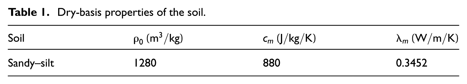
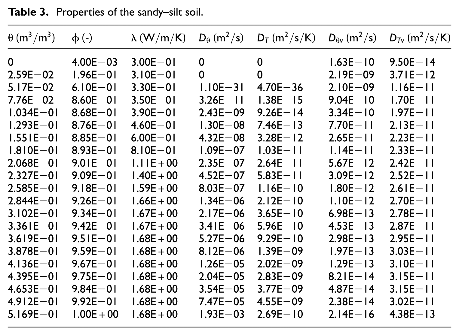
To study the features of the hybrid method for heat and moisture transfer in soils, a unidimensional case study of 20 m length is considered. Figure 2 presents the geometric configuration of the problem to be simulated. The dry-basis properties of the sandy–silt soil are presented in Table 1, from Oliveira et al. (1993). The nonlinear properties can be found in Table 3.
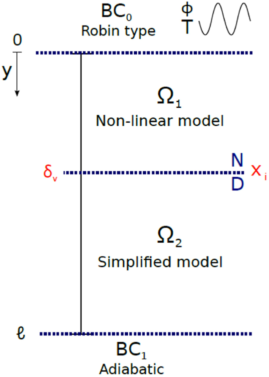
Schematic representation of the ground problem.
Dry-basis properties of the soil.
The surface, at y = 0, is subjected to Robin BCs, mathematically represented by equation (3). For the surface conditions, it was considered a yearly average temperature of 288.15 K with a daily and a yearly variation of 5K. For the relative humidity, it was considered a daily variation between 60% and 80% (Dos Santos and Mendes, 2006; Mendes et al., 2012). Summarizing it


The soil is initially at a constant temperature of
Adimensionalization
To write the problem in the nondimensional form, some characteristic values must be adopted. The characteristic time is


Simulation procedure
The simulation procedure performed by the hybrid method is divided into two steps: (i) perform the pre-simulation to chose the hybrid interface and (ii) simulate the hybrid analytical–numerical method to compute the fields.
In the framework of the hybrid method, the whole domain is divided into two parts, subdomains
The linear pre-simulation is performed with the numerical method presented in section “Numerical method.” The dimensionless numbers are Ko = 2.3, Lu = 0.01, Fo = 1, and Pn = 13. These values are obtained from the maximum property values (Table 3) referent to the range of the relative humidity. Biot numbers are assumed to be
Some additional simulations are executed, considering the linear case and the nonlinear, just to the necessity of considering the nonlinearities. With these, it is possible to understand how well the hybrid method is suitable in this case. The difference between the linear and the nonlinear pre-simulation is that the dimensional numbers Ko, Lu, Pn, and Fo are varying at each time step according to the moisture content.
Numerical results and discussion
The importance of considering nonlinear properties
In Figure 3, the differences for the case study between a pre-simulation with constant properties and nonlinear ones are highlighted. It displays the evolution of moisture content over the time, presented on the soil surface (
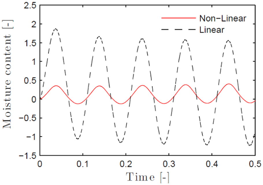
Evolution of the moisture content at the soil surface.
In addition, Figure 4 compares the linear with the nonlinear case but presenting the dimensionless moisture as a function of the space. The nonlinearities are stronger at the surface in contact with air, that is,
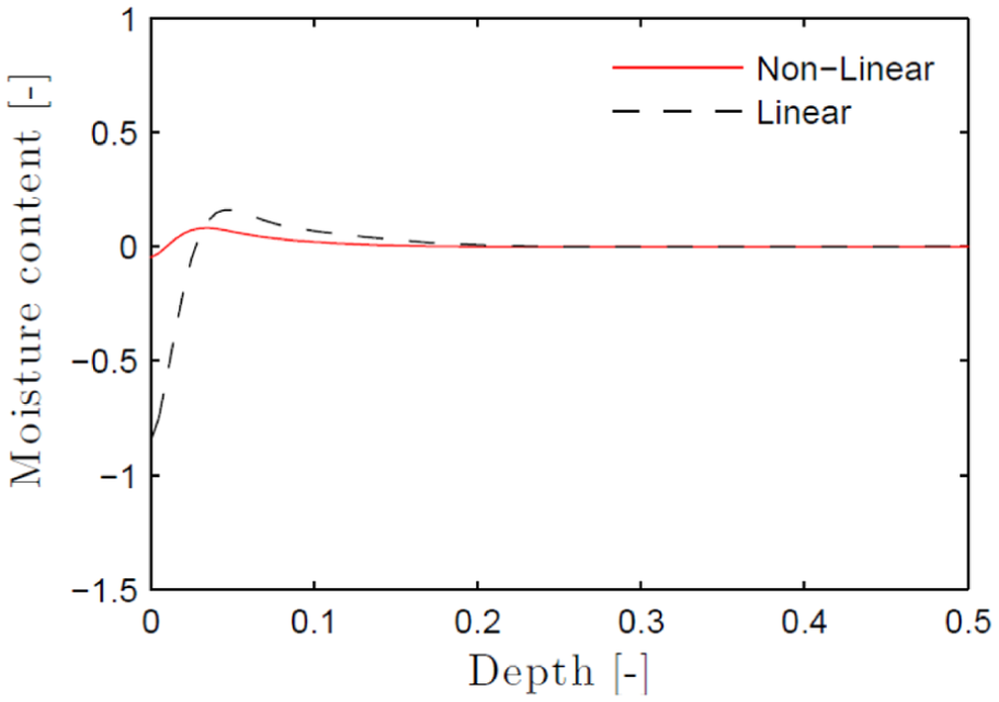
Moisture content profile for
Pre-simulation: definition of the hybrid interface
This type of behavior is particularly suitable for the hybrid method. The numerical part will be implemented in the part where the nonlinearities are stronger. As noted in Figure 4, the nonlinearities are stronger near the surface. The problem is the location of the interface that will separate both subdomains. For this, a pre-simulation is performed with the numerical method, for a dimensionless time
Given the results of the pre-simulation, the mass and temperature fields and the fluxes are analyzed. First, it seeks where the fluxes are near to zero (with a given tolerance) and then where the second derivatives of the fields are close to zero

If equation (25) is satisfied, then the location
Figure 5 presents the location where the condition given by equation (25) is satisfied as a function of time. There are two logical values to be selected, the highest value
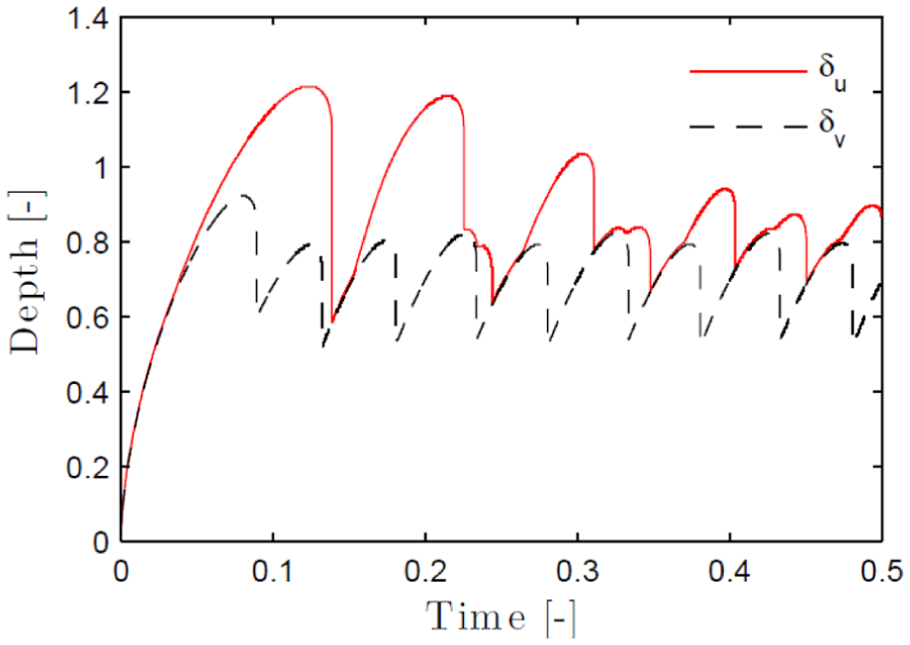
Penetration depth of temperature and moisture content gradients.
Comparison of hybrid and numerical methods
Using previous results, the interface location is first set as
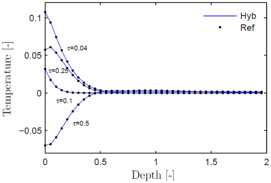
Temperature profiles for different time instants.
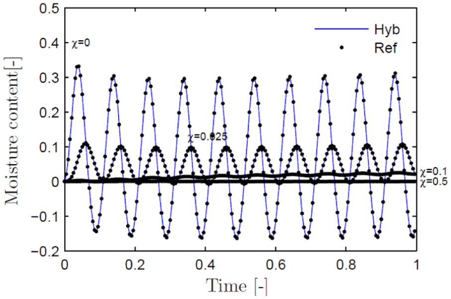
Moisture content evolution at different depths,
If the pre-simulation is considered on the computational cost of the hybrid method then, in this case, 20s must be added to the final simulation time. More details of the computational cost are provided in section “Computational cost.”
Figure 8 presents the root mean squared error (RMSE), calculated among the time for each node of the grid. This error is given by the following formulation (Cichota et al., 2004)
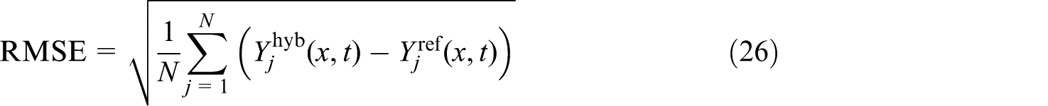
where
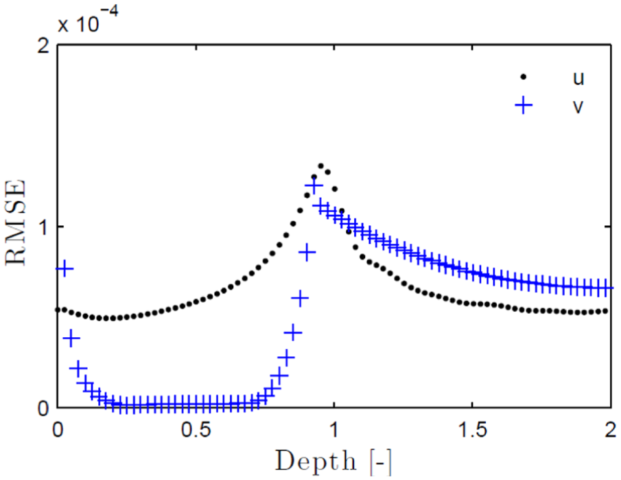
Error computed for temperature (u) and moisture content (v), considering
For the hybrid simulation with the interface located at
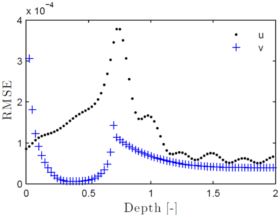
Error computed for temperature (u) and moisture content (v), considering
In Figure 10, the error is presented as a function of time for the case where the interface is located at
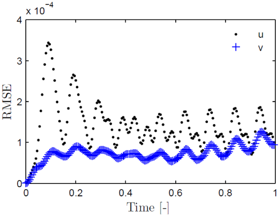
Error in function of time computed for temperature (u) and moisture content (v), considering
A numerical model using adaptive mesh has a similar approach. The mesh discretization is more refined where the nonlinearities are higher at the surface, whereas the mesh size increases deep in the ground. Nevertheless, the analytical solution may not have restrictions regarding stability or accuracy.
Computational cost
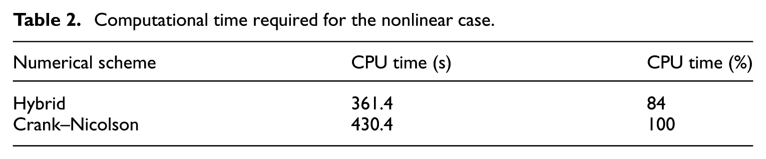
As previously mentioned, the hybrid method is faster than the traditional Crank–Nicolson scheme, when they are directly compared as shown in Table 2 for the CPU time. Simulations were performed in a computer with a processor Intel® Core™ i5-4460, with 8 GB of RAM memory, and coded in MATLAB (2013). If we add the computational time of the pre-simulation, the total gain with the hybrid method drops from 16% to 12%.
Computational time required for the nonlinear case.
Properties of the sandy–silt soil.
In the aftermath, the number of operations will be analyzed, since it presents another way to compare the computational cost. Considering the hybrid method, the domain over equations (11a) and (11b) is separated into two parts. The part calculated with the analytical solution has some simplifications, which leads to the following governing equations for this subdomain


Thus, this representation substitutes the original problem, given by equations (11a) and (11b), by two new differential linear equations. With these assumptions, there are no more updates of properties for this part in which the coupling effects of moisture over the temperature are neglected. It is important to note that these differential linear equations can be solved using analytic solution, as presented in the hybrid method. As a consequence, solving the two linear differential equations implies a lower computational cost than solving the original ones. At the same time, this is not the only part concerning to the hybrid method, and a deeper analysis must be carried out.
Notations
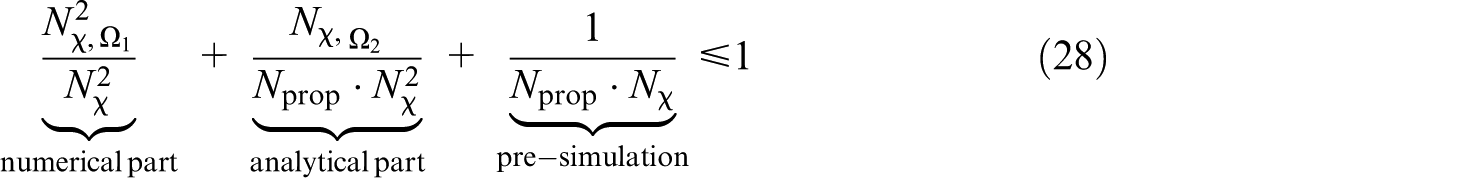
The first term corresponds to the numerical part of the hybrid method. Thus, to make the sentence truthful, it is necessary that
The analytical part corresponds to the second term of equation (28). The higher the number of properties to update, the lower this term. In addition, as this part is simulated analytically, the number of nodes does not influence the accuracy of the solution, so that they can be decreased as much as necessary. However, as the analytical solution is running with the numerical part, its advantage is lost due to the way it is implemented, with time steps.
Furthermore, the third term of equation (28) concerns to the pre-simulation cost. Similar to the second term, the higher the number of properties to update, the lower this term. In addition, if the properties vary also with the temperature, the computational cost of the hybrid method will be even lower. In summary, the hybrid method offers an interesting approach when the diffusion process is very slow, and a great number of properties must be updated at each iteration.
Final remarks
Conclusion
This work proposed a hybrid method to compute the heat and moisture transfers in porous soils. It consists of finding an area where the second derivative of the moisture content is approximately null. In this area, a simplification of the problem is considered and calculated with an analytical solution, leading to a reduction of the computational cost.
The method has been illustrated in a 1D nonlinear case of heat and moisture transfer in unsaturated soils. A 20-m domain was considered with a 10-year time simulation length. The analytical solution is implemented deep into the ground, where variations of properties can be neglected. The numerical solution is implemented where the effect of the nonlinearities is more intense. Both solutions are connected through an iterative process which is performed until reaching the convergence.
Since no analytical solution exists for the complete problem, its verification was performed against a numerical model. It has shown an excellent agreement.
Furthermore, the domain separation may reduce calculations, considering the properties to be constant 5 m below the surface and thus ignoring the second derivative of moisture content in this part. The hybrid method offers an interesting reduction of the computational cost when the diffusion process is very slow, and a great number of properties varies with the field. These conditions are reached in most problems of soil heat and moisture transfer and, therefore, suit well to the hybrid method.
Further investigation is needed to improve the hybrid method. Particularly, the determination of the hybrid interface location can be enhanced with a process calculating alongside the hybrid method, updating the position of the interface among the time iterations. Another point is the way both domains are coupled; perhaps, if the domains are overlapped, the model can become more robust. In addition, modeling the problem in two or three dimensions with the hybrid method, the computational cost can be significantly reduced.
Outlooks
The methodology presented in this manuscript considered only unidimensional problems. Given the promising results, it can be applied in the context of whole-building energy simulation, aiming at estimating the building energy consumption, where the diffusion transfer in the spatial domains (wall and soils) is assumed as unidimensional. However, in some practical cases, 2D (or even 3D) transfer might be considered for a more accurate assessment of diffusive transfer phenomena in building foundations.
The hybrid approach can be used in such cases. The two subdomains are set as illustrated in Figure 11. The first domain is defined where the field has high magnitudes of variations. In this domain, a numerical model considering 2D transfer and nonlinear material properties can be used. In the second domain, the variations of the dependent variable are assumed to be negligible. The analytical solution as the ones proposed by Comini and Lewis (1976) and Guimarães et al. (2010) can be used in this second domain.
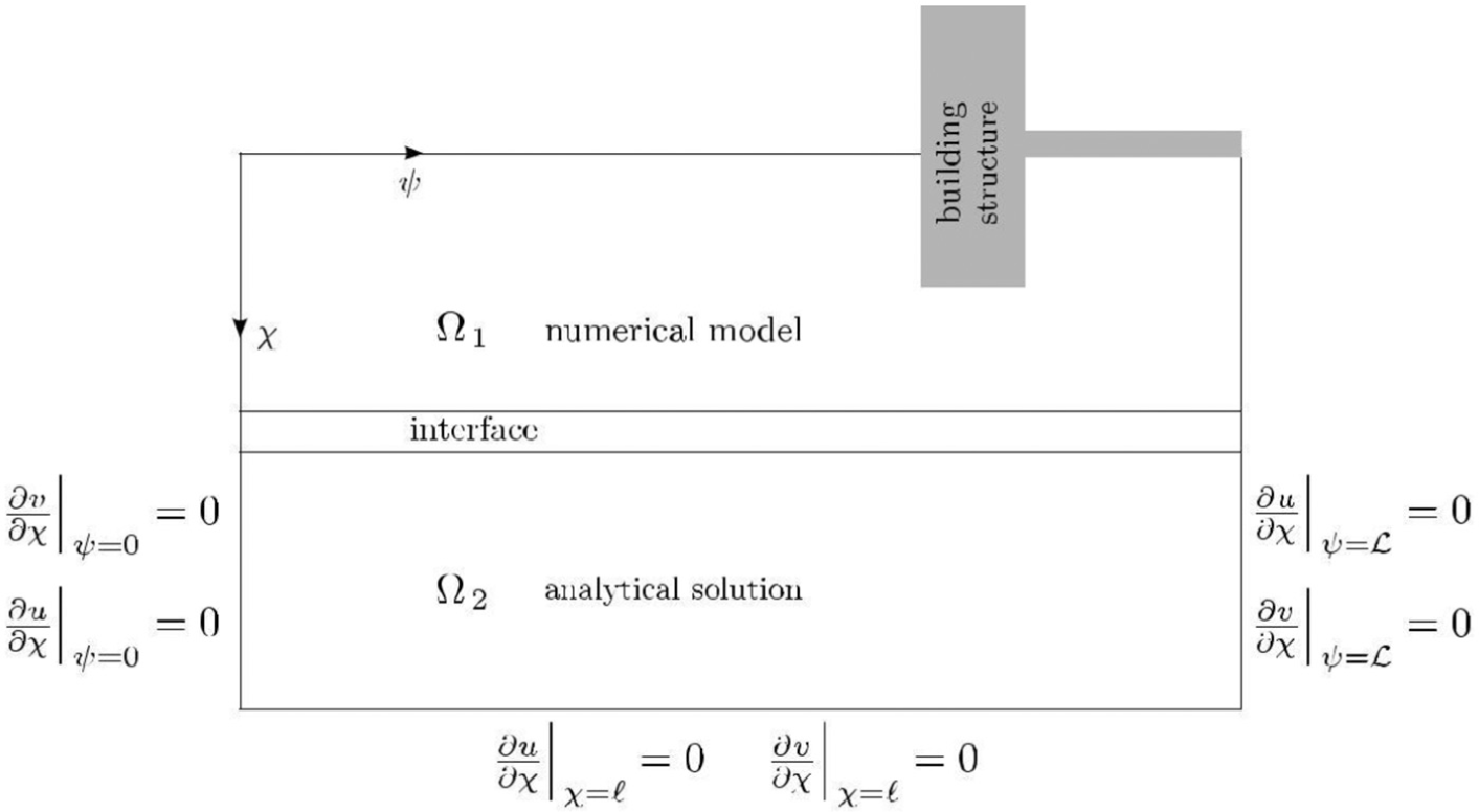
Schematic representation of the ground problem considering 2D transfer.
Another possibility that deserves investigation is to consider an analytical solution for unidimensional diffusive transfer for the simplified model. Indeed, the magnitudes of the variations of the field have to be assumed small compared to the ones within the first domain. Moreover, due to adiabatic BCs, the fluxes are unidimensionally directed (over ψ).
An important issue when considering 2D transfer is the interface of the hybrid model. As for the unidimensional approach, the continuity of the fluxes and of the dependent variables fields is ensured at the interface by equation (17). It may be advantageous to have overlapped domains to guarantee this condition. The location of the interface can be determined with a pre-simulation, similar to what has been done for the unidimensional case presented here, or, for practical reasons, it could be determined by other means. The option is implementing the hybrid algorithm in a such way the interface moves along the simulation, supported by the computations of the fluxes to determine its location. As we believe that the results are promising, research for 2D transfer will be conducted in the near future.
Footnotes
Appendix 1
Appendix 2
Declaration of conflicting interests
The author(s) declared no potential conflicts of interest with respect to the research, authorship, and/or publication of this article.
Funding
The author(s) disclosed receipt of the following financial support for the research, authorship, and/or publication of this article: This work was supported by the Brazilian Agencies CAPES of the Ministry of Education and CNPQ of the Ministry of Science, Technology and Innovation.