






Abstract
In Europe, a large share of the building stock is old, with approximately 85% of buildings constructed before the 1970s and 64% exhibiting poor energy performance. Achieving the decarbonization of the building sector by 2050 requires comprehensive and socially inclusive energy efficiency strategies. The revised Energy Performance of Buildings Directive strengthens energy efficiency requirements while explicitly addressing energy poverty, particularly by protecting vulnerable households from excessive rent increases following renovations. This study proposes a multidimensional framework that integrates Urban Building Energy Modeling with socio-economic analysis to evaluate energy retrofit scenarios and their impacts on energy poverty in the city of Turin, Italy. A physics-based UBEM was calibrated using hourly heating consumption data from 125 residential buildings and further enhanced through Machine Learning to extend predictions across multiple retrofit configurations. To improve the representation of boundary conditions in physics-based models, a simplified QGIS-based solar gains simulator was developed to estimate solar irradiation on roofs and façades using 2.5D building footprints enriched with height, orientation, and shading information. Solar gains are calculated separately for horizontal and vertical building components, explicitly accounting for urban shading effects and sky view factors. The solar model validation demonstrated a good agreement with measured solar radiation data on horizontal surfaces and CitySim Pro simulation on vertical envelopes with MAPE of 2%–3% and 6%–23%, respectively. Energy poverty was assessed using two widely adopted indicators: the 10% income threshold and the Low Income High Cost indicator. Results indicate that wall insulation is the most effective single retrofit measure, reducing energy poverty levels from a baseline of 14.4%–17.6% to approximately 6.3%. On the other hand, a fully incentivized global retrofit can reduce the energy poverty index to as low as 2.2%. However, the current annual renovation rate of around 2% significantly constrains the large-scale impact of these interventions.
Keywords
Introduction
After being overlooked and marginalized for many years, energy poverty has increasingly gained recognition as a key policy concern within the European Union (EU; Bouzarovski et al., 2021). The commitment to reducing energy poverty was established by the United Nations (UN) as Sustainable Development Goal 7 (SDG 7), which seeks to ensure universal access to affordable, reliable, sustainable, and modern energy by 2030. In Europe, the EU Energy Poverty Advisory Hub (EPAH) supports member states in addressing this issue, with a particular emphasis on providing additional support to vulnerable populations (Che et al., 2021).
Until now, energy poverty has been defined in various ways. Historically, to measure energy poverty, the work of Boardman in 1991 was a reference (Boardman, 1991), introducing the “10% threshold.” According to her, households spending over 10% of their income on energy are considered energy-poor. A more nuanced measure is the Low Income High Cost (LIHC) indicator, identifying households as energy-poor if they are both income-poor and face above-median energy costs (Al Kez et al., 2024; Hills, 2012). This approach distinguishes energy poverty from general poverty by highlighting the energy-specific burden. On the other hand, to quantify energy poverty, the EU Commission grouped indicators into two categories: affordability indicators (e.g. inability to heat homes, bill arrears) and structural indicators (e.g. housing conditions, income levels; European Commission, 2020).
Poorly insulated buildings often require higher energy needs to ensure indoor comfort, placing a disproportionate burden on low-income households. This has led to increased focus on building retrofits as a means of lowering energy consumption and improving living standards (Fabbri et al., 2023). The Energy Performance of Buildings Directive IV (EPBD IV; European Commission, 2024) also stresses that inefficient buildings correlate strongly with energy poverty and that renovation must be inclusive, preventing post-renovation displacement or unaffordable rent increases. However, the relationship between building characteristics and energy poverty is still an emerging area of research.
To evaluate retrofit strategies effectively, dynamic energy modeling is essential. These models simulate buildings’ energy performance using different methodologies: physics-based approaches (white-box models), data-driven techniques (black-box models), or a combination of the two (grey-box models; Li and Wen, 2014a, 2014b). In situations where empirical data are limited, particularly at the urban scale, white-box models are useful. Physics-based Urban Building Energy Modeling (UBEM) adapts traditional simulation techniques to the city scale by incorporating GIS-based data on building geometry and energy use. Although such models require assumptions regarding parameters like occupancy behavior and the types of technological systems in place, which may influence their accuracy, they still offer valuable insights when applied in an aggregated, large-scale use. These tools are instrumental in assessing the impact of renovation scenarios on energy consumption and, consequently, the potential to reduce energy poverty.
A distinctive aspect of this study is its integration of bottom-up UBEM with socio-economic analysis. This dual approach allows for a comprehensive understanding of how building features affect energy use and contribute to energy poverty. The research assesses different retrofit scenarios through a cost-optimal analysis, considering not only energy savings but also financial viability and social equity.
Several previous studies have investigated the integration of UBEM with socio-economic and energy vulnerability assessments. For instance, Kelly et al. (2020) developed a composite indicator to evaluate heating energy poverty risks under different environmental policy scenarios, while Fabbri et al. (2023) explored the role of building envelope retrofits in reducing energy poverty in Italian social housing. Sherif and Rakha (2023) proposed the integration of socio-economic vulnerability indicators into UBEM workflows to support intervention strategies for underrepresented communities. However, existing studies generally rely on simplified assumptions about urban morphology and boundary conditions within the UBEM framework. In addition, recent review studies highlighted that socio-economic integration in UBEM applications remains limited and insufficiently explored. In this context, the present study contributes to the literature by integrating a detailed physics-based UBEM and socio-economic energy poverty indicators within an urban-scale framework.
The performance of UBEMs strongly depends on the accuracy of their input data, as providing concrete boundary conditions is highly important. One of the most important boundary conditions in buildings’ energy consumption is the solar gain of their envelopes. In this study, one of the crucial aims was to develop a methodology to analyze solar gains on vertical and horizontal components of the buildings. To address this, a simplified GIS-based solar irradiance simulator is designed to compute solar gains in 2.5D space on building facades and roofs, accounting for urban shading and view factors.
The focus on solar gains is particularly important because they can directly influence heating demand. In dense urban areas, solar exposure varies significantly depending on building orientation, height, and surrounding obstructions, which can substantially modify façade-level heat gains. Simplified assumptions or uniform radiation inputs may therefore lead to biased estimations of energy demand at the building scale. Since the objective of this study is to evaluate retrofit strategies and their impact on energy poverty, it is essential to accurately estimate solar gains to avoid overestimating heating needs and misrepresenting potential energy savings. By improving the representation of solar radiation at the envelope level, the reliability of the UBEM results is strengthened, leading to more robust economic and social assessments of retrofit interventions.
In this light, the core novelty of the current research lies in the development of the simplified GIS-based solar gain simulation in 2.5D space to estimate façade and roof solar gains. This is crucial for physics-based UBEMs because solar gains significantly affect heating consumption. This improvement helps to improve boundary condition estimation for physics-based UBEM and, at the same time, reduce uncertainty in heating consumption estimation. Also, the novelty of this research extended to the development of an integrated urban-scale framework that couples bottom-up UBEM with socio-economic vulnerability analysis to evaluate retrofit strategies not only in terms of energy performance and cost optimality, but also their effectiveness in alleviating energy poverty.
This study focused on the city of Turin in Italy, where the relationship between the energy performance of buildings and the socio-economic vulnerability of families is examined. The actual energy consumption is analyzed through process- and data-driven models, and the retrofit scenarios are evaluated in terms of investment costs, savings, affordability, and overall impact on energy poverty alleviation. Focusing on the urban context of Turin, this study provides local insights into how energy performance upgrades can alleviate energy poverty, offering a model for targeted, equitable, and effective retrofit policies in similar urban settings.
Case study
This work investigated the residential building sector in the city of Turin, analyzing its energy consumption, the expenditure on energy services, and the energy poverty of families. The actual and future scenarios with retrofit interventions are explored in this context.
Turin is one of the major Italian urban centers located in the northwestern part of Italy and is characterized by a temperate climate. Its climate is classified within climatic zone E, with 2617 Heating Degree Days (HDD with base temperature of 20°C) and 84 Cooling Degree Days (CDD with base temperature of 26°C). The urban fabric comprises approximately 44,289 building units, of which residential structures constitute around 82% of the total stock. Notably, approximately 29% of these buildings exhibit mixed-use functionality, typically incorporating commercial or office spaces on the ground or first floor.
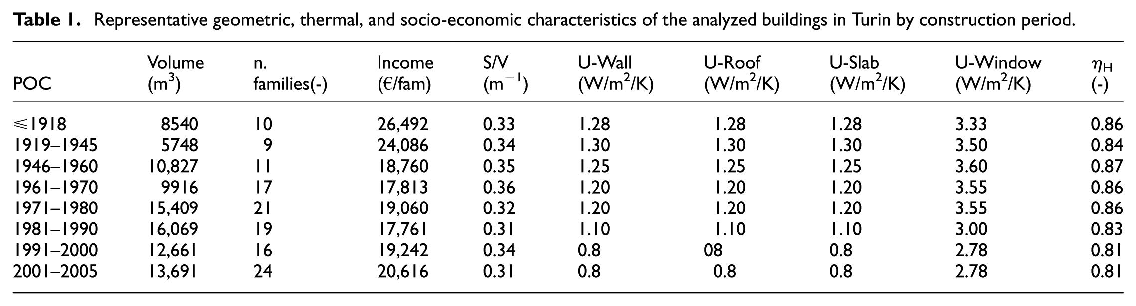
For the energy consumption of space heating (H), monthly and hourly data were available for 4870 and 170 buildings, respectively, from 2019 to 2024. In this study, a target investigation period consisting of a continuous 12-month timeframe (May 2022–April 2023) was selected. These data were utilized for the development, calibration, and validation of process- and data-driven UBEMs. For the geometrical and typological characteristics of the buildings, technical maps of Turin were used (Geoportal of the Municipality of Turin, 2025). Table 1 describes the main characteristics of the residential buildings analyzed, grouped by the periods of construction up to the year 2005 (after 2005, the number of buildings with measured energy consumption data was inadequate to conduct any analysis). The consumption data mainly refer to large-compact buildings of six floors and 8400 m3 with 22 apartments connected to the District Heating Network (DHN) and equipped with a temperature regulation system for each zone or room. The apartments have a surface of 88 m2, are occupied by 2.1 people with an income of 28,000 €. The U-values were evaluated considering the Italian energy savings laws and the EPCs’ database for the city of Turin (Mutani and Todeschi, 2021).
Representative geometric, thermal, and socio-economic characteristics of the analyzed buildings in Turin by construction period.
For Domestic Hot Water (DHW) consumption, the Italian standard UNI/TS 11300-2 (UNI Ente Italiano di Normazione, 2019) was used to evaluate the volume of water at 48°C required as a function of the net area of the dwellings. For the hourly profile, the ASHRAE 90.2 (1994) Standard was used.
Regarding electricity consumption (E), the monthly profile for the province of Turin was utilized, which shows an average consumption of residential users in the last 3 years of approximately 2700 kWh/year (ARERA, 2024). It is necessary to add that in Turin, cooling energy is not supplied through the district network. Cooling demand in residential buildings is generally limited. When it is present in a residential building, typically powered by individual electric systems. Consequently, cooling energy consumption is indirectly reflected in overall electricity consumption.
For the analysis on energy poverty, the main reference is the Directive (EU) 2023/1791 (European Union, 2023; at Article 8, paragraph 3), promoting the reduction of consumption for families in energy poverty status, vulnerable customers, and people living in low-income households or social housing. In the Piedmont Region, the “Statistics on Income and Living Conditions” (Eu-Silc) have been monitored for the year 2022 (ISTAT, 2023):
- the inability to keep the home adequately warm: 13%
- the arrears on utility bills: 5.1%
- the total population living in a dwelling with a leaking roof, damp walls, floors, or foundation, or rot in window frames or floor: 13.3%
- at-risk-of-poverty rate (cutoff point: 60% of median equivalized income after social transfers, 18,472 € (Eurostat, 2022)): 15.4%.
In 2024, the Ministry of Economy and Finance published the number of taxpayers, the total declared income, the average income per taxpayer, and the distribution of income in the municipality by different income classes. The average income in Italy is 24,829 €, with 28,889 € for Turin. These data are distinguished by the postal code zones of every city, including Turin.
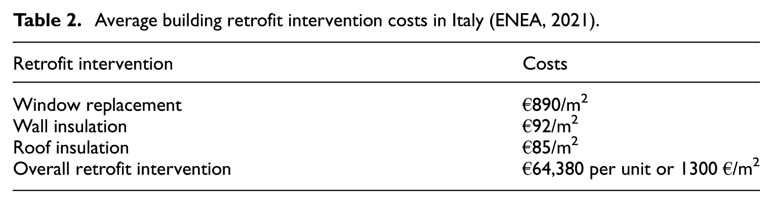
Finally, to examine actual and future retrofit scenarios, the energy prices and the costs of retrofit interventions were analyzed. About energy prices, average values have been considered: 0.23 €/kWh for electricity, 0.133 €/kWh for natural gas, and 0.117 €/kWh for district heating (DH; The Consumer Protection Center, 2025). Table 2 synthesizes the average costs in Italy for the different interventions of building retrofit.
Average building retrofit intervention costs in Italy (ENEA, 2021).
For advanced retrofit interventions, the analysis follows the provisions outlined in the Super Bonus legislation (Agenzia delle Entrate, 2022). Under this framework, the maximum eligible expenses for single-family homes are set at 50,000 € for building envelope upgrades. As specified by the regulation, for interventions carried out in 2025, 65% of the total investment costs are recoverable through tax deductions.
Methodology
The study follows a three-phase methodology (see Figure 1) designed to examine the relationship between building energy use, retrofit strategies, and energy poverty reduction. Central to this approach is the integration of spatial and place-based factors, including building typologies, climatic conditions, and socio-economic characteristics, which ensures that the analysis is sensitive to local variations across different areas. Geospatial data processing and mapping were conducted using QGIS, enabling a detailed spatial representation of energy dynamics. By analyzing the site-specific approach, the research offers a detailed understanding of how renovation measures can effectively address energy poverty at the local scale. In the following, an in-depth description of each analysis phase is provided.
1. Pre-modeling: This step comprises three sub-phases. Open-source, site-specific data were gathered for urban-scale energy modeling. This includes the collection and calculation of building features (e.g. volume, heat-loss surface, surface-to-volume ratio, thermal transmittances, exposed walls and their azimuth angle, roof segments and their slope and azimuth angle), socio-economic data (e.g. population, households, income, energy price; ISTAT, 2021; Ministero dell’Economia e delle Finanze, 2024), climatic variables (e.g. air temperature, solar radiation; Living Lab Politecnico di Torino, 2023), and measured energy consumption. The hourly energy consumption of 125 buildings helped calibrate and optimize the simulation models, ensuring that the outputs accurately reflected real-world buildings’ energy behavior at the urban scale. Also, the use of mainly open-source data ensures the replicability of the methodology.
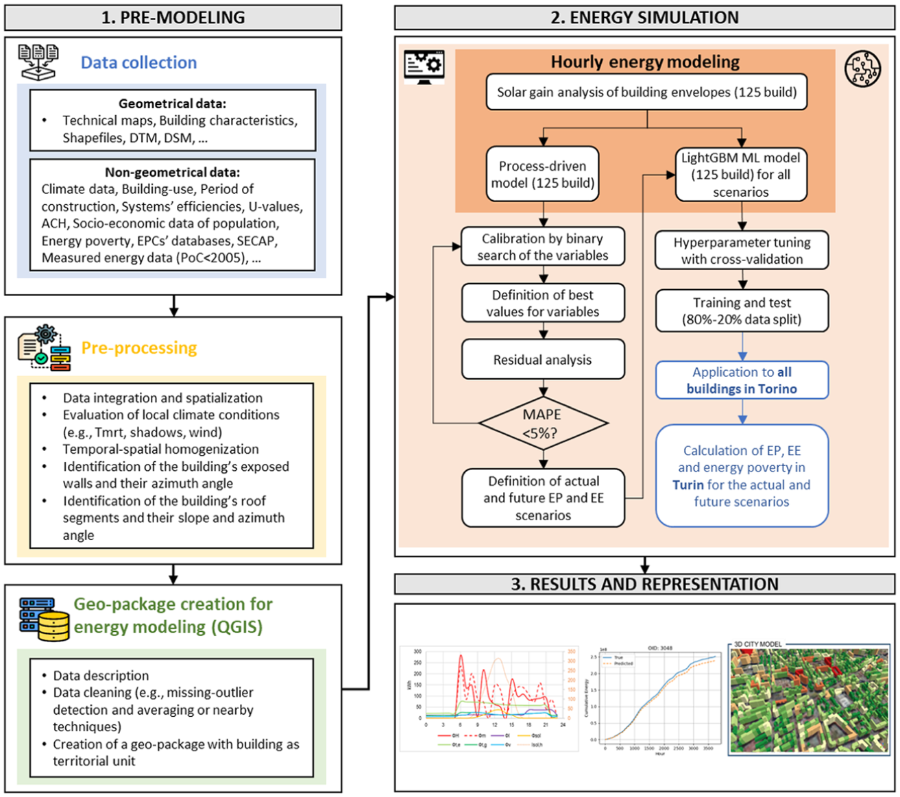
The flowchart of the applied methodology.
Then, the building data was corrected, removing anomalies and organizing the cleaned data into a geo-package to support GIS-based energy modeling.
2. Energy simulation: Like the previous stage, this phase also consists of multiple sub-phases and represents the core analytical component of the study. It begins with the application of a process-driven model (Mutani et al., 2020) to evaluate not only actual energy consumption but also the impact of various retrofit measures, considering the energy performance certificates of the buildings (Mutani and Todeschi, 2021). This step started with the calibration of the process-driven model for the hourly energy consumption of 125 residential buildings for the years from 2019 to 2024 (Usta et al., 2025). In this work, solar gains, as one of the key boundary condition inputs for energy consumption simulations, are additionally improved. Then, calibration was carried out using a binary search approach to fine-tune several energy-related parameters. Notably, the set-point temperature increased up to +5°C compared to the indoor set-point temperature indicated by Italian Decree 383 of 6/10/2022 as 19°C (Ministero dell’Ambiente e della Sicurezza Energetica, 2022), reflecting behavioral adaptations to milder conditions. Subsequent calibration of the physical-based model involved optimizing parameters such as thermal bridge, system efficiency rates, and thermal transmittance of the different building components.
Compared to previous studies (Todeschi et al., 2022), this research improved the hourly modeling of solar gains. For this reason, a simplified QGIS-based solar gain simulator is designed that is capable of simulating solar gains on all vertical and horizontal components of the buildings by accounting for hourly sun geometries and buildings’ 3D relationship with the surrounding shading devices, while the essential input for the simulation is only a 2.5D building footprint in QGIS software. This method substantially reduces data requirements and computational complexity, which makes the approach scalable and transferable for urban contexts with limited data availability. Meanwhile, by improving the estimation of solar gains, the method enhances the reliability of the physics-based UBEM. Consequently, the retrofit scenarios assessments, their feasibility analysis, and evaluation of their implication in energy poverty alleviation become more robust and reliable.
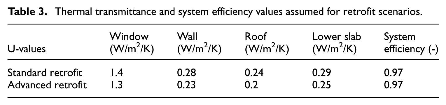
Thermal transmittance values and system efficiencies for each retrofit scenario (as detailed in Table 3) were defined based on the period of construction of the building. Two levels of intervention were modeled for the retrofit scenarios: minimum required standard practices (Anit, 2023) and advanced practices aligned with the Super bonus initiative (Ministro dello Sviluppo Economico, 2020). A total of nine scenarios were evaluated in this study, including the baseline, as well as window replacement, wall insulation, roof insulation, and global retrofitting, each examined at both standard and advanced levels. These scenarios were used to analyze energy consumption patterns and assess the Energy Poverty Index (EPI) under varying retrofit conditions.
Thermal transmittance and system efficiency values assumed for retrofit scenarios.
Calibration accuracy was assessed using a residual analysis comparing cumulative measured and simulated consumption, with the Absolute Percentage Error (APE) below 5%. Once calibration was completed, the process-driven model was used to simulate the actual consumption and various building retrofit scenarios.
Following the completion of the hourly H consumption simulations with the process-driven model, this study further integrated Machine Learning (ML) techniques, namely Light Gradient Boosting Machine (LGBM), to enhance the predictive capability of the model across a wider range of buildings and to enable rapid estimation under different retrofit scenarios. LGBM is a decision tree-based ML method that builds trees sequentially, correcting errors at each step. Its leaf-wise growth strategy allows for fast convergence, making it more efficient for regression tasks. These characteristics make it suitable for predicting building energy consumption where the data volume is large and features exhibit strong nonlinearity at an urban scale.
The model inputs included three categories of features: static building characteristics, dynamic weather conditions, and temporal variables. Building characteristics mainly include building volume, external wall area, window-to-wall ratio, thermal parameters (such as U-values of building components), construction year, and H system efficiency. Weather conditions cover hourly air temperature, solar irradiation, wind speed, and wind direction. Lagged variables were introduced to simulate the short-term inertia effects of climatic conditions on energy consumption. Temporal variables include hour codes, day of the week, holiday indicators, and the H system’s active period to reflect the impact of changes in residents’ behavioral patterns on energy use.
To ensure the predictive performance of the ML model, the dataset is split by building ID, and the Optuna optimizer with integrated cross-validation was used to tune the hyperparameters, thereby avoiding information leakage. The ratio of training to testing data is set to 80% and 20%, respectively. All models shared the same input features, with adjustments made only to variables related to building components’ thermal transmittances according to each retrofit assumption. The model is scenario-adaptive, capable of simulating the impact of different retrofit strategies on building energy performance (measuring the energy intensity in kWh/m3/y). This study independently modeled and optimized nine energy consumption scenarios to verify the predictive stability and generalization ability of the LGBM in different building renovation scenarios, allowing rapid scenario evaluation to assess energy-saving effects, investment costs, and changes in energy poverty.
E consumption in this study was estimated using the average residential user profile, while DHW was calculated according to the Italian standard UNITS 11300-2:2019.
The cost-optimal analysis was conducted using the global-cost equation (equation (1)) (Becchio et al., 2016) to assess the economic feasibility of retrofit scenarios.

CI is the initial investment cost [€]
Ca,i is the cost for year i, related to the component j (operation and management costs, running costs, substitution costs) [€]
Rd(i) is the discount factor for year i [-] (i.e. 0.03)
Vf,i(j) is the residual value of the component j at time i, [€].
For the energy poverty evaluation 10% indicator and the LIHC indicator, equations (2) and (3) were applied, respectively:


Ii is annual disposable household income [€]
Hi is the rent or mortgage payments [€]
hi is the fair rent increase according to building renovations [€]
Ei is the total household expenditure on energy services [€]
Cinvst,A is the annuitized investment cost [€]
Ti is the Municipal Property Tax (imposta municipale unica (IMU) in Italian) [€]
PLi is the relative poverty line equal to 60% of the median national household income [€]
To be able to effectively calculate the EPI in the subsequent years after the renovation, the annuitized investment cost is calculated using the Capital Recovery Factor (CRF) over 10 years, which is the period during which investors in building renovation are entitled to receive the tax deduction. The CRF is applied only to the advanced retrofit scenarios, where investors benefit from financial incentives through tax deductions. In contrast, for the standard retrofit scenarios, the global cost is not annuitized, as the full renovation cost is assumed to be paid in the initial year. The CRF is calculated using equation (4).

where n is the number of annuities received, and i is the interest rate.
For the fair rent increase as a result of the building renovations, it is assumed that for buildings built before 1960, the rent increase is equal to 8% of the investment cost, while for buildings built after that period, this rate is 5% of the investment cost (Ahlrichs and Rockstuhl, 2022).
QGIS-based solar irradiance simulator
Accurate information on local solar radiation is crucial for a wide range of applications, including architectural design and solar energy systems, as well as for design-oriented methods (Sarr et al., 2020). One of the primary domains of solar radiation analysis lies in the field of building physics, where solar radiation plays a fundamental role in governing heat transfer through the building envelope, influencing indoor thermal comfort, heating and cooling energy demand, and the overall energy performance of buildings. Most recent tools for solar radiation analysis rely on detailed 3D building models, which are not easily accessible or producible by all users, and typically involve high computational costs that limit their applicability in large-scale or data-constrained contexts.
One of the main aims of this work was to develop a QGIS-based solar irradiation simulator capable of analyzing solar radiation incident on each building component using the 3D information of the built environment. However, the same methodology can be applied using a 2.5D built environment that consists of building footprint, height information, and the geographic coordinates of the area of interest; these are the minimum requirements to apply this methodology across different urban contexts with varying morphologies.
This simulator is governed by the solar geometry formulation prescribed in EN ISO 52010-1 (2017). The position of the sun is computed on an hourly basis using astronomical relationships that define solar altitude and azimuth angles as functions of geographic latitude, longitude, day of the year, and solar time. These parameters are used to determine the direction of incident solar radiation for each time step. Based on the calculated sun position, shadow-casting effects between buildings are evaluated to account for mutual shading in the urban context. Finally, the angular relationships between the sun and building surfaces are used to determine the contributions of direct, diffuse, and reflected solar irradiance to both vertical and horizontal envelope components within the simulation framework. In the following, the equations strictly required to reproduce the solar geometry and shading logic are reported; the full theoretical background is available in EN ISO 52010-1: 2017.
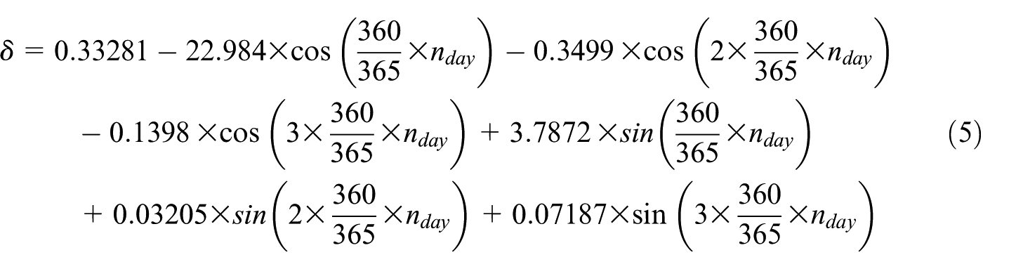
The solar declination, δ, in degrees, is determined by equation (5):
where
The solar hour angle,

when

where
TZ is the time zone, the actual (clock) time for the location compared to UTC (Universal Time Coordinated);
The solar altitude angle,

When

The solar zenith angle,

Where
The solar azimuth angle,
When

Where
The azimuth angles range between −180° and +180°; this is needed to determine which shading objects are in the direction of the sun. For detailed calculation of the auxiliary variables, refer to the EN ISO 52010-1: 2017.
The solar angle of incidence,

Where
According to equation (10), the calculation of solar incidence on building envelope components requires explicit knowledge of the tilt and orientation angles of each surface. Since this information is not directly available from 2.5D building footprint data, a QGIS-based spatial analysis workflow was developed to derive the required geometric parameters at the urban scale. Figure 2 illustrates the general workflow for the calculation of the vertical walls’ azimuth angle, knowing that the tilt angle is 90°.
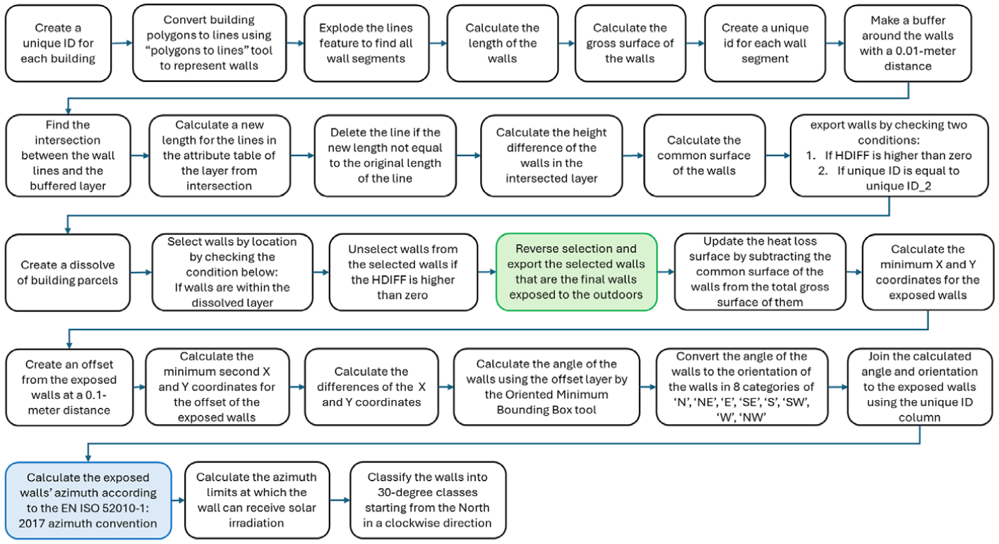
The QGIS steps to find the sun-exposed walls and their azimuth angle.
In this workflow, each building polygon is first assigned a unique identifier and converted into line features representing building walls, which are then exploded so that each wall segment is treated independently. The geometric properties of each wall, including length and gross surface area, are calculated, and a buffer of 0.1 m is generated around the walls to identify potential intersections with surrounding buildings. Spatial intersection analysis is then performed to detect obstructed wall segments, and height differences between the emitting and intersecting buildings are computed to quantify shading conditions.
Based on these intersections, common surface areas are calculated and subtracted from the gross wall surfaces to determine the effective exposed areas, while fully obstructed walls are excluded from further analysis. To calculate wall orientation, a geometric offset is applied to the exposed walls, after which the minimum X and Y coordinates are calculated for both the original wall and offset features, which are used to derive directional vectors. Wall orientation is then determined using the minimum oriented bounding box method, and the corresponding azimuth angles are calculated and constrained within the valid solar exposure limits defined by EN ISO 52010. For the horizontal or tilted roof surfaces, the workflow for calculating their slope and aspect is explained by Usta et al. (2025).
It is important to emphasize that treating all vertical and horizontal building components as distinct elements, each characterized by its own azimuth and tilt angle, allows the solar irradiation analysis to be performed individually for each surface, thereby ensuring a more accurate and reliable assessment of solar incidence on building envelope components.
Equation (11) expresses the global solar irradiance on a horizontal surface as the sum of its direct and diffuse components. The direct (beam) solar irradiance,

Where
The direct solar irradiance on an inclined surface,

Where
The diffuse component of solar irradiance on the surface, excluding ground-reflected contributions,

Where
SVF is the Sky View Factor of the inclined surfaces.
The ground-reflected contribution to the solar irradiance incident on an inclined surface,

When
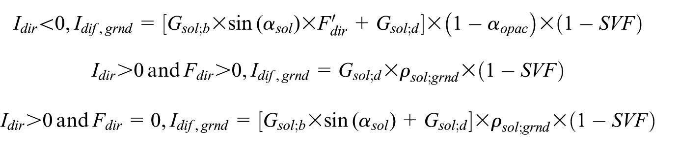
Where
SVF is the Sky View Factor of the inclined surfaces.
To account for solar radiation reflection in urban canyons, the reflected component of solar irradiance is corrected by considering three main interaction cases, as shown in Figure 3. When a building façade directly faces the sun, only the radiation reflected from the ground is considered. In this situation, if the street surface is not directly illuminated, the reflected radiation is assumed to come only from diffuse solar radiation reaching the ground. If the street surface is exposed to direct sunlight, both direct and diffuse radiation contribute to the reflected component. In both cases, the reflected irradiance is corrected using the complement of the SVF to represent radiation coming from surrounding urban surfaces. A third reflection case occurs when the building surface is not oriented toward the sun. This situation is considered only when the solar direction is nearly perpendicular to the surface, within a ±15° tolerance. In this case, solar radiation is assumed to be diffusely reflected between urban surfaces, first reaching the ground or nearby objects and then being reflected toward the receiving building surface.
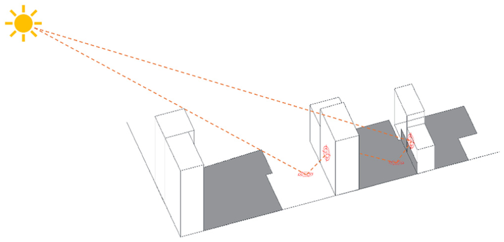
Representation of solar radiation reflection mechanisms in urban canyons.
The total solar irradiance on an inclined surface,

Where
To account for shadowing effects on building envelope components, a shading coefficient is calculated. This coefficient is defined as a geometric ratio between the height of neighboring buildings and their distance from the target building surface. The calculation is performed individually for each wall segment, ensuring that local variations in building height, spacing, and orientation are explicitly captured.
As illustrated in Figure 4(a), the shading assessment is based on the comparison between the solar ray path and the obstruction angle generated by surrounding buildings. A wall segment is considered shaded when the vertical obstruction angle, derived from the Height-to-Width (H/W) ratio of an adjacent object, exceeds the solar altitude angle for a given sun position. To further improve consistency with solar geometry conventions, the shading analysis is performed by classifying the solar azimuth into 30° sectors, as shown in Figure 4(b). For each wall segment, shading conditions are evaluated within each azimuth sector, taking into account the directional dependence of shadow casting.
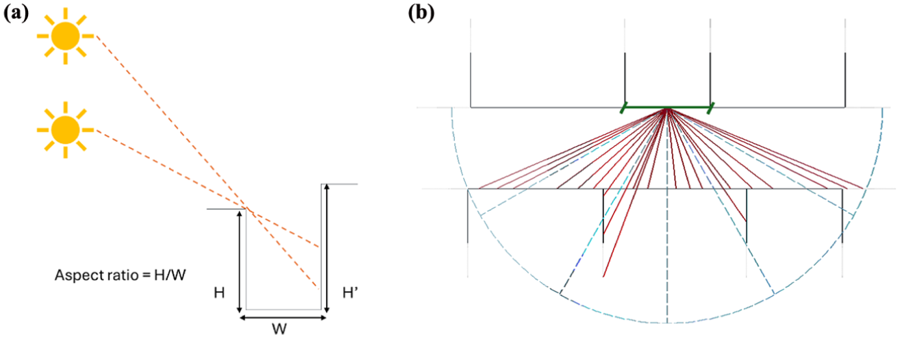
Illustration of the (a) shading coefficient calculation using H/W ratios, within (b) each sun azimuth sectors.
The H/W ratio for building walls is calculated using a QGIS-based analysis (shown in Figure 5) that identifies exposed wall segments and evaluates their surrounding urban context. For each wall, nearby objects, namely walls, are detected within a predefined search distance to identify potential shading obstacles, and the height difference between the wall and these surrounding elements is computed. The horizontal distance between the wall and the obstructing buildings is then used to calculate the H/W ratio. Wall orientations are derived and classified into 30° azimuth sectors according to EN ISO 52010 conventions. For each wall and azimuth class, the maximum H/W ratio is selected to represent the most restrictive shading condition affecting solar access.
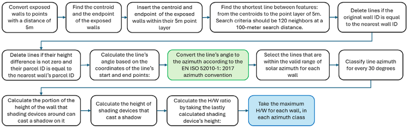
The QGIS steps to calculate the wall segment’s H/W ratio.
The H/W ratio for roof surfaces is also calculated similarly to the wall segments shown in Figure 6. Roof geometries are first segmented and classified by slope and aspect, after which surrounding roof elements are identified to determine height differences and distances. The maximum H/W ratio is then computed for each azimuth class.
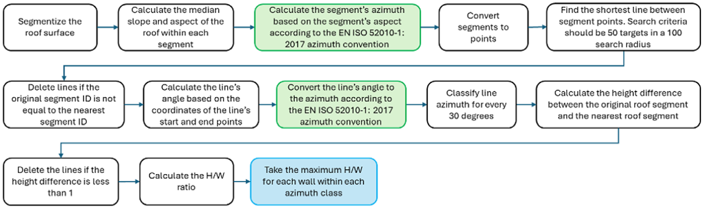
The QGIS steps to calculate the roof segment’s H/W ratio.
Results and discussion
This section presents the main findings of this study. Using a comprehensive dataset covering all relevant variables (about buildings, urban environment, climate conditions, inhabitants’ characteristics, and energy prices), both process-driven and ML models were applied to conduct a detailed analysis of the actual and future energy-consumption scenarios and their implications for energy poverty alleviation.
Solar irradiance simulator
To verify that the developed simulator achieves a level of accuracy suitable for integration within the physics-based UBEM framework, its outputs are validated against reference datasets. Specifically, simulated solar gains on horizontal surfaces are compared with measured solar radiation components recorded at the Politecnico di Torino weather station. In addition, solar gains on vertical building walls are independently evaluated through a comparative analysis with results generated by CitySim Pro, allowing the performance of the simulator to be assessed for both horizontal and vertical envelope components.
The comparison between measured and simulated solar radiation on the roof, Figure 7, shows a good overall agreement, confirming that the proposed simulator performs reliably for horizontal surfaces. The simulated direct solar irradiance closely matches the measured data throughout the year, with Mean Absolute Percentage Error (MAPE) about 2%. This indicates that the model correctly represents solar geometry and the projection of direct radiation on horizontal surfaces.
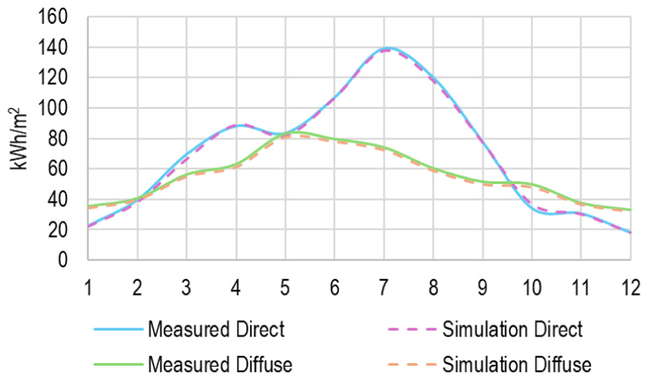
Comparison of measured and simulated direct and diffuse solar radiation on a horizontal surface.
For diffuse radiation, the simulation slightly underestimates the measured values during periods of high solar altitude, which can be attributed to simplified assumptions in the treatment of diffuse radiation and atmospheric scattering. Nevertheless, the MAPE remains low, at around 3%. Overall, these results show that the simulator can adequately reproduce direct and diffuse solar gains on roofs.
Figure 8 shows the wall segments used to compare the solar irradiance results from the developed simulator and CitySim Pro. Two different buildings are selected to represent different urban conditions. One building is located in a dense urban area, where the wall is affected by shading from surrounding buildings, while the other building has a south-facing wall that is largely free from shadows. This comparison helps evaluate the simulator’s performance under both shaded and well-exposed conditions.
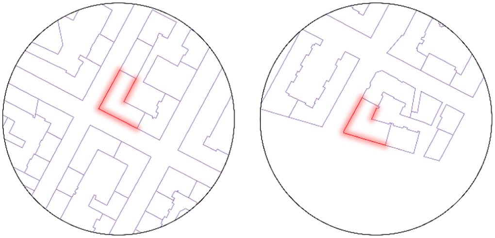
Selected wall segments used for solar irradiance comparison under shaded and unshaded conditions.
Graphs a, c, and e in Figure 9 compare the solar irradiation calculated by the proposed simulator with those from CitySim Pro and PVGIS for West-, South-, and East-facing walls of a building whose South wall is not affected by shading. It is important to mention that PVGIS does not automatically consider the obstruction horizon of the surrounding shading elements. In this work, for each point analyzed, the obstruction horizon angles were calculated separately and imported; obviously, this analysis cannot be performed for all façade elements of each building at an urban scale.
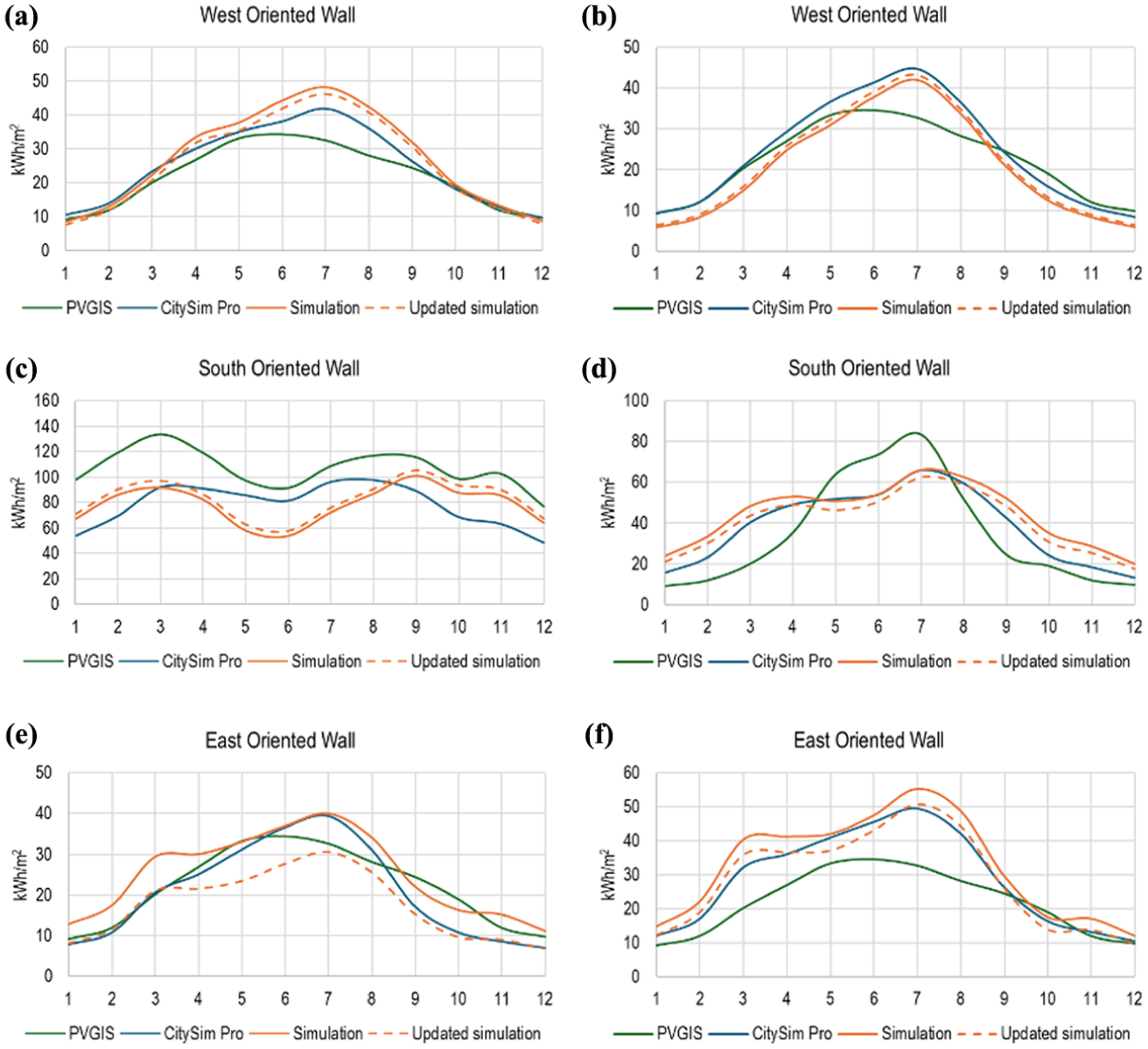
Solar irradiation on West-, South-, and East-oriented walls in a dense (a, c and e) and open (b, d and f) urban context.
In Figure 9, for the West-facing wall, the simulator captures the general seasonal trend but slightly overestimates the solar irradiation compared to CitySim Pro, leading to a MAPE of about 12%. The PVGIS results follow a similar seasonal pattern but remain consistently lower than both CitySim Pro and the simulator, particularly during summer months. For the South-facing wall, the agreement with CitySim Pro is weaker, with a MAPE of 23%. The simulator reproduces the main seasonal pattern and peaks reasonably well, although some differences remain, especially in summer. In this case, PVGIS consistently shows higher irradiation values in spring and late summer compared to both CitySim Pro and the simulator. However, the simulator and PVGIS exhibit a similar seasonal pattern for the South-oriented wall. This behavior is typical for obstruction-free South-facing vertical façades in mid-latitude climates and confirms that the geometric projection of solar radiation is correctly reproduced by the proposed simulator. The East-facing wall shows the largest difference compared to CitySim Pro, with a MAPE of 35%, where the simulator clearly overestimates the solar irradiation. PVGIS closely follows the CitySim Pro trend but generally shows lower magnitudes. Overall, the main source of error in the proposed simulator for all wall orientations is the estimation of the SVF, which affects the diffuse solar radiation. This effect is stronger for East- and West-facing walls, where diffuse radiation plays a larger role, and less important for the South-facing wall, which is mainly influenced by direct solar radiation.
The error in the SVF calculation mainly arises from a mismatch between the building boundaries shown in the Turin DSM and those in the corresponding buildings’ vector dataset. As a result of this mismatch, the assigned SVF values for wall segments may not accurately reflect their actual exposure conditions. A potential solution to minimize this source of error in the walls’ SVF assessment is to generate a 2.5D DSM raster directly from the buildings’ vector layer and then perform the SVF calculation using this locally generated dataset, ensuring geometric consistency between inputs. The use of 2.5D DSM also allows the replicability of this methodology in any city.
By correcting the mismatch between the SVF raster based on the 2.5D DSM raster generated from the building’s vector layer and the building wall segments, the MAPE between the results of the solar simulator and those from CitySim Pro recovered, bringing the curves into close alignment. The MAPE after correction becomes 11% and 12% for West- and East-oriented walls, respectively. However, for the South-oriented wall, the MAPE remained consistent, indicating that the residual error is not primarily due to geometric mismatch but rather to direct solar radiation prediction, since this wall segment is free from shading obstruction and direct solar radiation dominates.
Graphs b, d, and f in Figure 9 compare the simulated solar irradiation with CitySim Pro and PVGIS for West-, South-, and East-facing walls of a building in a dense urban area. For the West-facing wall, the simulator follows the seasonal trend but underestimates the solar irradiation, with a MAPE of about 20% compared to CitySim Pro. PVGIS values are generally lower than CitySim Pro, particularly during summer months. For the South-facing wall, the results show a slightly higher MAPE of 26% with respect to CitySim Pro. However, PVGIS exhibits a noticeably different seasonal pattern, with a sharper peak in summer and lower values in winter compared to both CitySim Pro and the simulator. For the East-facing wall, the simulator overestimates solar irradiation compared to CitySim Pro, leading to a MAPE of around 16%. In this case, PVGIS results are significantly lower than both CitySim Pro and the simulator, especially in spring and summer. In these three cases, the correction of the SVF was applied similarly. After correcting the SVF inconsistency, the agreement improves, and the MAPE decreases to 16%, 17%, and 6% for West-, South-, and East-facing walls, respectively. According to observed improvements, even in the dense urban case, the South façade continues to present the greatest discrepancies, mainly influenced by direct solar radiation. Therefore, although SVF correction reduces part of the discrepancy, the remaining gap is likely associated with differences in sky modeling and direct component treatment rather than geometric obstruction alone. Overall, the simulator shows reliable performance for urban-scale use. It reproduces the main seasonal patterns of solar irradiation on roofs and walls.
Space heating consumption
The H consumption for various scenarios, including baseline and retrofit scenarios, is simulated with a calibrated process-driven model. The data on energy consumption for H considers the heating season from November 2022 to April 2023. To evaluate the calibrated models’ performance, the results of the models were compared with measured data using the APE. In Figure 10, the results of three residential buildings with similar geometric characteristics but different construction periods were represented: B1 (1946–1960), B2 (1961–1970), and B3 (1991–2000).
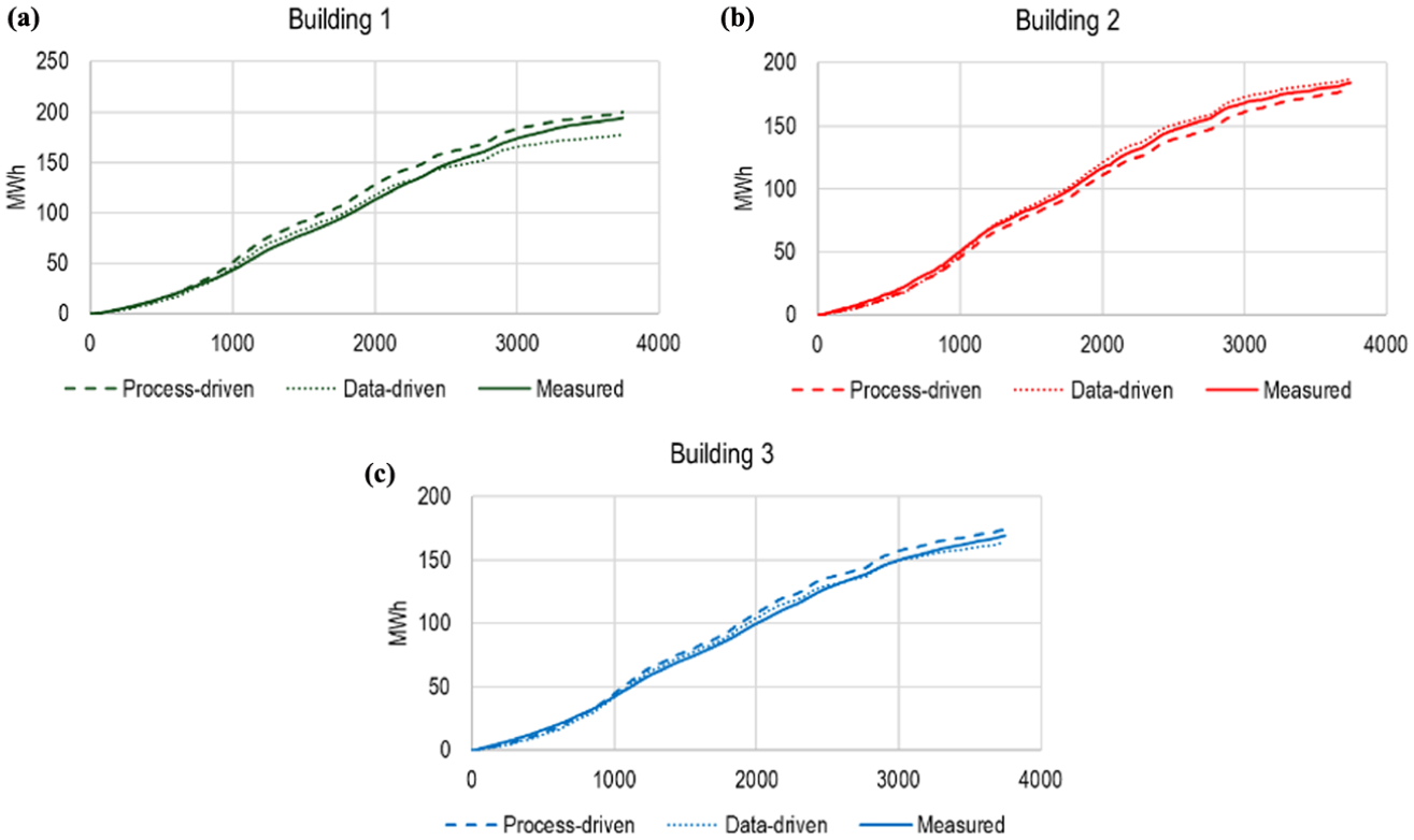
Cumulative energy consumption curves for H for similar buildings: B1 (1946–1960), B2 (19 61–1970), and B3 (1991–2000).
The cumulative energy consumption curves serve as a key indicator for evaluating both the calibration accuracy and overall performance of the UBEMs, particularly the process-driven model. These curves demonstrate that the process-driven model aligns closely with the measured energy consumption data, effectively capturing real-world consumption patterns. Notably, the APE for the process-driven model remains consistently below 5%, confirming the model’s robustness. This high level of accuracy underscores its reliability in simulating energy efficiency strategies and in quantifying the effects of different retrofit scenarios, particularly for assessing their implications on energy poverty at the urban scale.
Model optimization with LGBM ML model
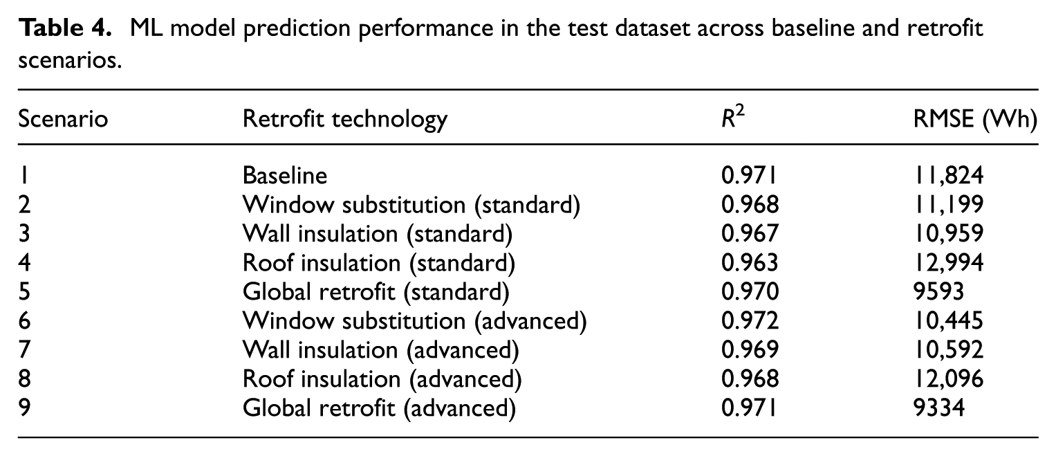
Table 4 and Figure 11 show the performance of the ML model utilized in this work compared to the process-driven UBEM simulation results. Overall, LGBM demonstrated high accuracy and consistent performance across most scenarios. The baseline scenario showed stable results, achieving an R2 of 0.971 and an Root Mean Squared Error (RMSE) of 11,824 Wh, on the test set, providing a benchmark for evaluating the other retrofitted scenarios.
ML model prediction performance in the test dataset across baseline and retrofit scenarios.
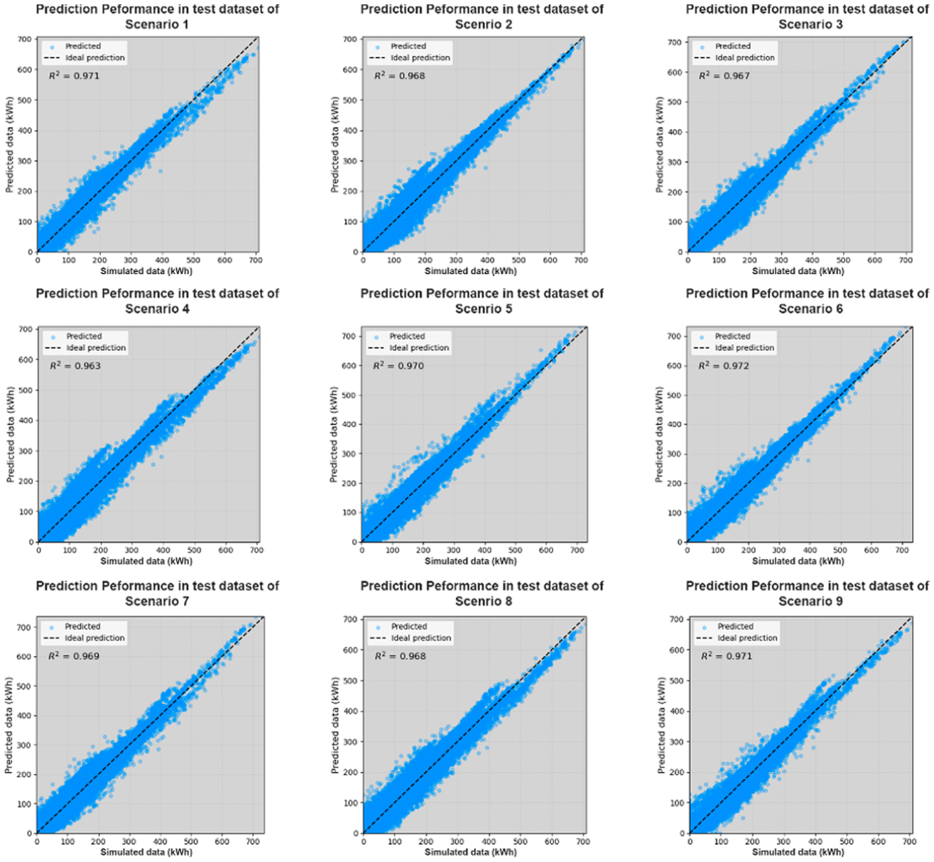
LGBM ML predicted versus UBEM simulated heating consumption in the test dataset across the nine analyzed scenarios.
As building heat loss decreased, models under standard retrofit scenarios still maintained stable prediction accuracy. Although R2 slightly declined (ranging between 0.963 and 0.970), RMSE showed downward trends, indicating that the reduced energy demand also led to lower absolute errors. For example, in the windows insulation scenario, with RMSE reduced to 11,199 Wh. These results suggest that the ML model retains strong generalizability even under retrofit interventions. In the advanced retrofit scenarios, an increase in R2 and a drop in EMSE were observed compared to the standard scenarios. This indicates that the predictive accuracy of the model for advanced retrofit scenarios was improved, and more stable model performance was observed, particularly for window substitution and global retrofit cases.
Figure 12 illustrates the cumulative energy consumption curves of a sample building to check the accuracy of the predictions. For instance, the cumulative curve under the baseline scenario exhibits a steady increase, with ML model predictions closely aligned with the UBEM simulation results until mid-season, where a slight underestimation has been observed. In contrast, under retrofit scenarios, the predicted curves become more aligned with the simulation curves, except in global retrofit. This difference comes from how different the buildings become after each retrofit. In single retrofit cases, only one building feature is changed, so buildings still differ, and the model can better capture variations in energy use. In global retrofit cases, all buildings are upgraded in the same way, making their heating demand very similar. Because of this reduced variation, the model struggles to distinguish between buildings, which leads to underestimation and higher annual errors.
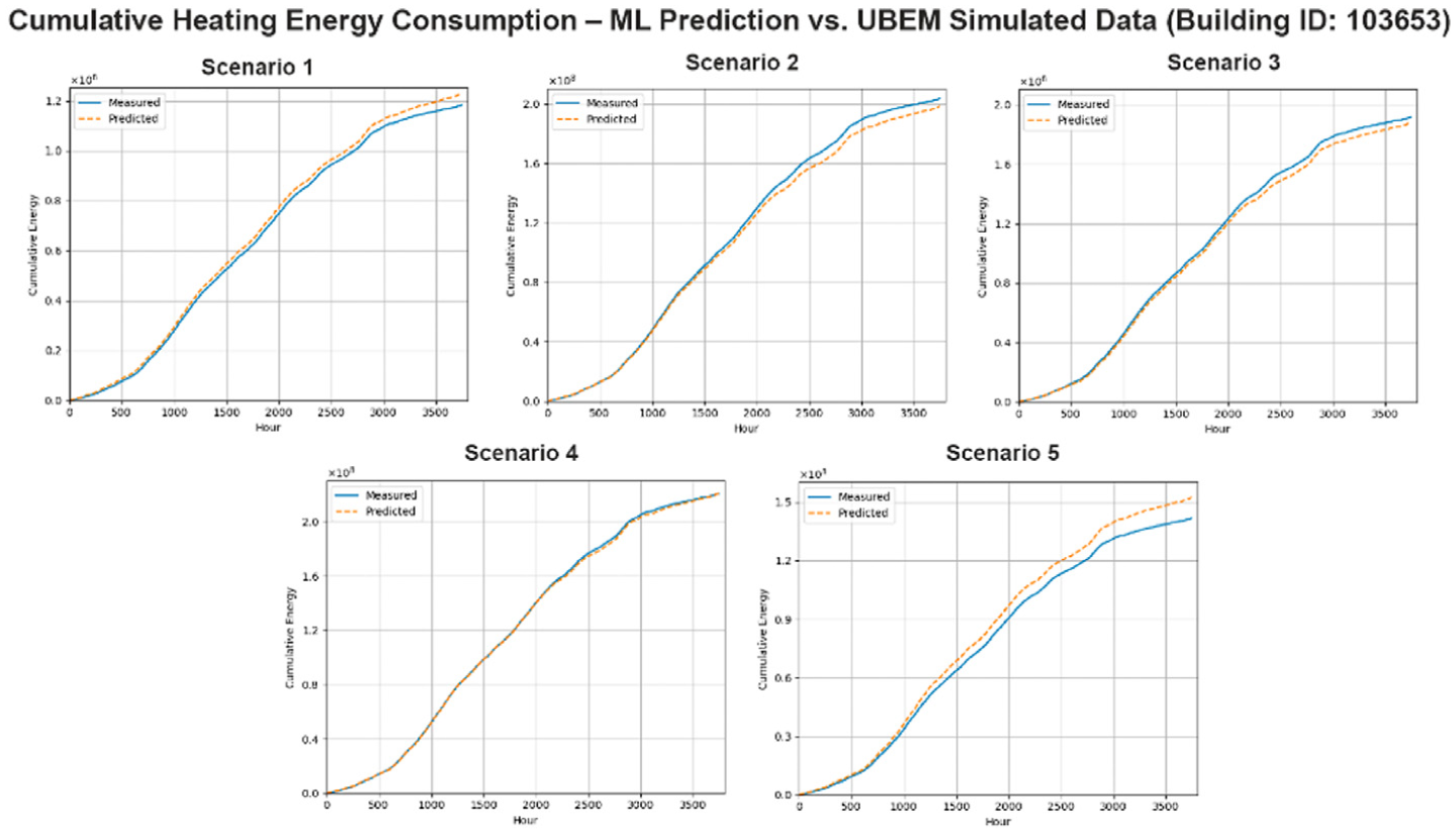
Cumulative heating consumption profiles for a representative building: LGBM ML predicted versus UBEM simulated results for baseline and standard retrofit scenarios.
To better understand how the ML models behave under different scenarios, this study carried out a systematic analysis of feature importance for each trained LGBM model. Figure 13 presents the top 20 most influential features for the baseline and the eight retrofit scenarios, ranked according to their importance in the baseline case, and shows how the model’s reliance on different input variables changes as the thermal characteristics of buildings are modified.
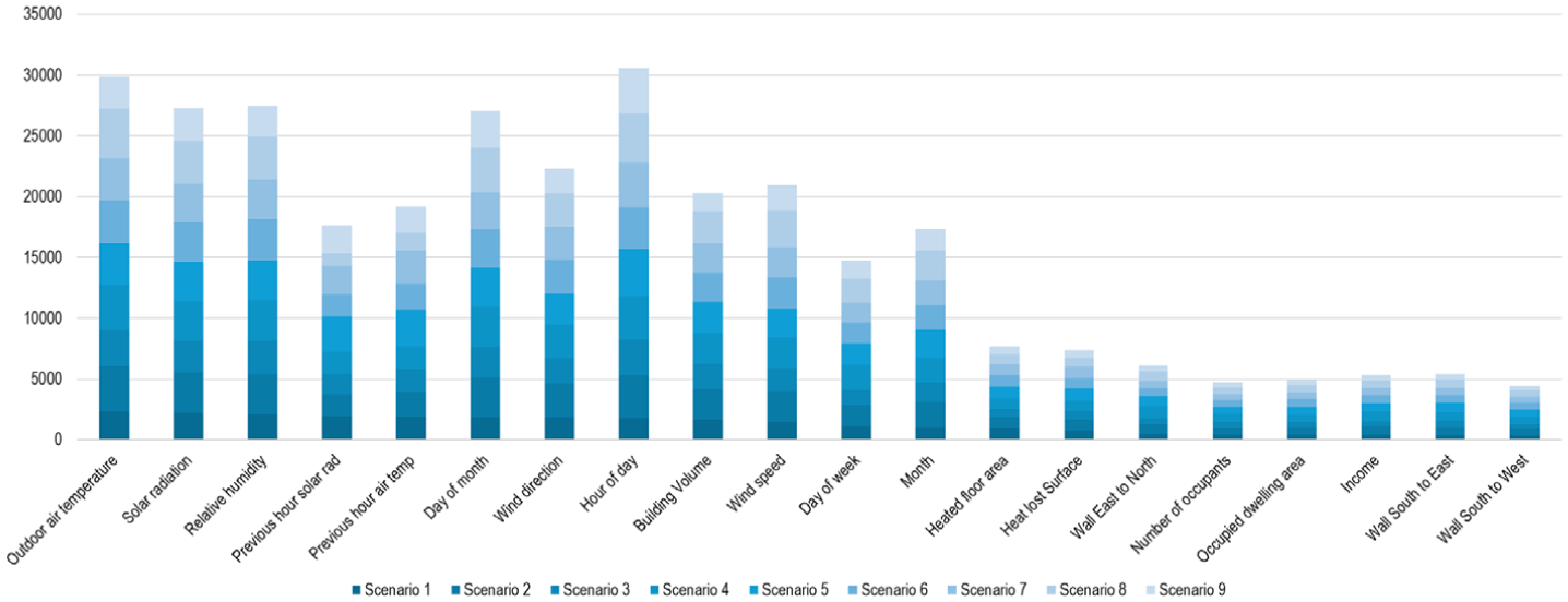
Top 20 most influential energy-related features in the heating consumption prediction model across scenarios.
In the baseline scenario, climatic variables and building characteristics have the strongest influence on the model predictions. Average outdoor temperature, solar radiation, and outdoor relative humidity are the most important inputs, with values of 2350, 2188, and 2114, respectively, showing that hourly heating demand is highly affected by external climate conditions. Variables from previous hours, such as lagged temperature and solar radiation, are also important, indicating that the model captures the effect of building thermal inertia over time. Among building features, volume, surface-to-volume ratio, number of floors, and construction period contribute noticeably to the predictions. In contrast, thermal performance parameters such as wall and roof U-values have very low importance, mainly because they are assigned by construction period groups and therefore do not strongly differentiate buildings in the baseline scenario.
In all retrofit scenarios, whether at standard or advanced levels, the importance of input features changes noticeably. Because the U-values of the retrofitted components are set to the same value for all buildings, this variable no longer helps the model distinguish between different cases. For instance, in the standard window retrofit scenario, the importance of the glazing U-value drops to zero.
As a result, the model relies on other parameters, in particular, more on climatic variables, such as average outdoor temperature and solar radiation, making them the most influential inputs. At the same time, other factors such as building volume, building occupancy, and population become relatively more important and act as secondary predictors.
Economic and social analysis
This study included a cost-optimal analysis to assess the economic and social feasibility of different retrofit measures. Global costs were calculated at the building level and then normalized per household. Annuitized investment costs were analyzed by construction period to identify the most cost-effective retrofit option for each building category.
Buildings constructed after 2005 were excluded from the analysis because of the limited availability of consumption data for model training and because these buildings are assumed to comply with more recent energy performance standards, making retrofit interventions less necessary.
Table 5 presents a detailed breakdown of the cost-optimal analysis for the retrofit scenarios by construction period. Among the evaluated options, wall insulation emerges as the most economically feasible retrofit measure. It is also one of the most effective interventions in terms of energy performance. It provides a clear reduction in energy intensity while keeping global costs relatively low compared to window replacement and global retrofit measures. In several cases, especially in the advanced scenario, the global cost of wall insulation is close to or even lower than the baseline, confirming its cost-effectiveness. Window replacement reduces energy intensity but results in much higher global costs in the standard scenario, making it less attractive when implemented alone. Roof insulation shows moderate energy savings, but its economic advantage is generally smaller than that of wall insulation.
Energy Performance Intensity and global costs comparison across baseline and retrofit scenarios by period of construction.
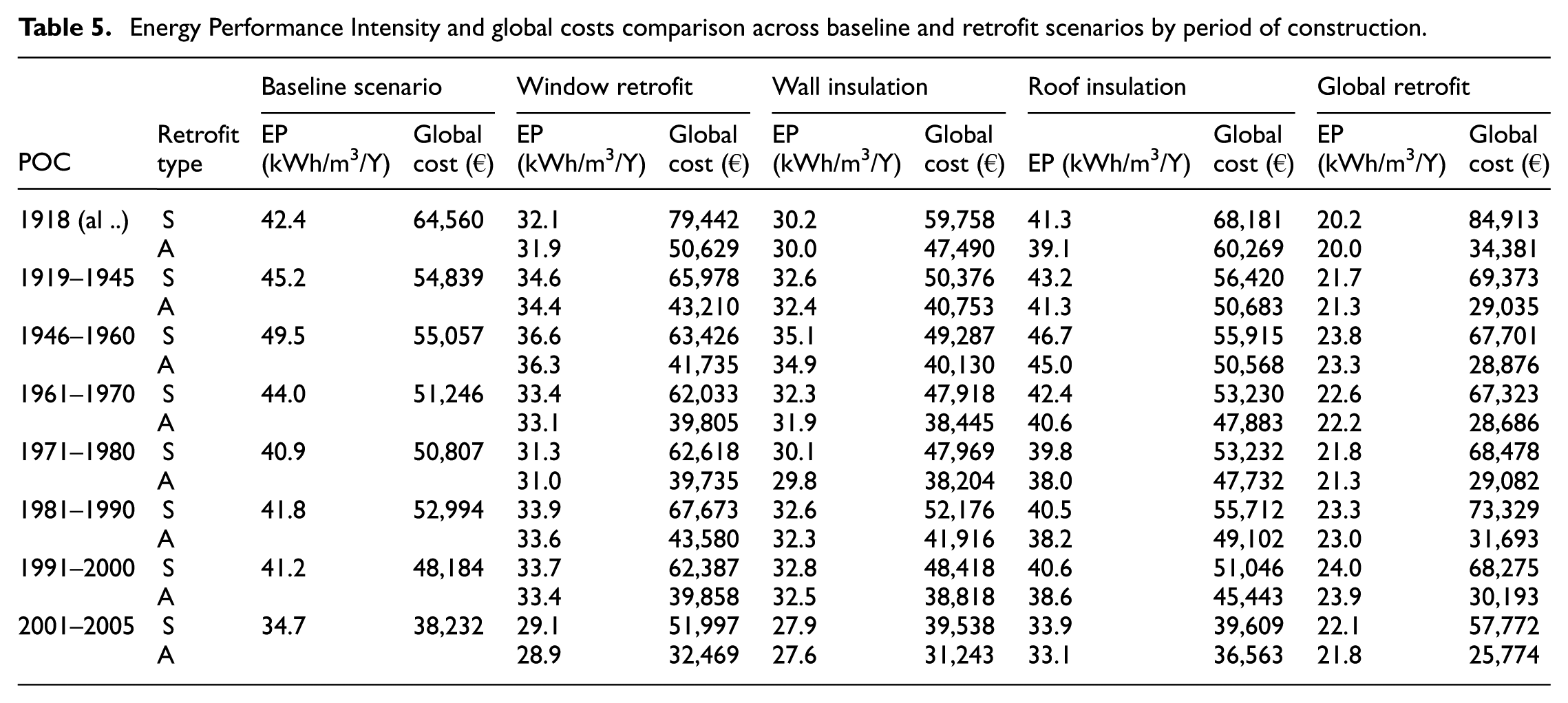
Furthermore, the results indicate that advanced retrofit strategies can become financially viable when combined with tax incentives available under the Super bonus scheme. These incentives substantially improve the economic feasibility of global renovation interventions, making them the most attractive option for long-term energy upgrading. It should be noted, however, that the Super bonus does not involve direct public funding. Instead, households can recover up to 65% of the eligible investment costs over several years through income tax deductions, provided that the retrofit measures comply with the energy performance requirements established by the regulation, including prescribed U-value thresholds.
In line with the EPAH guidelines (Energy Poverty Advisory Hub, 2024), this study applied two widely used indicators to assess energy poverty in the city of Turin: the 10% income threshold and the LIHC indicator. The analysis considered not only renters, who represent a large share of vulnerable households, but also homeowners, evaluating their potential risk of entering energy poverty after retrofit interventions. For renters, possible rent increases following renovations were taken into account to ensure a fair assessment of post-retrofit affordability. For homeowners, the cost of renovation was evaluated in relation to the available tax deductions. In all cases, changes in household energy expenses across the different retrofit scenarios were consistently included in the energy poverty assessment.
Figure 14 presents the results of the EPI assessment for the baseline scenario and all retrofit measures. The results show that energy poverty levels change significantly depending on the retrofit scenario and the indicator used. Under the baseline conditions for the 2022–2023 period, energy poverty in Turin ranges from about 14.4% according to the LIHC indicator to 17.6% based on the 10% threshold. In the standard retrofit scenarios, where no incentive is provided to investors in renovation costs, the effects are mixed. Wall insulation slightly reduces energy poverty (16.5% under the 10% threshold and 6.3% under LIHC), while roof insulation has only a small impact (17.8% and 12.4%, respectively). However, window replacement increases energy poverty under the 10% threshold (30.4%), and the global standard retrofit raises it even further (32.8%). This happens because the 10% indicator is very sensitive to high initial renovation costs. In contrast, the LIHC indicator shows a reduction in all standard scenarios. This is mainly because LIHC is based on a double threshold: households must meet both the high-cost and low-income conditions at the same time. When energy performance improves after a retrofit, at least one of these conditions is often no longer satisfied, which leads to a decrease in the measured energy poverty rate.
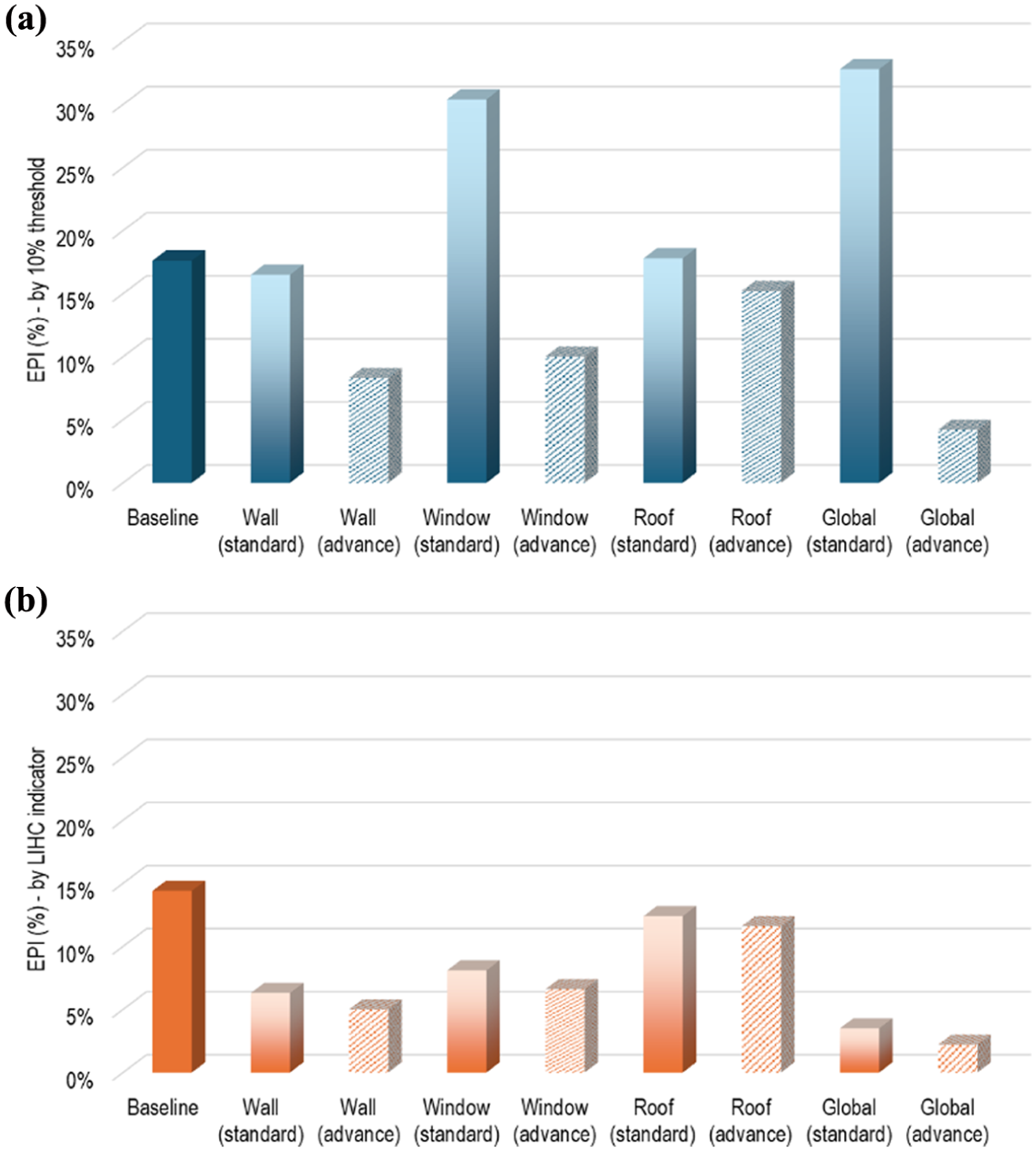
Energy poverty index of the baseline and retrofit scenarios using the (a) 10% threshold and (b) LIHC indicator.
In the advanced scenarios, where renovation costs are spread over 10 years and supported by tax incentives, energy poverty decreases consistently under both indicators. The global advanced retrofit shows the greatest improvement, reducing energy poverty to 4.2% and 2.2% according to the 10% threshold and LIHC, respectively. These findings highlight that the financial structure of retrofit measures is crucial to guarantee their social impacts. Without incentives, deep renovations may increase financial pressure on households, while well-designed support schemes can effectively reduce energy poverty. Moreover, for EPI assessment, the LIHC indicator can offer a more comprehensive evaluation of energy poverty compared to the 10% threshold, as it accounts for both affordability and income vulnerability rather than relying solely on energy expenditure shares, and it is widely recommended by institutional and policy organizations for official assessments.
Regarding the spatial distribution of the EPI for the baseline scenario across postal code zones (Figure 15(a), based on the LIHC indicator), central and hillside areas show relatively low levels of energy poverty, while higher values are mainly concentrated in the northern peripheral districts, particularly in postal code zones 10156, 10154, 10151, 10155, and 10122.
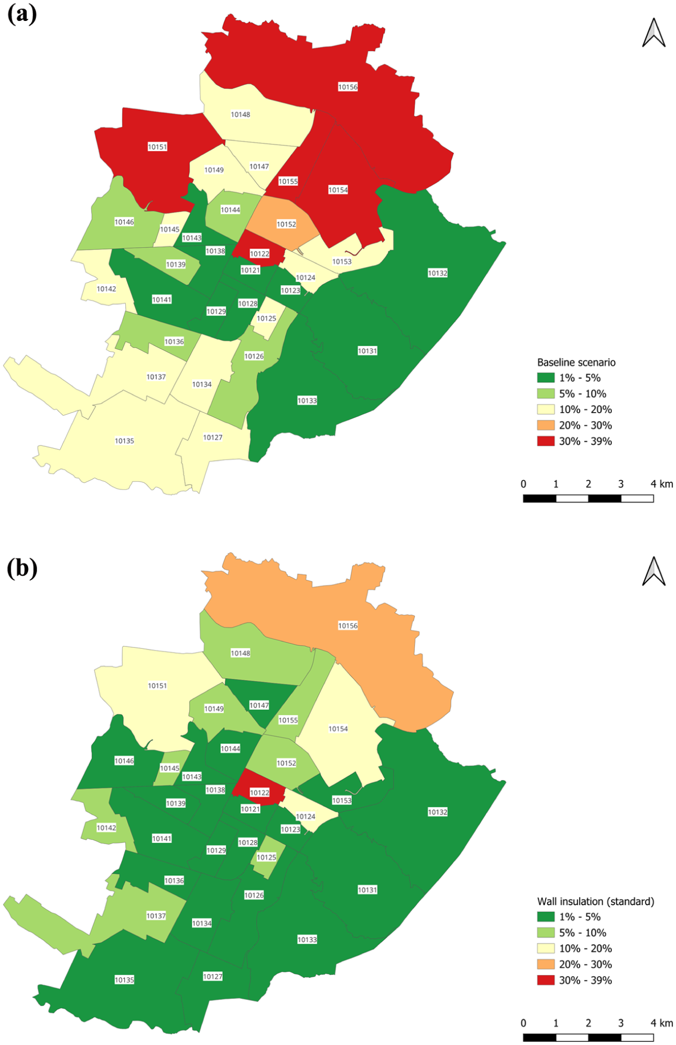
EPI visualization of (a) baseline and (b) standard wall insulation scenarios.
Wall insulation (Figure 15(b)), identified as the most effective single intervention under the standard renovation strategy, leads to more widespread benefits, reducing energy poverty below 15% in almost all areas. Nevertheless, zones 10156 and 10122 continue to stand out as a critical area, with energy poverty levels still exceeding 20%, indicating persistent vulnerability even after retrofit measures.
It is important to note that these results are based on an ideal scenario in which all buildings are retrofitted at the same time. In reality, this is not feasible due to structural, logistical, and financial limitations. Historical data show that only about 2% of buildings are renovated each year (Mutani and Todeschi, 2021), which significantly slows down the potential impact on energy poverty reduction. Therefore, while the results demonstrate the effectiveness of retrofit strategies, they also highlight the need for targeted, long-term policies that focus on the most vulnerable households and support a gradual and equitable transition.
Conclusion
The solar gain assessment developed in this study proved to be a robust and computationally efficient method for improving the representation of boundary conditions in urban-scale energy modeling. The proposed QGIS-based simulator successfully estimates solar gains on both horizontal and vertical building components using 2.5D building footprints enriched with height and orientation information, while accounting for urban shading effects through simplified geometric relationships and SVF estimation. Validation against measured data shows very good agreement for horizontal surfaces, with a MAPE of approximately 2% for direct radiation and 3% for diffuse radiation. For vertical façades, comparison with CitySim Pro indicates that before correcting the SVF inconsistency, the MAPE ranged between 12% and 20% for West-facing walls, 23%–26% for South-oriented walls, and up to 16%–35% for East-facing walls, depending on the urban density. After ensuring geometric consistency between the DSM and vector datasets, the errors were significantly reduced to approximately 11%–16% for West-facing walls and 6%–12% for East-facing walls, confirming that SVF estimation was the dominant source of error for diffuse-dominated orientations. In contrast, the error for the obstruction-free South façade remained around 23%, indicating that the residual discrepancy is primarily related to direct solar radiation prediction rather than geometric shading effects.
The study evaluated a range of retrofit scenarios, classified as standard and advanced, and assessed their economic feasibility based on investment costs and national tax incentive schemes. Wall insulation emerged as the most cost-effective intervention, particularly for buildings constructed before 1980. For these older buildings, energy intensity was reduced by up to 10.7 kWh/m3/year, while global renovation costs were significantly mitigated through available tax incentives.
In terms of energy poverty, assessed using both the 10% threshold and the LIHC indicator, baseline levels across Turin ranged from 14.4% to 17.6%. The implementation of the most effective retrofit measure, which is wall insulation, led to an average reduction of 8.1%, with energy poverty levels falling to as low as 6.3%. In an optimistic scenario, the implementation of a global retrofit, combined with tax incentives, can lower the EPI to approximately 2.2%. Spatial analysis further showed that vulnerable neighborhoods, particularly in the northern districts (e.g. 10154), experienced substantial improvements, with reductions of up to 35%. Nevertheless, some areas, such as postal code zones 10156 and 10122, remained critically affected even after retrofit interventions.
It must be emphasized that these results represent an idealized scenario in which all buildings are retrofitted simultaneously, which is not achievable under current renovation rates of approximately 2% of the building stock per year. This limitation underscores the need for targeted, long-term renovation policies that prioritize the most vulnerable households and support a gradual and equitable transition.
Overall, this study demonstrates that integrating high-resolution urban energy modeling with socio-economic indicators provides a solid foundation for designing just urban energy policies. The proposed methodology is scalable and replicable, offering valuable insights for municipal authorities, planners, and policymakers seeking to reduce urban energy poverty while promoting energy efficiency and social equity. However, this study assumed uniform climatic conditions and did not explicitly consider local microclimate effects, though they are highly important in urban-scale energy consumption analysis. For this reason, it is recommended that future research include these factors to further improve the accuracy of urban energy demand assessments across different retrofit scenarios and their potential in reducing EPI.
Footnotes
Acknowledgements

Ethical considerations
Ethical approval was not required for this study.
Funding
The authors received no financial support for the research, authorship, and/or publication of this article.
Declaration of conflicting interests
The authors declared the following potential conflicts of interest with respect to the research, authorship, and/or publication of this article: Ahad Montazeri reports that financial support was provided by the Ministero dell’universitá e della ricerca. If there are other authors, they declare that they have no known competing financial interests or personal relationships that could have appeared to influence the work reported in this paper.
Data availability statement
Data will be made available on request.*