Quantifying defensive performance in football: A piecewise parametric survival approach to goal scoring time

Abstract

To a significant extent, strategy deployment in sports has become data-driven. This has given rise to the application of data analytics in different sports, and football is no exception. This paper models the performance of selected national football teams, ranked among the highest in the FIFA standings as of June 2023, while playing against significantly lower-ranked opponents (minnows). When minnows play a relatively stronger team, their prime concern is not to concede a goal, thereby organising a deep defensive line, making it difficult for the more vigorous opposition to score. Thus, considering the time to the first goal scored by a stronger team as a time to an event, parametric survival analysis is applied in this study to compare the performance of stronger football teams against minnows. The study finds that the hazard function is neither a monotonic function nor a bathtub curve; instead, it takes a zig-zag form. This calls for a piecewise fitting of the survival distribution, which provides a better fit than any standard survival distribution proposed in the literature. By fitting such piecewise survival curves for each selected national side, one can identify sides that can better handle the minnows in football.

Keywords

FIFA rankings goal timing soccer sport analytics tactics

Introduction

With advances in computer technology, data collection, storage, retrieval and analysis have become more accessible than before. This has paved the way for the application of data analytics in almost every field of knowledge. Analytics is a growing field that utilises big data sets and analyses them with sophisticated analytical and visualisation tools to investigate, predict and assist in decision-making. Sports Data Analytics has become integral to all modern ball games. Football, the most popular sport on Earth, has seen an extensive application of such analytical tools. It is seen that the application of advanced analytics can lead to a significant impact on the strategies framed in professional football.¹ Machine learning tools are now regularly applied in professional sports to predict the outcome of matches, predict player injury, correct valuation of players, player analysis, performance prediction, etc.^2–4 In this paper, the researchers have tried to find out how long it takes for the stronger national football sides to score the first goal against their opponent, which is distinctly weaker. Smith⁵ opined that defensive compactness, time management and tactical adoption are a few strategies that weaker football teams adopt to restrict stronger sides from scoring. This paper applies parametric survival analysis to compare the performance of the six selected highest-ranked national teams (based on FIFA rankings as of 6^th June 2023) while playing against ominously weaker opponents. The study adopts a retrospective approach, analysing historical matches to evaluate how these currently high-ranking teams have performed and evolved over time against such opposition. Here, the stronger team's performance is quantified using the time to first goal, as the weaker opposing team generally builds a compact defence and restricts them from scoring. For this study, opponents ranked at least 30 places below the selected teams are classified as “minnows”. This threshold is supported by an examination of the last five FIFA World Cups (2006–2022), which show that teams ranked 30 or more places below their opponents have seldom reached the quarterfinal stage, highlighting the rarity of lower-ranked teams advancing deep in the major tournaments.⁶ Additionally, sports media frequently use the term “minnows” to describe teams ranked 30 or more places below stronger opponents, further reinforcing the use of this cutoff in football discourse.⁷

Literature review

Applications of analytical tools to address issues related to sports have gained momentum lately, especially with advances in computational technology. Along with academic research, the application of sports data analytics to improve team and individual players’ performance or decode strategies of opponents has become commonplace. Now, most players/teams, irrespective of the type of sport, have people with analytical expertise among their support staff. These professionals analyse the performance-related data of the concerned player (or team) and their opponents logically and diagnostically to improve performance or adjust strategy as appropriate.

Some research works provide a general overview of the application of data analytics in sports.^8–11 All these texts provide an excellent review of how modern-day sports are becoming more data-driven, citing examples from significant team and individual sports. Sports like baseball, cricket, etc., produce enormous data sets and player/match statistics. Such sports have found long-established statistical interventions. Numerous other sports have also developed their statistics, metrics and datasets and are now benefiting from analytics in sports decision-making, performance measurement and management.

Football has a professional research association called the Professional Football Researchers Association (PFRA) that publishes bi-monthly articles covering statistical analyses and new performance measurement methods.⁸ Though written with a different purpose, Drivet's work explains how different statistical tools can be better communicated to secondary school students using football data.¹² The work of Mackenzie and Cushion reviews existing literature relating to performance analysis in football. The authors further opined that alternative approaches to performance measures in football are necessary.¹³ One of the pioneering works of applying Markov Modelling in tactical decision-making in football was covered in the works of Hirotsu and Wright.¹⁴ Liu and Hohmann also applied Markov chains to study the performance relevance of passes in the 2011 European Champions League final between Manchester United and FC Barcelona. The paper identifies that player-to-player passes have a higher chance of taking the ball near the opponent team's goalpost.¹⁵ Continuous-time Markov chain models were used by Meyer et al. to accomplish statistical analysis of data generated from the Australian Football League. The attempt was to test certain assumptions of continuous-time Markov chain models for data coming from the tournament's different time, speed, and distance-related entities.¹⁶ Edmans et al. applied the econometric models to identify how eliminating national teams in high-profile international tournaments like the FIFA World Cup or the European Cup leads to a next-day abnormal stock return.¹⁷ Memmert and Raabe penned a complete book explaining the need for extensive data analysis and how modern data science and technology tools can help manage and develop individual players and teams.¹⁸

The tools utilised in survival analysis primarily pertain to the analysis of time to an event and have also found frequent application in football analytics. Nevo and Ritov applied the Cox proportional hazard model to determine the significant covariates that influence time to soccer's first and second goals and compared the two. The study finds that the chance of scoring the second goal increases once the first goal is scored.¹⁹ Rowson et al. used survival analysis to investigate the chance of temporary unconsciousness of individual football players following a collision and discussed some remedies to avoid such incidents.²⁰ Glasson and Bedford (2009) used survival analysis tools like hazard function and Cox-proportional hazard function to identify how the ranks of players while drafting affect the length of players’ careers in Australian football.²¹

An interesting aspect would be seeing how the national teams approach their matches against the minnows. In football and several other team games, it has been found that when a higher-ranked team plays a significantly weaker team, the match mostly becomes one-sided in favour of the stronger team. However, there are occasions when such matches turn out to be a war between “David and Goliath”- where the weaker team makes the way to victory difficult for their considerably stronger opponent. With a strategic approach, a weaker opponent can often disrupt the plan for the stronger teams in several ways. This can happen in any team sport, including football. Such disruption of the planning of stronger teams can be because of

using the services of their asset players to their full potential against a weaker opponent who could otherwise be fully or partially rested.

apply hidden strategies to overcome an ordinary challenger, which could otherwise be kept reserved for a more formidable opponent.

hamper or increase the difficulty level to progress to the next round in case of a tournament, and so on.

However, such an important issue was never addressed analytically in the case of any team sport, including football. No study covering this aspect has enriched our literature search. This sets the motivation behind the work. The attempt is to quantify how well a higher-ranked team can handle the challenges a relatively weaker opponent poses. Upon successfully completing this task, the methodology can be extrapolated to other sporting activities with distantly comparable opponents.

Statement of the problem

The research gap identified pertains to the quantification of ways in which a higher-ranked football team can negotiate the pressure exerted by weaker opponents. It is perceived in the case of football that defensive compactness, time management, and tactical adoption are a few strategies that weaker teams realise to restrict stronger sides from scoring. Once the stronger team scores the first goal, the defensive compactness of weaker teams shall also be lessened to a greater extent, as the latter will also come forward in search of goals. As the weaker teams restrict the high-ranked teams from scoring, the objective of the work is to quantify and compare the time taken by high-ranked teams to score the first goal against weaker opponents and hence take the lead. Only the time to the first goal scored by the higher-ranked team was considered as the event of interest. Matches in which the higher-ranked team failed to score were treated as right-censored, regardless of whether the lower-ranked team scored. The goal(s) by the weaker team were not considered part of the censoring mechanism, as the analysis was focused solely on the scoring performance of the stronger team.

A look into the performance of the selected six FIFA teams (ranked in the top six position as of 30^th June 2023) against considerably weaker teams (ranked at least 30 positions below on the date of the matches) can be seen in Table 1.

Table 1.

Performance of selected six national football sides against considerably weaker teams (matches selected from their last 250 international games).

FIFA ranking	Name	Time period	Total matches played	Matches considered for analysis (played against minnows)	Average time to first goal (mins.)	Average goal difference	Win percentage
1	Argentina	18/4/2007 to 20/11/2024	250	112	33.38	+1.79	72.32
2	France	17/08/2006 to 15/11/2024	250	97	34.80	+1.71	72.44
3	Brazil	02/07/2007 to 15/11/2024	250	93	30.76	+2.12	76.59
4	Belgium	11/06/2003 to 18/11/2024	250	92	33.05	+2.18	76.09
5	England	08/10/2005 to 17/11/2024	250	100	32.29	+2.45	81.18
6	Netherlands	08/06/2005 to 20/11/2024	250	100	30.58	+1.96	78.21

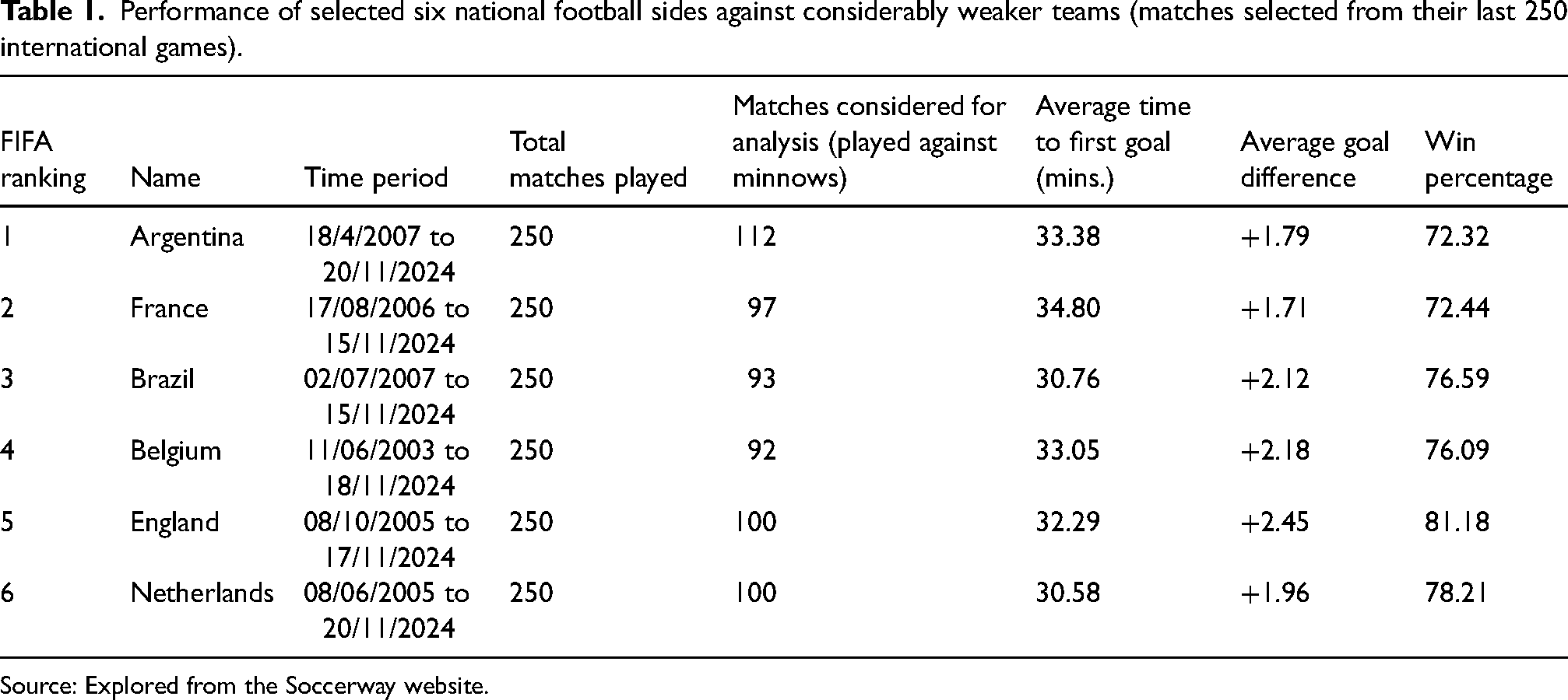
Source: Explored from the Soccerway website.

It is evident from Table 1 that though the elite teams are expected to get a victory against teams with a ranking at least 30 steps below, it is not always as easy as it is deemed to be. Most teams take 30 min (1/3^rd of the total time) or more to get their first goal against weaker opponents on aggregate. England is the most crushing against weaker opponents as they maintain a vast goal difference and have a higher percentage of victories. France has the lowest goal difference, + 1.71, compared to the other teams and has a win percentage just above Argentina. The table topper and the World Champions (2022), Argentina, have the lowest win percentage and find themselves in the most challenging situation when they attempt to overpower weaker opponents.

Objectives of the study

From the above discussion, one feels that the performance of these teams against weaker opponents requires a more intricate technical evaluation. Such evaluation shall open up the scope for more strategic planning on the approach of stronger teams against weaker competitors. On the other hand, such an exercise can also help build the weaker teams’ strategy to break the rhythm of stronger teams and restrict them from winning quickly and convincingly, making soccer matches more competitive.

More specifically, the following objectives are penned down:

To develop a methodology to quantify the time to the first goal by a stronger team against weaker opponents in football.

To compare the performance of the selected national football teams in terms of time to first goal against weaker opponents.

Methodology

Survival and hazard function

Survival analysis is a combination of statistical techniques where the outcome variable of interest is time until a given event occurs. In this case, it is the time for the first goal by a selected football team in a match against a minnow. One may consult Kleinbaum & Klein for details on survival analysis.²²

If T denotes the random variable representing the time to the first goal by a stronger football team while playing against a minnow, then S(t) gives the probability that the stronger team takes longer than some specific time t to score their first goal. In other words, S(t) gives the probability of survival of a minnow while playing against an elite national side without conceding the first goal. Thus,

S (t) = P (T \geq t)

(1)

The hazard function is defined as the instantaneous chance of scoring a goal by the higher-ranked national football team while playing against a minnow per unit of time, given that the former could not score by time t. In terms of probability, it is expressed as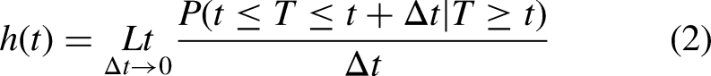

h (t) = \underset{Δ t \to 0}{L t} \frac{P (t \leq T \leq t + Δ t | T \geq t)}{Δ t}

(2)

So, the hazard function is not a probability function but a ratio.

Parametric survival analysis

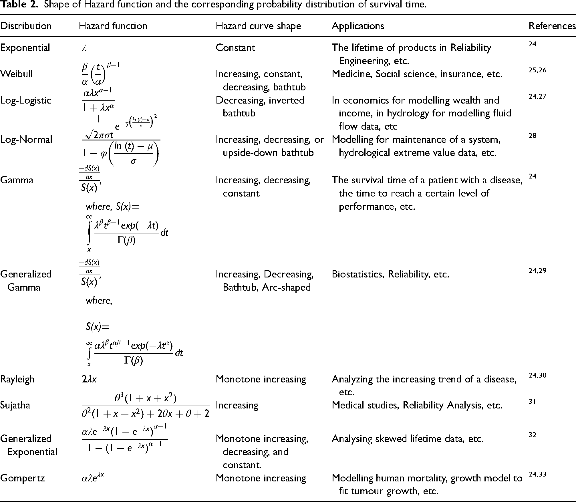
In parametric survival analysis, the survival time is assumed to follow some known probability distribution whose parameters can be estimated from the available data. The general practice of parametric survival analysis is to understand the probability distribution of survival time f(t) from the shape of the hazard curve. For example, a constant hazard rate indicates an exponential distribution, a monotonically increasing or decreasing hazard rate might lead to the Weibull model, a combination of increasing and decreasing hazard with time comes out of the log-normal probability model, and so on.²³ Table 2 provides some common shapes of the hazard function and the corresponding theoretical probability distribution of the survival time.

Table 2.

Shape of Hazard function and the corresponding probability distribution of survival time.

Distribution	Hazard function	Hazard curve shape	Applications	References
Exponential	$λ$	Constant	The lifetime of products in Reliability Engineering, etc.	²⁴
Weibull	$\frac{β}{α} {(\frac{t}{α})}^{β - 1}$	Increasing, constant, decreasing, bathtub	Medicine, Social science, insurance, etc.	^25,26
Log-Logistic	$\frac{α λ x^{α - 1}}{1 + λ x^{α}}$	Decreasing, inverted bathtub	In economics for modelling wealth and income, in hydrology for modelling fluid flow data, etc	^24,27
Log-Normal	$\frac{\frac{1}{\sqrt{2 π} σ t} e^{- \frac{1}{2} {(\frac{l n (t) - μ}{σ})}^{2}}}{1 - φ (\frac{l n (t) - μ}{σ})}$	Increasing, decreasing, or upside-down bathtub	Modelling for maintenance of a system, hydrological extreme value data, etc.	²⁸
Gamma	$\frac{\frac{- d S (x)}{d x}}{S (x)}$ , where, S(x)= $\int_{x}^{\infty} \frac{λ^{β} t^{β - 1} e x p (- λ t)}{Γ (β)} d t$	Increasing, decreasing, constant	The survival time of a patient with a disease, the time to reach a certain level of performance, etc.	²⁴
Generalized Gamma	$\frac{\frac{- d S (x)}{d x}}{S (x)}$ , where, S(x)= $\int_{x}^{\infty} \frac{α λ^{β} t^{α β - 1} e x p (- λ t^{α})}{Γ (β)} d t$	Increasing, Decreasing, Bathtub, Arc-shaped	Biostatistics, Reliability, etc.	^24,29
Rayleigh	$2 λ x$	Monotone increasing	Analyzing the increasing trend of a disease, etc.	^24,30
Sujatha	$\frac{θ^{3} (1 + x + x^{2})}{θ^{2} (1 + x + x^{2}) + 2 θ x + θ + 2}$	Increasing	Medical studies, Reliability Analysis, etc.	³¹
Generalized Exponential	$\frac{α λ e^{- λ x} {(1 - e^{- λ x})}^{α - 1}}{1 - {(1 - e^{- λ x})}^{α - 1}}$	Monotone increasing, decreasing, and constant.	Analysing skewed lifetime data, etc.	³²
Gompertz	$α λ e^{λ x}$	Monotone increasing	Modelling human mortality, growth model to fit tumour growth, etc.	^24,33

However, based on data, when the hazard is computed and plotted empirically, it might not assume any of the forms given in column 3 (Hazard Curve Shape) of Table 2, but rather take some erratic forms. So, when most elite national football teams are expected to score early while playing against the minnows, data paucity is possible, especially in the match's second half. Therefore, erratic forms of hazard function should be reasonably common, and it is customary to fit a smooth curve to enable visualising its underlying shape.²³ Though there are several smoothing methods like spline smoothing, exponential smoothing, lowess smoothing, kernel smoothing, running median, or moving average method, the authors here prefer to use the lowess (locally weighted scatter plot smooth), kernel and spline to tackle the erratic nature of the empirical hazard. One can see Baker and Chambers for the reasons for choosing lowess smoothing over other methods.³⁴

Even after smoothing the hazard curve, if no distinct form is visible, the only way to fit an appropriate probability distribution for modelling survival time is by fitting piecewise distributions. This would make the matter computationally clumsy, but better estimates of the time to the first goal can be accomplished than the one obtained from fitting a single distribution throughout.

From Table 2 and the discussion in the previous paragraphs, the shape of the hazard curve might indicate the corresponding probability distribution of the survival time. However, it might often be confusing as there might be several options, and the process of selecting a particular probability distribution from the shape of the hazard curve might prove to be subjective, so different users may end up reaching different conclusions. Additionally, given the emergence of the possibility of piecewise distribution fitting, the competition amongst distributions may now start for each data segment, emphasising the need to apply objective tools to test the adequacy of fit.

Period of the study

While determining the study period, one cannot go back and start collecting data from a distant past as the team composition and attacking pattern of a national side may change entirely as international matches are not as frequent in football as other team sports like cricket or hockey, so collecting data from the recent past may not provide a considerable number of data points. As the study's objective is to investigate the performance of the selected higher-ranked national football teams against the minnows, further filtering on the international matches played by the selected national football teams should be implemented, leading to an added reduction of data points. The performance of the selected six teams (ranked on June 6, 2023) was analysed over their 250 most recent international matches.

Data source

The data required for this purpose is the time to first goal in matches played by the selected national football teams, specifically, the top six teams, based on their FIFA rankings as of June 2023. For each of these teams, data from their most recent 250 matches were collected. Out of these 250 matches, only those in which the opponent teams were ranked 30 places below (on the day of the match) the high-ranked teams were considered for analysis. Relevant data manually extracted from matches played during the study period are sourced from Soccerway,³⁵ FBref,³⁶ and the InsideFIFA³⁷ website. From the match scorecards, the time to the first goal scored by the respective high-ranked team was taken out for matches against the minnows (i.e., teams ranked at least 30 places below in the FIFA rankings on the day of the match). All calculations and statistical analyses were performed using R software using the FlexSurv and SurvMiner packages and their dependencies.³⁸

Data, analysis and results

As an illustration, the hazard function of Argentina, the team ranked first in the FIFA ranking, is plotted in Figure 1. The plot allows Argentina to score an instantaneous goal while playing against the minnows. The hazard here is the minnows while playing against Argentina.

Figure 1.

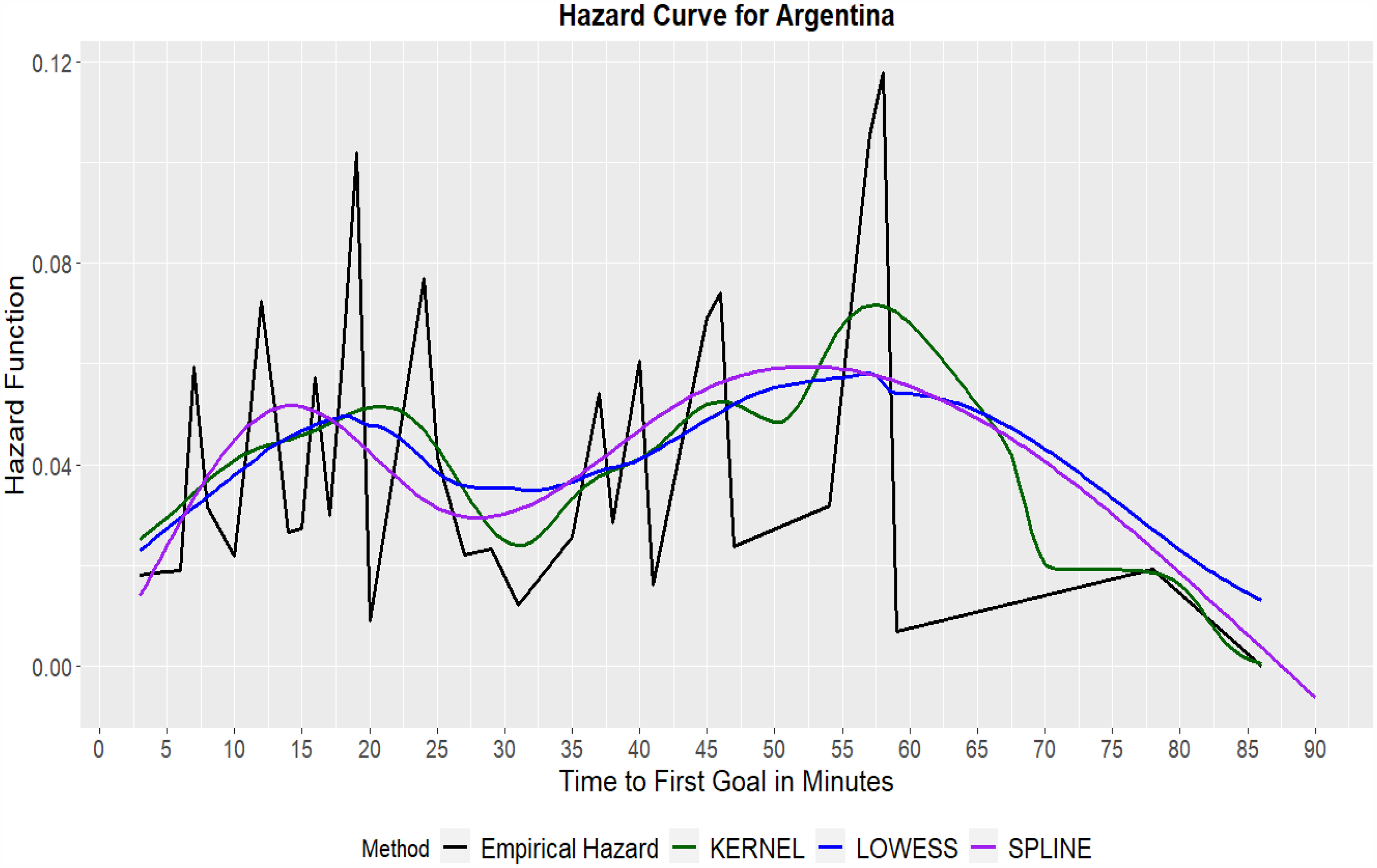
Hazard curve along with the lowess, kernel and spline smoothed techniques for the team Argentina.

Determining the empirical hazard values corresponding to Argentina and plotting the values (c.f. Figure 1) allows the observer to determine the risk of the minnows of conceding a goal. However, the hazard curve thus formed is an unusual zig-zag shape, possibly due to the scarcity of data at various time points. The hazard curve jumps erratically between the different time intervals, as shown by the black line in Figure 1. Cai et al. recommended using a smoothing technique on the hazard function to deal with such situations.³⁹ As discussed in the methodology section, the Lowess smoothing technique is applied and is depicted as a blue line. Additional smoothing techniques, including kernel smoothing (dark green) and spline (purple), are also applied to assess the risk of overfitting. These serve as validation tools, reinforcing the consistency of the observed smoothing patterns.

After plotting the smoothing lines in the figures, the parameter values and their respective AIC and BIC are computed based on the residual variance and the effective number of parameters. Table 3 presents the parameter values along with their respective AIC and BIC scores.

Table 3.

Smoothing parameters and their respective AIC and BIC values.

Model	Parameters			AIC	BIC
Lowess	span = 0.5, effective df = 5.1			−251.7008	−249.7785
Kernel	bandwidth = 8.3, effective df = 3.5			−242.8400	−244.3963
Spline	df = 4	parameters = 5		−145.0365	−135.7044
			Estimate
		(Intercept)	0.013939
		ns (Time, df = spline_df)1	0.003461
		ns (Time, df = spline_df)2	0.056579
		ns (Time, df = spline_df)3	0.072548
		ns (Time, df = spline_df)4	0.037751

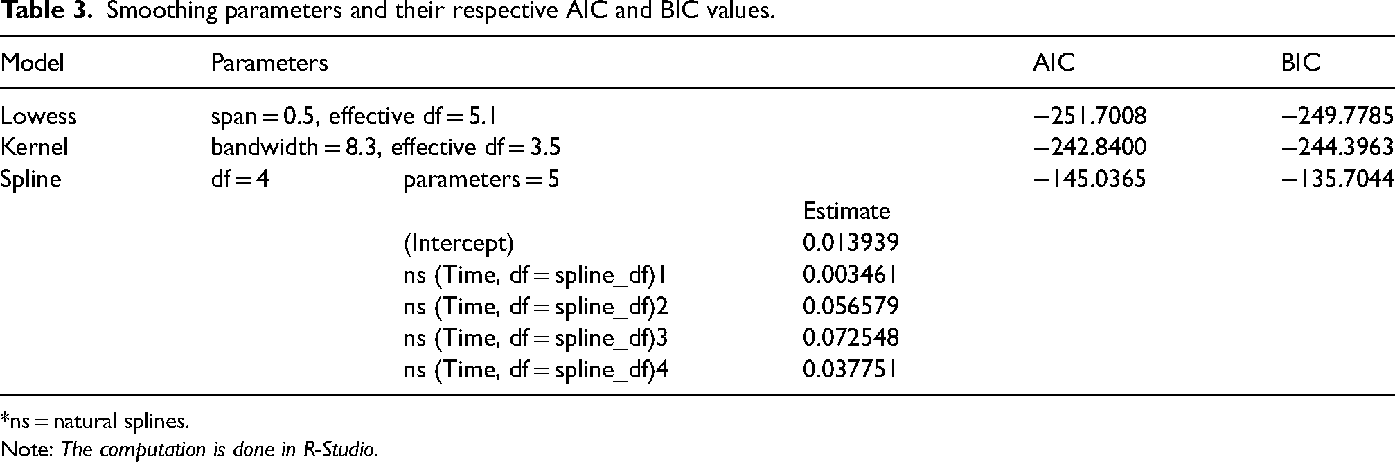
ns = natural splines.

Note: The computation is done in R-Studio.

This table compares three smoothing methods, LOWESS, Kernel, and Spline, used to model a hazard function, evaluated using AIC and BIC. The LOWESS model, with a span of 0.5 and an effective degree of freedom (df) of 5.1, demonstrates the best performance with the lowest AIC (−251.7008) and BIC (−249.7785), indicating an optimal balance between fit and complexity. The Kernel smoothing method, using a bandwidth of 8.3 and an effective df of 3.5, shows slightly higher AIC (−242.8400) and BIC (−244.3963) values, suggesting a less favourable fit compared to LOWESS. The Spline model, with 4 df and 5 parameters, exhibits considerably higher AIC (−145.0365) and BIC (−135.7044) values, indicating a poorer fit or excessive complexity relative to the other methods. Therefore, based on AIC and BIC, LOWESS provides the most suitable smoothing for this hazard function data.

However, in this case, even after smoothing, the hazard curve does not show any monotonic form or any standard form, as discussed in the third column of Table 2. Thus, one may think of looking into the hazard function piecewise to reach known forms of the hazard function. For this purpose, an automated change point detection algorithm, implemented using the ‘pracma’ package in R, was initially employed to identify potential shifts in the hazard rate along the LOWESS smoothed curve. This process yielded many change points, suggesting numerous, potentially major and minor fluctuations. However, among the automatically detected points, two specific time points, 18 and 32 min, were chosen subjectively as they represent two of the major peak change points. To maintain a focus on the most practically significant shifts and to avoid over-complicating the model with excessive piecewise distributions, we opted for a more specific approach, selecting these two key change points. These time points align with critical phases of the game and represent substantial shifts in the hazard rate. Furthermore, the data towards the end of the curve exhibited a sparse distribution, which could lead to unreliable parameter estimation for piecewise distributions. Therefore, we refrained from including change points in this region to ensure robust and meaningful results.

The hazard curve and the identified change points on the LOWESS smoothed line, along with its confidence bands, are presented in Figure 2.

Figure 2.

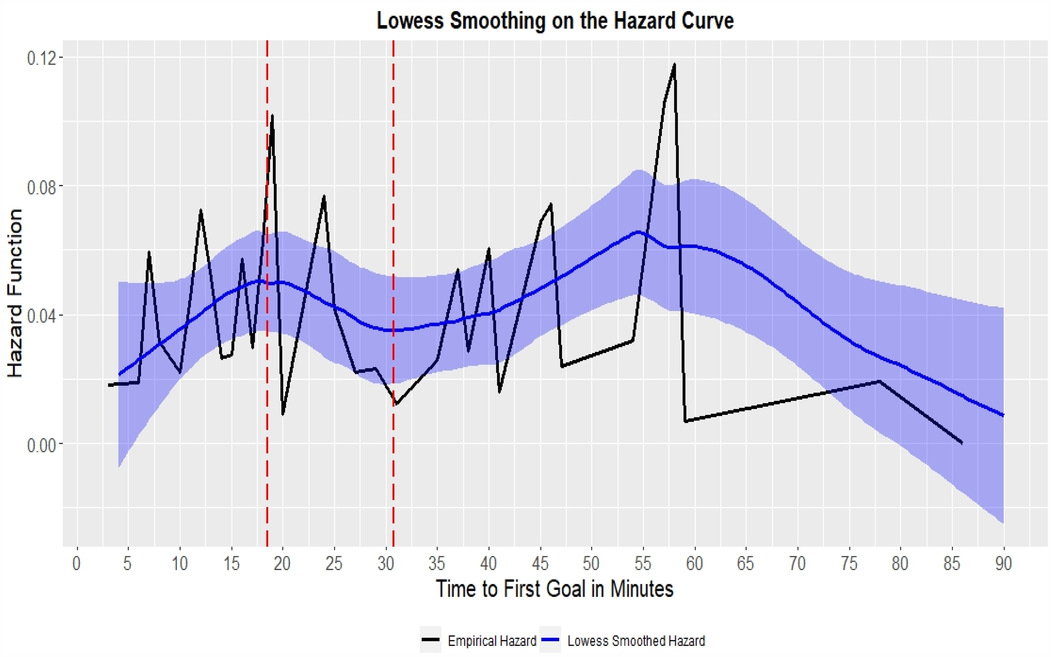
Hazard curve and the LOWESS smoothing along with its confidence bands and the change points.

This leads to identifying a piecewise probability distribution of survival time and thus making three pieces of the hazard curve- increasing hazard (Piece 1: 0 to 18 min), decreasing hazard (Piece 2: 18 to 32 min), and inverted bathtub hazard for above 32 min (Piece 3).

Instantly, different survival distributions mentioned in Table 2 are fitted to the data on the time to the first goal by Argentina in a piecewise manner. The best-fitted survival distribution for each piece is identified and placed in Table 4, along with the modified Kolmogorov-Smirnov goodness–of–fit test appropriate for right-censored survival data, as implemented in the survminer package.

Table 4.

Results of piecewise distribution fitting to survival data for Argentina.

	Best fitted distribution(parameter estimates)	Log-likelihood	K-S statistic	AIC	BIC
Piece 10 to 18 min	Generalized Gamma(μ = 2.89, σ = 0.026, Q = 23.7)	−70.04006	0.095	340.71	354.61
Piece 218 to 32 min	Log-Normal(μ-log = 3.13, σ-log = 0.15)	−29.29715	0.065
Piece 3Above 32 min	Generalized Gamma(μ = 3.68, σ = 0.3, Q = -2.7)	-63.99399	0.081

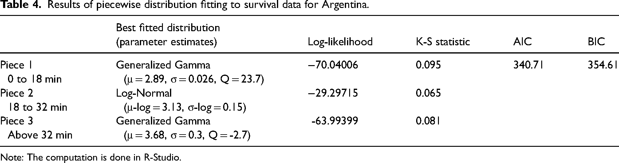
Note: The computation is done in R-Studio.

The researcher assumed that identifying the cut points through a smoothed hazard curve and fitting the piecewise survival time distribution might better fit the parametric survival analysis. To test the claim, the standard survival distributions mentioned in Table 2 are all fitted to the entire Argentina dataset, and it is found that the piecewise fitted distribution has much lower AIC and BIC values compared to any of the other fitted single distributions to the entire data (c.f. Table 1: Appendix 1). Achieving that the piecewise survival distribution with the three pieces fitted with generalised gamma, log-normal and generalised gamma gives the best fit to Argentina's data, the filled survival curve and the empirical survival probability are drawn (Figure 3).

Figure 3.

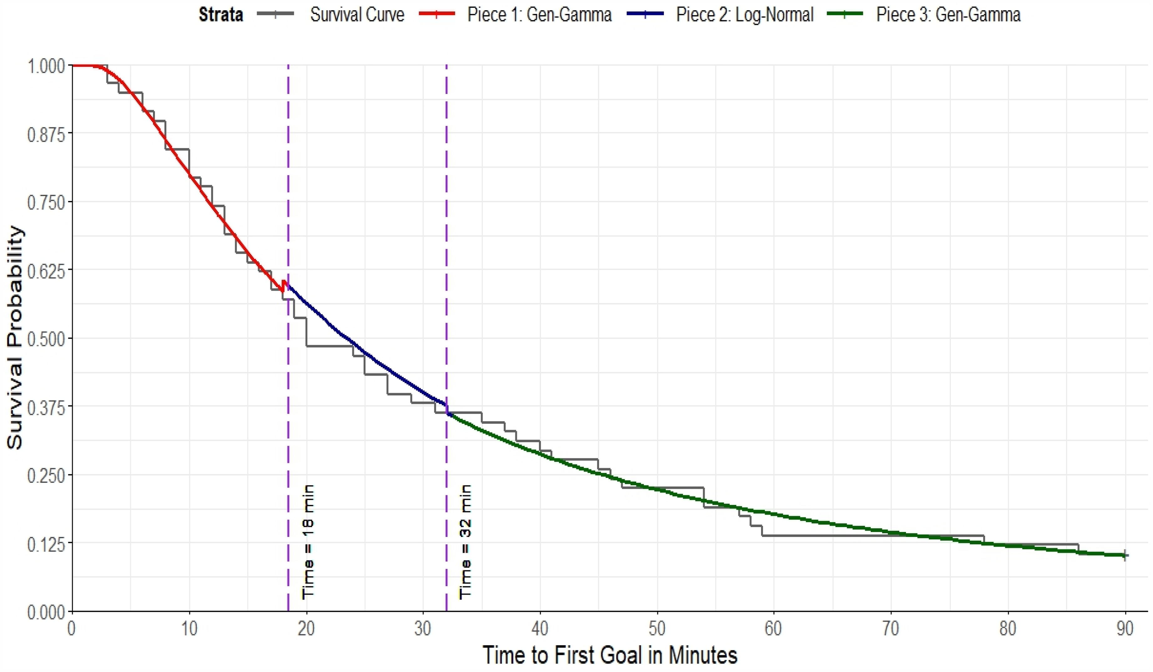
Piecewise fitted survival density to Argentina's data along with the empirical survival probability.

The same exercise is repeated for the other five football teams while encountering the minnows. In all the cases, it was found that piecewise fitting of the best survival time distribution provided a better fit than fitting a single distribution for the entire dataset. The summary of the computations, along with the best-fitted piecewise distributions, is provided in Table 5 below.

Table 5.

Results of piecewise distribution fitting to survival data for Belgium, Brazil, England, France and The Netherlands.

Pieces	Time period(in min)	Distributions	Parameter estimates	K-S statistic	Log-likelihood	AIC	BIC
Belgium
Piece 1	0–54.5	Sujatha	Scale: 0.1374	0.085	-96.33	470.52	492.18
Piece 2	54.5–90	Log-Normal	μ-log: 4.3311	0.025	-35.93
Piece 2	54.5–90	Log-Normal	σ-log: 0.1568	0.025	-35.93
Brazil
Piece 1	0–22	Gompertz	Shape: 0.1380	0.055	-48.55	270.35	284.34
Piece 1	0–22	Gompertz	Rate: 0.0340	0.055	-48.55
Piece 2	22–49	Log-Normal	μ-log: 3.4787	0.039	-41.37
Piece 2	22–49	Log-Normal	σ-log: 0.2345	0.039	-41.37
Piece 3	49–90	Log-Normal	μ-log: 4.4077	0.042	-39.25
Piece 3	49–90	Log-Normal	σ-log: 0.3110	0.042	-39.25
England
Piece 1	0–20	Gamma	Shape: 3.995	0.078	-57.88	331.19	346.98
Piece 1	0–20	Gamma	Rate: 0.418	0.078	-57.88
Piece 2	20–50	Log-Logistic	Shape: 9.05	0.071	-53.23
Piece 2	20–50	Log-Logistic	Scale: 27.91	0.071	-53.23
Piece 3	50–90	Log-Normal	μ-log: 4.4227	0.051	-48.48
Piece 3	50–90	Log-Normal	σ-log: 0.2674	0.051	-48.48
France
Piece 1	0–26	Generalized Gamma	μ: 3.21	0.078	-70.32	336.41	351.87
			σ: 0.032
			Q: 24.7
Piece 2	26–56	Gamma	Shape: 21.756	0.025	-35.37
Piece 2	26–56	Gamma	Rate: 0.552	0.025	-35.37
Piece 3	56–90	Generalized Gamma	μ: 4.04530	0.065	-54.51
			σ: 0.02229
			Q: -21.61789
Netherlands
Piece 1	0 -16.5	Sujatha	Scale: 0.3699	0.012	-34.47	161.31	170.562
Piece 2	16.5–55	Gamma	Shape: 11.985	0.051	-60.64
Piece 2	16.5–55	Gamma	Rate: 0.393	0.051	-60.64
Piece 3	55–90	Log-Normal	μ-log: 4.4604	0.048	-49.49
Piece 3	55–90	Log-Normal	σ-log: 0.2600	0.048	-49.49

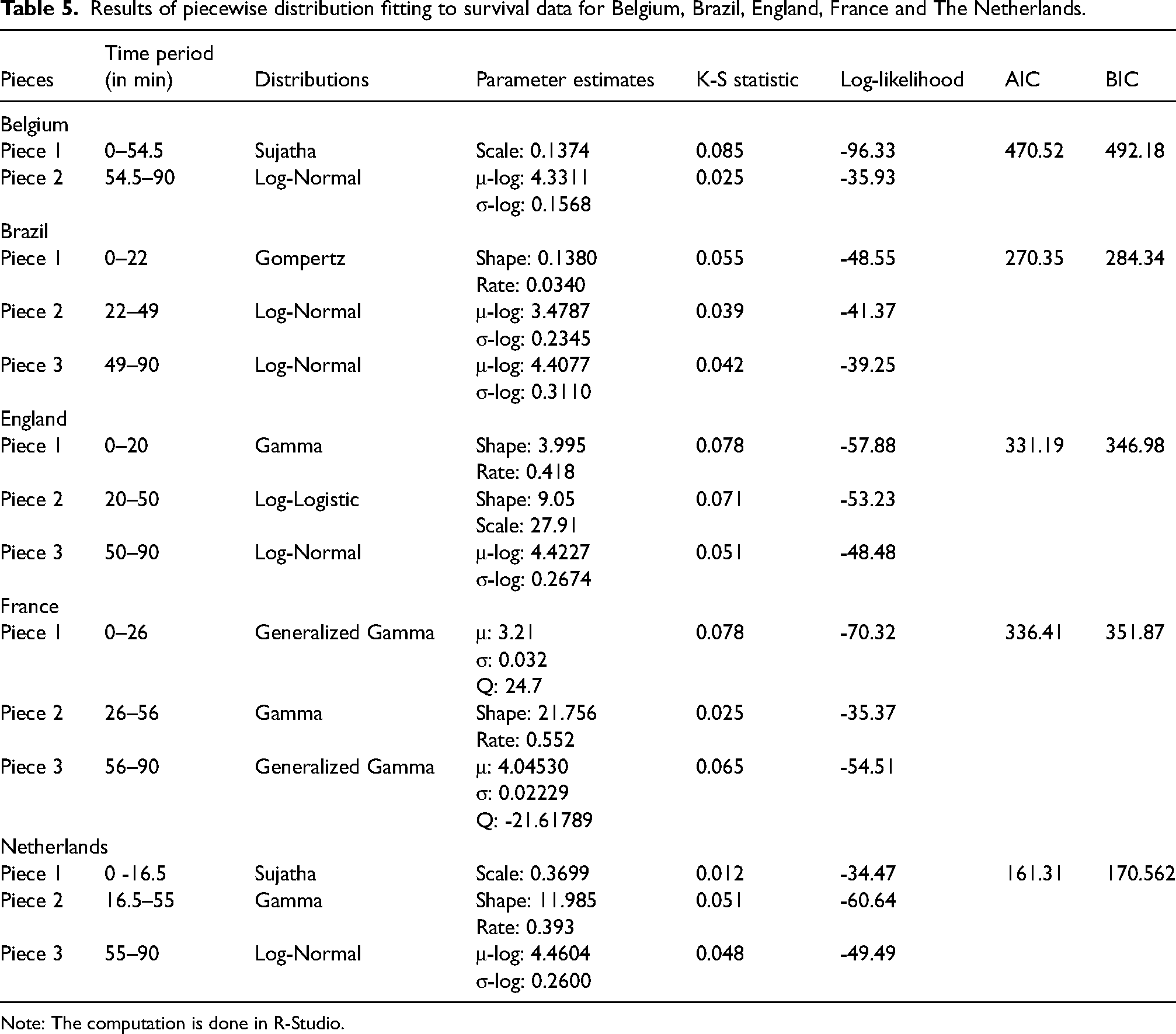
Note: The computation is done in R-Studio.

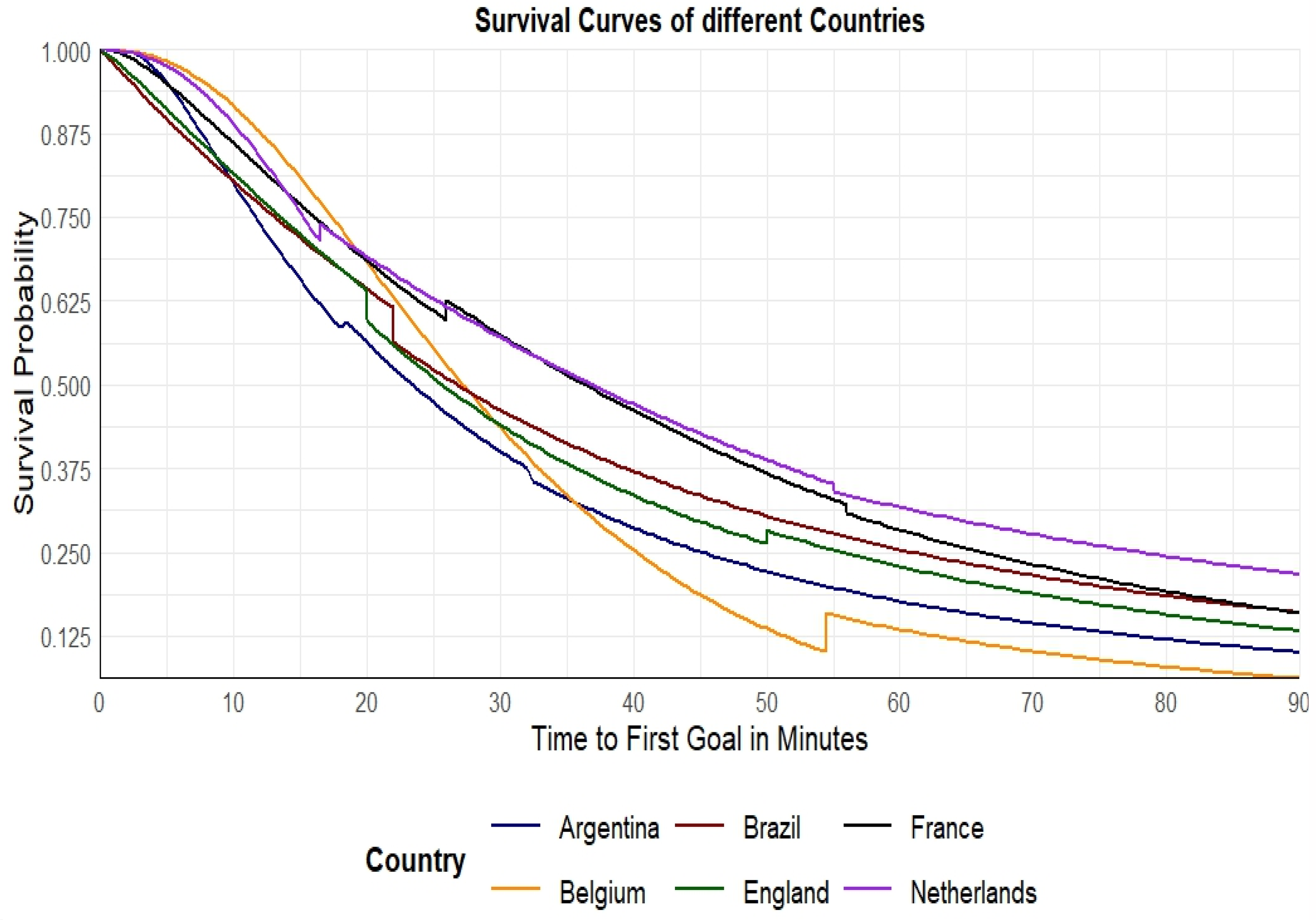
On obtaining the best-fitted distributions of survival time, piecewise fitted in all the cases, the survival curve is now plotted in the same graph so that the performance of the high-ranked sides against the minnows can be compared in Figure 4.

Figure 4.

Fitted survival curves of selected six national football teams while playing the minnows.

However, Figure 4 looks very complicated and interpreting anything meaningful out of the figure in terms of comparing the performance of the teams seems to be a tricky proposition. However, it does not go without debulking any information. The attacking mode of Belgium against the minnows, compared to other teams, can be vivid from the graph. Initially, though the survival chances of opponents (minnows) of Belgium are higher before half-time, the minnows will find it challenging to survive compared to any other strong teams. France and the Netherlands’ patterns are almost similar when encountering the minnows. The highest FIFA-ranked team, Argentina (marked as blue line), comes very strong against the minnows, especially from the 10^th minute till the 35^th minute. During this period, Argentina has been going hard against the minnows compared to the other teams. Even beyond that period, the chance of survival of minnows is not compromised against Argentina as they remain only second to Belgium. Interestingly, Brazil (maroon line), better known for its attacking football, except the first 10 min, takes an average position and seems to be neither too crashing nor too mild while scoring their first goal against the minnows. A similar statement can also be made about England (green). The Netherlands (violet) and France (black) are more compassionate against the minnows than the other selected teams. Especially in the case of the Netherlands, even at the 90^th minute, the survival probability is almost as high as 25 per cent. This means the Netherlands ends up without scoring a goal in 1/4^th of their matches against the minnows. For a better comparison, a pairwise plotting of the fitted survival curves along with the 95 per cent confidence bands is done in Appendix 2.

Discussion and conclusion

The work attempts to apply parametric survival analysis to data related to time to the first goal by six selected national football teams while playing against the minnows, i.e., national football sides that are at least 30 positions below the selected sides as per FIFA ranking. The six highest-ranked national football teams are identified per the FIFA Rankings as of June 2023. Each of the six teams is analysed separately. The data for the purpose, i.e., time to the first goal by the high-ranked teams while playing the minnows within the study period, is collected from the appropriately mentioned platforms. The empirical hazard curve, which is the basis for identifying the appropriate probability distribution for the parametric survival time, does not attain standard forms. The researchers accordingly deal with the hazard function in a piecewise manner. Hence, in the entire range of the match (90 min), different probability density functions are fitted to the survival data, assuring the accuracy of the parametric fit. The piecewise exercise better fits compared to a single survival distribution in the entire dataset for all the higher-ranked national football teams. When comparing the parametric survival probabilities, one can identify how the strong national football sides play against the minnows. It has been seen that while Argentina and Belgium come very strongly against the minnows, scoring goals at an early stage of the match, France and the Netherlands find it difficult to overpower the minnows.

Aligning with our research, a growing body of literature has explored goal timing in football using various statistical and machine-learning approaches. Poisson process models have been widely applied to model goal occurrences, indicating that goal-scoring follows a stochastic process where events happen at a constant rate over time.⁴⁰ Machine learning techniques have also been employed to predict match outcomes and analyse goal-scoring patterns, leveraging complex historical data.⁴¹ Fedrizzi et al. analysed goal distributions during UEFA EURO 2020, illustrating the relevance of probabilistic modelling in understanding goal timing.⁴² Similarly, Le Coz et al. utilised competing risk survival analysis to assess the impact of team formation on goal occurrences, highlighting the role of tactical decisions in shaping match outcomes.⁴³ Furthermore, research has also explored Bayesian and time-dependent models to refine predictions in football analytics.^44,45 This study contributes to this growing field by applying hazard-based modelling to examine how the higher-ranked teams perform against weaker opponents. Unlike traditional Poisson or machine learning models, this approach provides insights into the timing of the first goal when a relatively stronger team tries to break the wall of the minnows. However, as suggested in prior research, integrating additional predictive techniques, such as Bayesian updating or deep learning, could further enhance our understanding of goal-scoring dynamics. Future work may explore these directions to refine goal timing predictions and improve team performance analysis. Additionally, a limitation of this study is the absence of contextual factors such as team composition, match importance, and tactical variations. Integrating detailed match metadata in future research could enhance the analysis and provide a more comprehensive understanding of goal-scoring dynamics.

Though survival analysis or other statistical tools are commonly used in football analytics, the problem addressed here is unique and essential. Taming the minnows by superlative teams in any ball game is always an interesting phenomenon in the arena of sports. While it is generally supposed that a strong team will quickly demolish the minnows, which mostly happens, sometimes such minnows make the road to success very thorny and challenging for the superlative teams. This is not only specific to football but can be applied to other team/individual sports. Thus, an occasional analysis of how superior teams deal with the minnows shall always be in the cards. The paper shows how such a type of analysis can be materialised.

Another remarkable contribution of the paper is the relevance of a piecewise fitting of the survival probability distributions. Though the idea is not novel, an appropriate real-life situation where one feels the need to go for a piecewise fitting is rarely encountered. This work identifies a situation where the piecewise fitting is essential and has proved empirically that this fitting provides better performance than the single distribution fit in six different situations.

So far as the area of further research is concerned, the opportunity to apply this methodology to other sports, with both team and individual events, is open. Encounters between stronger and relatively weaker teams occur every day in all sports. Even in football, one can compare a team's performance against that of a team of equal strength and that of the minnows and note the changeover. For example, one can compare the hazard (or survival) of an opponent in the peer group of Argentina with that of the minnows while playing against Argentina. The deviation of the survival curves should tell the story of Argentina's deviation of aggression while playing the stronger teams and the minnows. When this exercise is carried out with other strong teams, exciting insights can be visible regarding the deviation in the teams’ approaches while facing equally vital teams and the minnows. Another avenue for future research could explore a reverse analytical approach. Specifically, examining the time to first goal conceded by higher-ranked teams, or studying how weaker teams perform offensively against various tiers of opposition, could offer deeper insights into minnows’ adaptability and strategic behaviour. Such an extension would help compare whether defensive or offensive tendencies vary when minnows face teams of similar or dissimilar strength, thereby broadening the understanding of match dynamics from both tactical perspectives.

Footnotes

Data availability

Data have been made available as supplementary files.

Declaration of conflicting interests

The authors declared no potential conflicts of interest with respect to the research, authorship, and/or publication of this article.

Funding

The authors received no financial support for the research, authorship, and/or publication of this article.

Statement of ethics

All data used in this research were obtained from publicly available sources on the Google Search Engine. As this research did not involve human subjects, no ethical approval was required. The researchers adhered to ethical principles by ensuring data integrity and responsible use.

ORCID iDs

Anirban Dutta

Jonali Gogoi

Dibyojyoti Bhattacharjee

Hemanta Saikia

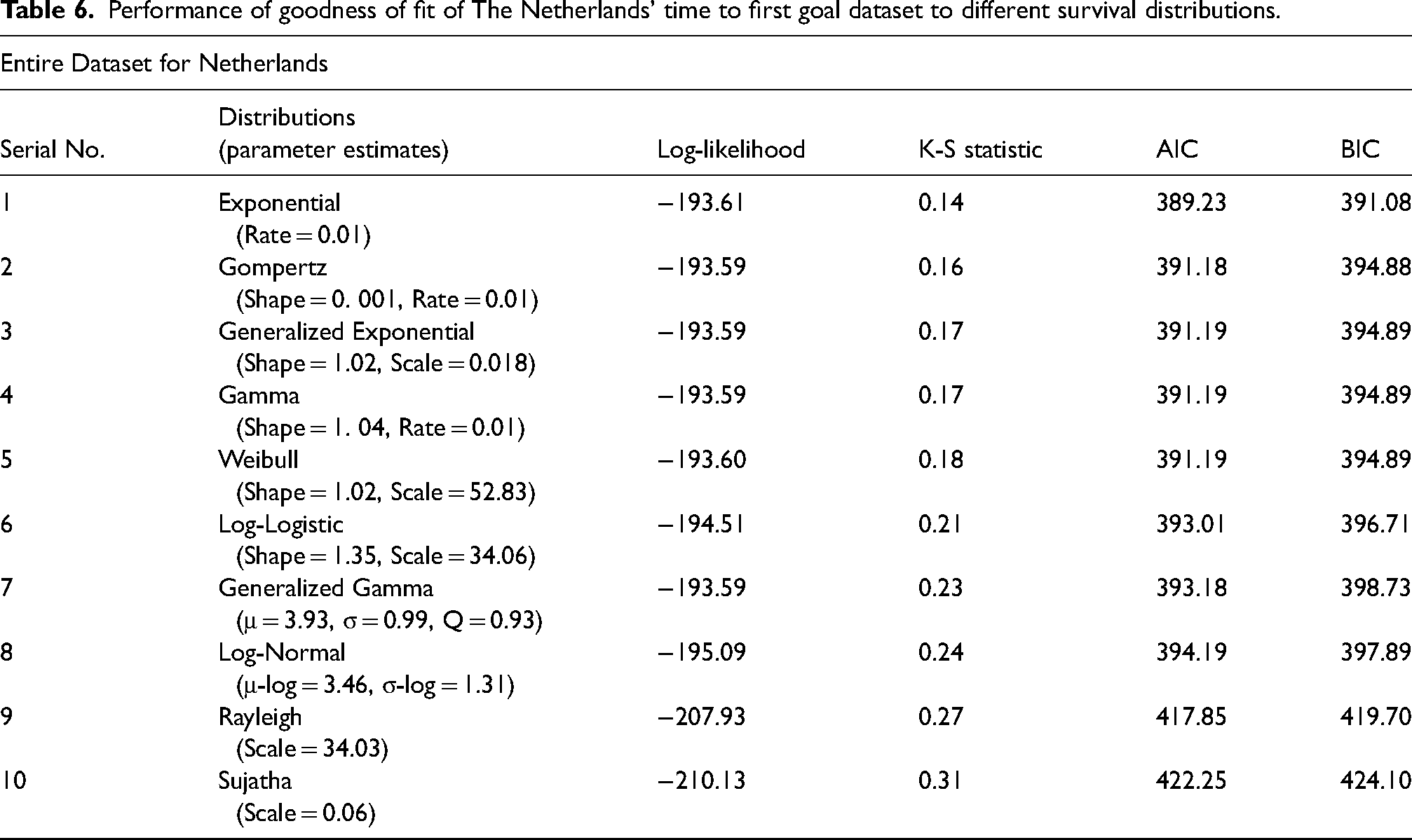
Appendix 1: Important Results related to Distribution Fitting

Table 6.

Performance of goodness of fit of The Netherlands’ time to first goal dataset to different survival distributions.

Entire Dataset for Netherlands
Serial No.	Distributions(parameter estimates)	Log-likelihood	K-S statistic	AIC	BIC
1	Exponential (Rate = 0.01)	−193.61	0.14	389.23	391.08
2	Gompertz (Shape = 0. 001, Rate = 0.01)	−193.59	0.16	391.18	394.88
3	Generalized Exponential (Shape = 1.02, Scale = 0.018)	−193.59	0.17	391.19	394.89
4	Gamma (Shape = 1. 04, Rate = 0.01)	−193.59	0.17	391.19	394.89
5	Weibull (Shape = 1.02, Scale = 52.83)	−193.60	0.18	391.19	394.89
6	Log-Logistic (Shape = 1.35, Scale = 34.06)	−194.51	0.21	393.01	396.71
7	Generalized Gamma (μ = 3.93, σ = 0.99, Q = 0.93)	−193.59	0.23	393.18	398.73
8	Log-Normal (μ-log = 3.46, σ-log = 1.31)	−195.09	0.24	394.19	397.89
9	Rayleigh (Scale = 34.03)	−207.93	0.27	417.85	419.70
10	Sujatha (Scale = 0.06)	−210.13	0.31	422.25	424.10

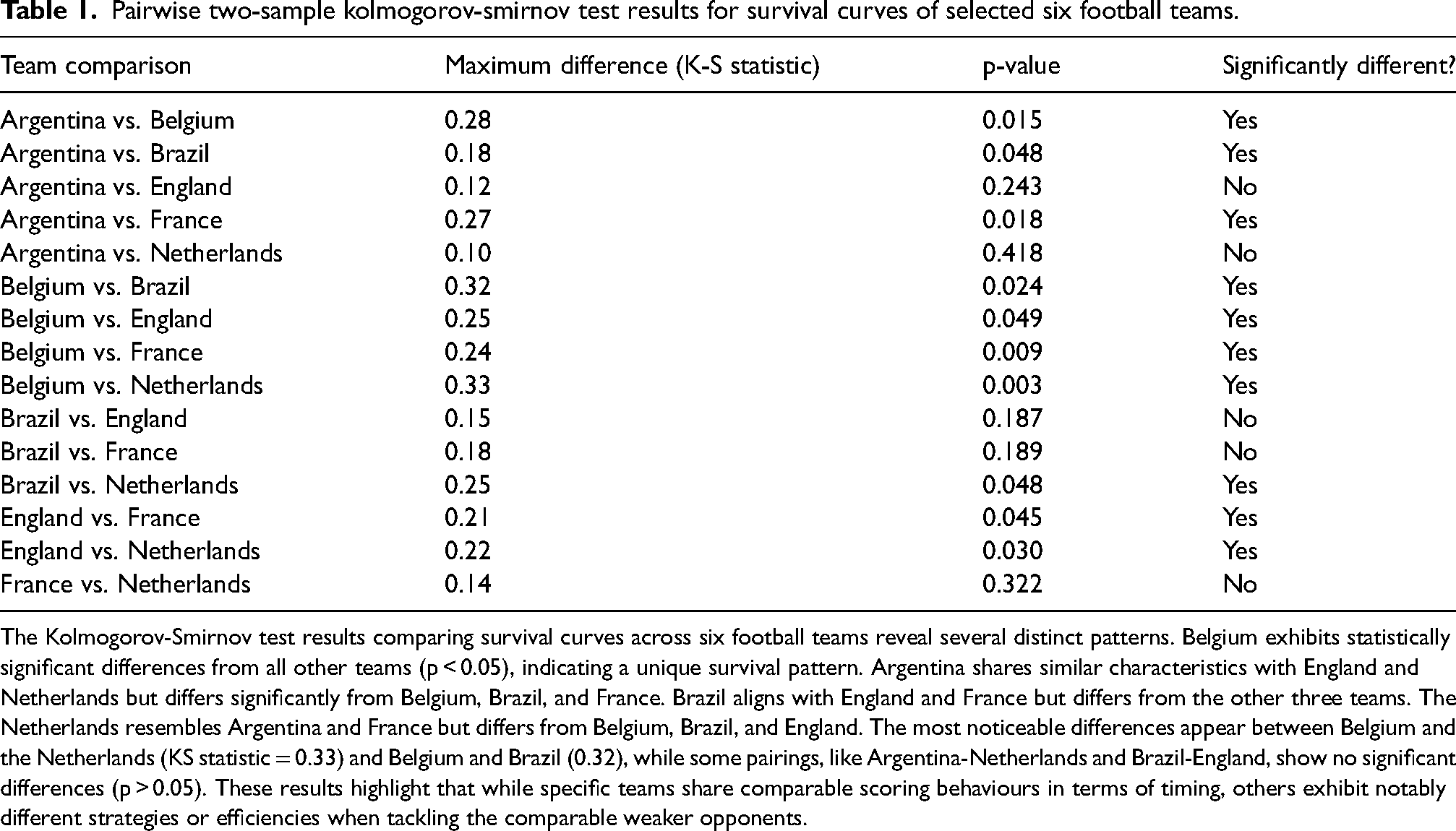
Appendix 2: Individual and Pairwise Fitted Survival Curves of Selected Six National Football Teams (2023) while playing against the minnows

Table 1.

Pairwise two-sample kolmogorov-smirnov test results for survival curves of selected six football teams.

Team comparison	Maximum difference (K-S statistic)	p-value	Significantly different?
Argentina vs. Belgium	0.28	0.015	Yes
Argentina vs. Brazil	0.18	0.048	Yes
Argentina vs. England	0.12	0.243	No
Argentina vs. France	0.27	0.018	Yes
Argentina vs. Netherlands	0.10	0.418	No
Belgium vs. Brazil	0.32	0.024	Yes
Belgium vs. England	0.25	0.049	Yes
Belgium vs. France	0.24	0.009	Yes
Belgium vs. Netherlands	0.33	0.003	Yes
Brazil vs. England	0.15	0.187	No
Brazil vs. France	0.18	0.189	No
Brazil vs. Netherlands	0.25	0.048	Yes
England vs. France	0.21	0.045	Yes
England vs. Netherlands	0.22	0.030	Yes
France vs. Netherlands	0.14	0.322	No

The Kolmogorov-Smirnov test results comparing survival curves across six football teams reveal several distinct patterns. Belgium exhibits statistically significant differences from all other teams (p < 0.05), indicating a unique survival pattern. Argentina shares similar characteristics with England and Netherlands but differs significantly from Belgium, Brazil, and France. Brazil aligns with England and France but differs from the other three teams. The Netherlands resembles Argentina and France but differs from Belgium, Brazil, and England. The most noticeable differences appear between Belgium and the Netherlands (KS statistic = 0.33) and Belgium and Brazil (0.32), while some pairings, like Argentina-Netherlands and Brazil-England, show no significant differences (p > 0.05). These results highlight that while specific teams share comparable scoring behaviours in terms of timing, others exhibit notably different strategies or efficiencies when tackling the comparable weaker opponents.

References

Herberger

Litke

. The impact of big data and sports analytics on professional football: a systematic literature review. In: Digitalization, Digital Transformation and Sustainability in the Global Economy: Risks and Opportunities. Springer Proceedings in Business and Economics. Cham: Springer, 2021. pp.147–171.

Pantzalis

Tjortjis

. Sports analytics for football league table and player performance prediction. In: 2020 11th Int Conf Inf Intell Syst Appl (IISA). IEEE, 2020, pp.1–8.

Yiğit

Samak

Kaya

. Football player value assessment using machine learning techniques. In: Intell Fuzzy Tech Big Data Anal Decis Mak. Proc INFUS 2019 Conf, Istanbul, Turkey, July 23–25, 2019. Cham: Springer, 2020, pp.289–297.

Ötting

. Predicting play calls in the national football league using hidden markov models. IMA J Manag Math 2021; 32: 535–545.

Smith

. 4 best formations for a slow & weaker team. https://soccerprime.com/best-soccer-formations-for-a-slow (2022, accessed 19 February 2025).

FIFA. FIFA World Cup™ archive. https://www.fifa.com/tournaments/mens/worldcup (2022, accessed 19 February 2025).

India Today. Minnows Guam stun Indian football team in World Cup qualifiers. https://www.indiatoday.in/mail-today/story/minnows-guam-indian-football-team-world-cup-qualifiers-stephen-constantine-257935-2015-06-17 (2015, accessed 19 February 2025).

Schumaker

Solieman

Chen

. Sports data mining. New York: Springer, 2010, p. 33–36.

Bonidia

Brancher

Busto

. Data mining in sports: a systematic review. IEEE Lat Am Trans 2018; 16: 232–239.

10.

Martin

. Sports performance measurement and analytics. Upper Saddle River, NJ: FT Press, 2016.

11.

Miller

. Sports analytics and data science: Winning the game with methods and models. Upper Saddle River, NJ: FT Press, 2015.

12.

Drivet

. From the data to the statistical analysis of football: the case of the Italian serie A league. In: Handbook of research on applied data science and artificial intelligence in business and industry. Hershey, PA: IGI Global, 2021, pp.695–710.

13.

Mackenzie

Cushion

. Performance analysis in football: a critical review and implications for future research. J Sports Sci 2013; 31: 639–676.

14.

Hirotsu

Wright

. Using a markov process model of an association football match to determine the optimal timing of substitution and tactical decisions. J Oper Res Soc 2002; 53: 88–96.

15.

Liu

Hohmann

. Applying the markov chain theory to analyze the attacking actions between FC Barcelona and Manchester united in the European champions league finale. Int J Sports Sci Eng 2013; 7: 79–86.

16.

Meyer

Forbes

Clarke

. Statistical analysis of notational AFL data using continuous time markov chains. J Sports Sci Med 2006; 5: 525–532.

17.

Edmans

Garcia

Norli

. Sports sentiment and stock returns. J Finance 2007; 62: 1967–1998.

18.

Memmert

Raabe

. Data analytics in football: Positional data collection, modelling and analysis. Abingdon: Routledge, 2018.

19.

Nevo

Ritov

. Around the goal: examining the effect of the first goal on the second goal in soccer using survival analysis methods. J Quant Anal Sports 2013; 9: 165–177.

20.

Rowson

Campolettano

Duma

, et al. Concussion risk between individual football players: survival analysis of recurrent events and non-events. Ann Biomed Eng 2020; 48: 2626–2636.

21.

Glasson

Bedford

. Modelling the survival of elite Australian rules footballers. In: Proceedings of the Third Annual ASEARC Research Conference, Newcastle, Australia, 2009 Dec 7–8, pp.1–4.

22.

Kleinbaum

Klein

. Survival analysis: A self-learning text. 3rd ed. New York: Springer, 2012.

23.

Clark

Bradburn

Love

, et al. Survival analysis part I: basic concepts and first analyses. Br J Cancer 2003; 89: 232–238.

24.

Taketomi

Yamamoto

Chesneau

, et al. Parametric distributions for survival and reliability analyses: a review and historical sketch. Mathematics 2022; 10: 3907.

25.

Kizılersü

Kreer

Thomas

. Goodness-of-fit testing for left-truncated two-parameter weibull distributions with known truncation point. Aust J Stat 2016; 45: 15–42.

26.

Kızılersü

Kreer

Thomas

. The weibull distribution. Significance 2018; 15: 10–11.

27.

Raqab

Al-Awadhi

Kundu

. Discriminating among weibull, log-normal, and log-logistic distributions. Commun Stat Simul Comput 2018; 47: 1397–1419.

28.

Kurniasari

Widyarini

Warsono , et al. Characteristics of hazard rate functions of log-normal distributions. J Phys Conf Ser 2018; 1338: 012036.

29.

Cox

Matheson

. A comparison of the generalized gamma and exponentiated weibull distributions. Stat Med 2014; 33: 3772–3880.

30.

Elviana

Purwadi

. Parameters estimation of Rayleigh distribution in survival analysis on type II censored data using the Bayesian method. J Phys Conf Ser 2020; 1503: 012004.

31.

Shanker

. Sujatha distribution and its applications. Stat Transit New Ser 2016; 17: 391–410.

32.

Gupta

Kundu

. Generalized exponential distribution: existing results and some recent developments. J Stat Plan Inference 2007; 137: 3537–3547.

33.

Gohary

Alshamrani

Al-Otaibi

. The generalized gompertz distribution. Appl Math Model 2013; 37: 13–24.

34.

Baker

Chambers

. S: An interactive environment for data analysis and graphics. Belmont: Wadsworth, 1984, p.201.

35.

Soccerway. Club teams. https://int.soccerway.com/teams/club-teams/ (accessed 19 February 2025).

36.

FBref. Match results and statistics. https://fbref.com/en/matches/ (2025, accessed 19 February 2025).

37.

INSIDE FIFA. Men’s FIFA World Ranking. https://inside.fifa.com/en/fifa-world-ranking/men (accessed 19 February 2025).

38.

R Core Team. R: A language and environment for statistical computing. Vienna: R Foundation for Statistical Computing, 2024, https://www.R-project.org/ (accessed 19 February 2025).

39.

Cai

Hyndman

Wand

. Mixed model-based hazard estimation. J Comput Graph Stat 2002; 11: 784–798.

40.

Downey

. Think Bayes. 2nd ed. https://allendowney.github.io/ThinkBayes2/chap08.html (2021, accessed 22 February 2025).

41.

Carloni

De Angelis

Sansonetti

, et al. A machine learning approach to football match result prediction. In: HCI International 2021 - posters. Lecture notes in computer science, Vol 12786. Cham: Springer, 2021, pp.473–480.

42.

Fedrizzi

Canal

Micciolo

. UEFA EURO 2020: an exciting match between football and probability. Teach Stat 2022; 44: 119–122.

43.

Le Coz

Iapteff

Rioland

, et al. A competing risk survival analysis of the impacts of team formation on goals in professional football. Front Sports Act Living 2024; 6: 1323930. doi:https://doi.org/10.3389/fspor.2024.1323930.

44.

Groll

Ley

Schauberger

, et al. A hybrid random forest to predict soccer matches in international tournaments. J Quant Anal Sports 2019; 15: 271–287.

45.

Cruz

Ramos

Pinho

. A time-dependent scoring system for soccer leagues. arXiv 2018. doi:https://doi.org/10.48550/arXiv.1803.07981.