
Abstract
This work presents a computational study of atomization in an air-assisted coaxial atomizer utilizing a benchmark configuration, the Sydney Needle Spray, to examine both dense and dilute spray regimes under realistic gas-phase turbulence. A geometric volume-of-fluid method, coupled with large-eddy simulation and adaptive mesh refinement, resolves the interface and surrounding gas flow with high fidelity, and both phases are validated against experiment, providing a robust basis for simulation credibility. With a reasonably good agreement in the overall trend of droplet size distribution relative to the experiment, this study further evaluates the impact of numerical tolerances, showing that the strict settings commonly used in fundamental studies do not necessarily improve accuracy in terms of characteristic droplet size for large-scale spray simulations. Furthermore, the analysis identifies radial velocity fluctuations within the liquid column as an indicator of the onset of liquid-column instability. A thinner boundary layer at the air-pipe exit intensifies interfacial instabilities, leading to enhanced radial velocity fluctuations within the liquid column and improved atomization performance. Finally, the simulations elucidate the atomization sequence: the liquid column first regularizes the core gas flow, interfacial waves then develop and shed liquid sheets, which subsequently fragment into ligaments and droplets, producing intermittent mass-flow-rate signals downstream. Frequency-spectrum analysis of the liquid mass flow rate further reveals subharmonic frequency components corresponding to the merging of successive liquid sheets. The results establish a validated, high-fidelity framework for air-assisted sprays and offer guidance for large-scale spray simulations and an accurate description of the primary breakup processes.
Keywords
Introduction
The demand for high efficiency and reduced emissions for combustion systems continues to increase due to concerns about climate change and air quality. In liquid-fueled combustion systems, such as gas turbines and internal combustion engines, the ability to precisely control atomization plays a critical role in improving combustion efficiency while reducing the formation of pollutants. However, spray atomization is governed by complex, highly coupled physical interactions, making the underlying mechanisms difficult to fully characterize.
Among the various atomization strategies, air-assisted atomizers are widely used in aviation applications 1 because of their capability to produce fine droplets. The Sydney Needle Spray experiment 2 is a well-established benchmark for studying atomization in air-assisted injection systems. It features a coaxial needle-air setup. The recess sets how far upstream or downstream the liquid needle exit is positioned relative to the surrounding air outlet. By adjusting the recess, the setup allows researchers to explore a wide range of spray regimes, from dense, jet-dominated primary breakup to more dilute, droplet-driven dispersion.2–5 Accordingly, with zero recess, the spray forms an intact liquid column, enabling focused investigation of primary atomization. In contrast, a longer recess relocates the primary breakup inside the recessed region, producing a dilute spray at the air exit, which is suitable for studying dispersed-phase dynamics and its effect on combustion. While the Sydney Needle Spray experiments provide valuable insights into jet breakup, physical constraints limit the ability to visualize internal flow structures and breakup dynamics in the dense-spray regime. These limitations hinder direct observation of key mechanisms, making computational fluid dynamics (CFD) a necessary tool for developing a more complete understanding of the atomization process.
There are several computational approaches to model spray atomization. The Lagrangian description of liquid parcels coupled with Eulerian gas-phase flows is most commonly used in engineering simulations. Its main advantage lies in its computational efficiency and relative simplicity, as it models liquid clusters as spheres with aerodynamic forces obtained through empirical correlations. However, it cannot capture interfacial dynamics and resolve non-spherical structures with sufficient fidelity, such as the continuous liquid column formed during primary atomization. Consequently, the Lagrangian method is unsuitable for predicting the initial liquid breakup process and the associated primary atomization mechanisms.
To capture details of the interface dynamics, the volume-of-fluid (VOF) method 6 is an Eulerian approach suited for dense-spray atomization problems, where a volume-fraction field is used to track each phase by solving a volume-fraction transport equation. The method is effective in describing the primary breakup process in dense sprays, where liquid structures behave collectively rather than as individual droplets. An interface capturing method using the VOF method is typically implemented using either algebraic or geometric approaches.
The algebraic VOF method solves for the volume fraction in each computational cell using an algebraic approximation of the volume-fraction transport equation. Because the interface is not reconstructed explicitly and is instead represented by cell-averaged volume fractions, it tends to smear the interface over multiple cells unless strong compressive schemes are employed. Despite their known limitations, the algebraic VOF methods remain the most commonly used approach in favor of their computational efficiency. These methods are further classified into compressive schemes and tangent of hyperbola for interface capturing 7 schemes according to the formulation of the volume-fraction flux. 8
Examples of compressive VOF schemes include compressive interface capturing scheme for arbitrary meshes, 9 switching technique for advection and capturing of surfaces, 10 high-resolution artificial compressive formulation, 11 and the high-resolution interface capturing (HRIC). 12 In the HRIC, the cell-face volume fraction is obtained from a piecewise HRIC scheme defined within the admissible normalized variable diagram region, which limits interface smearing by adopting a downwind scheme while preserving boundedness through blending toward the upwind scheme. This method was applied to the Sydney Needle Spray 13 using a fine grid resolution and demonstrated promising accuracy. However, the study employed highly non-uniform grid spacing in the axial direction, which may introduce numerical inaccuracies during interface evolution, leading to the unnatural droplet morphologies observed along the axial direction.
More recently, a hybrid turbulence filtering with artificial compression (TF-AC) model14,15 has been proposed. This method selectively applies an artificial compression term to sharpen the interface between continuous liquid and gas, while activating standard turbulence filtering only in regions containing discrete liquid structures such as ligaments and droplets. However, the model relies on a grid-dependent parameter. 16 When used in simulations of the Sydney Needle Spray, it was found that both spray and gas-phase dynamics change significantly with grid resolution for a given model parameter. 17
To mitigate issues associated with the grid-dependent parameter, the explicit volume diffusion (EVD) model 18 was developed. This model computes the surface tension force using a subgrid-scale (SGS) term that incorporates a physical length scale, rendering the formulation independent of grid resolution. The EVD model was also tested for the Sydney Needle Spray configuration and showed improved agreement with experimental data compared with the TF-AC model. 17 However, the EVD model still requires a model constant for the evaluation of surface tension forces, which makes it less general than methods based on first principles.
In contrast to the algebraic VOF methods, the geometric VOF methods explicitly reconstruct the interface geometry within each computational cell containing the interface. Although this approach is more computationally demanding, it represents the sharp liquid–gas interface without numerical interface diffusion and provides improved mass conservation, 19 making it well-suited for spray modeling that requires accurate prediction of ligament formation and breakup. The most common approach for reconstructing the interface using geometric approximations is the piecewise linear interface calculation (PLIC) technique, 20 in which the interface is represented as a plane within a computational cell. As a result, the geometric VOF methods eliminate the need for artificial compression terms while maintaining a sharp interface. The geometric VOF method with PLIC reconstruction has also been applied to the Sydney Needle Spray configuration. 21 However, the predicted radial variation of droplet axial velocities shows limited agreement with experimental data. This indicates that further investigations are required when applying the geometric VOF methods to practical spray simulations, such as the Sydney Needle Spray.
The present study employs a high-fidelity geometric VOF method to model atomization in the Sydney Needle Spray, eliminating interface diffusion and achieving accuracy beyond what is attainable with the algebraic VOF approaches used in previous studies.13,17 To ensure simulation fidelity, a joint validation of both spray dynamics and gas-phase flow characteristics has been carried out which is an aspect that has not been considered in previous studies.13,17,21 This joint validation is essential because gas-phase turbulence and aerodynamic interactions are among the dominant mechanisms driving atomization. 22 While strict solver tolerances are commonly adopted in fundamental studies, they are often impractical for the large-scale, long-duration simulations required to obtain statistically converged spray characteristics. Nevertheless, the influence of such numerical settings on large-scale atomization predictions remains insufficiently explored. Accordingly, the present work investigates the impact of solver tolerances on large-scale spray simulations in terms of both accuracy and computational efficiency, with the aim of establishing practical guidance and best-practice recommendations for the accurate numerical modeling of air-atomized sprays.
Building on the robust numerical modeling framework, physical mechanisms governing air-assisted atomization are further examined. In particular, the gas–spray interaction is examined to elucidate how the boundary-layer thickness developing within the coaxial air pipe controls the intact liquid-column length,23,24 together with the identification of an indicator of liquid-column instability. In addition, the spectral characteristics of the downstream liquid mass flow rate are analyzed to elucidate the dominant instability modes associated with coherent spray structures. By combining enhanced numerical modeling with new physical insights into air-assisted atomization, this work advances the understanding of spray dynamics and contributes toward the design of more efficient combustion systems aimed at mitigating global warming.
Methods
VOF method
In the present modeling, the VOF approach
6
tracks the liquid–gas interface by recording the volume fraction of the liquid phase, denoted as
The interface is reconstructed from the volume fraction using the
Large-eddy simulation
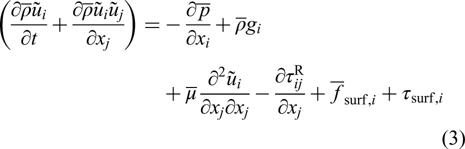
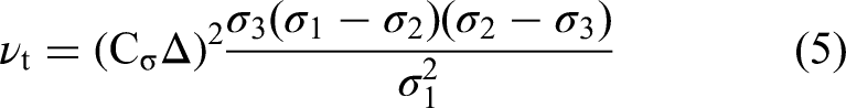
There is no universally accepted set of governing equations for LES of multiphase flows. 28 Generally, there are three primary approaches to LES modeling for multiphase flows: the low-pass filtered version, the Favre-filtered version, and the volume-averaged version. In this study, we adopt the Favre-filtered version, which has been validated under specific conditions. 29 The governing equations involve four unclosed terms: the residual in the divergence of the Favre-filtered velocities, the convective SGS term, the diffusive SGS term, and the SGS surface tension term. Accordingly, based on an order-of-magnitude analysis by Ketterl et al., 29 the residual in the divergence of the Favre-filtered velocities is negligible. Likewise, the diffusive SGS term has a much smaller order of magnitude and can be considered negligible in most cases, as evidenced by several a-priori analyses.30,31
By neglecting these less significant unclosed terms, the governing equations, shown in equations (2) and (3), describe the fundamental conservation laws. Equation (4) models the grid-resolved surface tension force,

The term
The term
The composition
Computational setup for simulation: Air-assisted atomizer
Geometry, parametric conditions, and boundary conditions
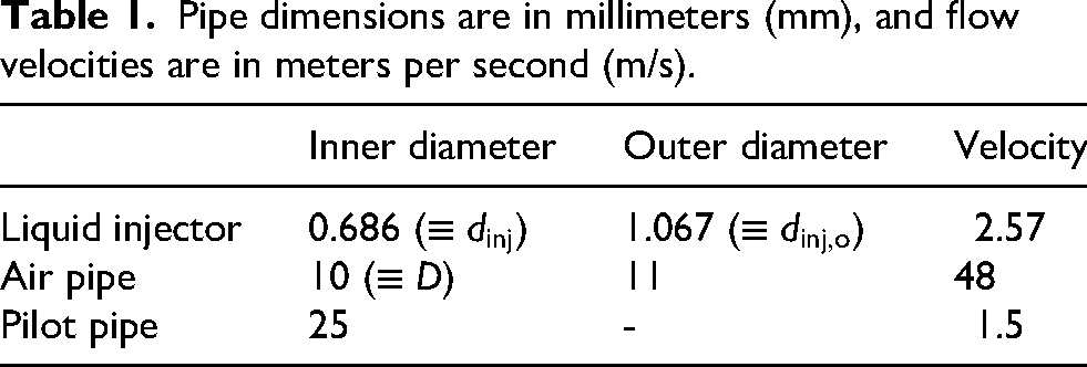
In the Sydney Needle Spray configuration,2–5 the recess is defined as the distance between the exits of the liquid and air pipes. Three recess lengths of 0, 25, and 80 mm are examined in this study. While simulations were performed for all configurations, the comparison presented here focuses on the recess lengths for which corresponding experimental data are available. Figure 1 illustrates the 0 mm recess configuration, and the other configurations share the same geometric components, differing only in the recess length. The geometry dimensions are summarized in Table 1, where
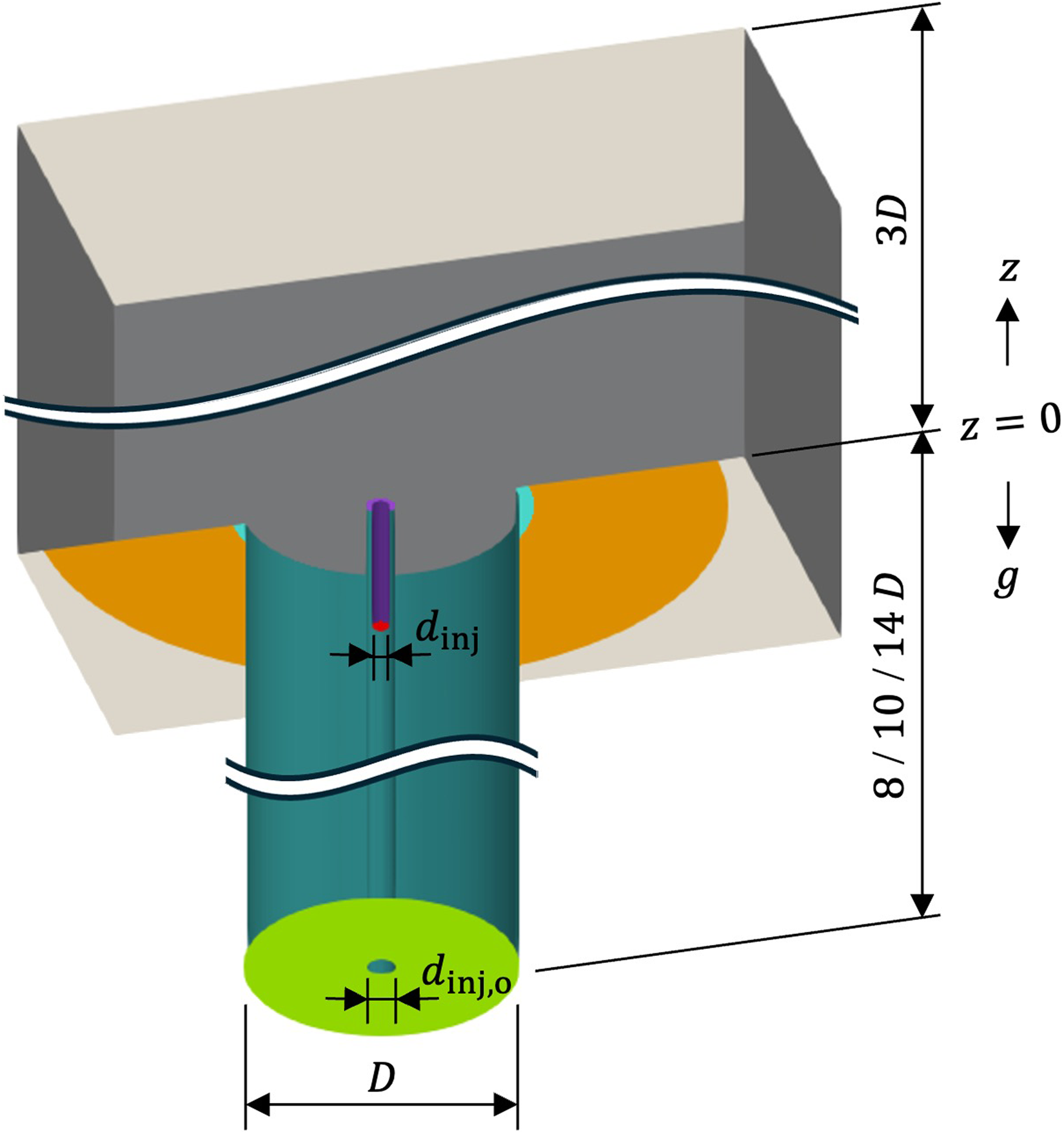
Sectional view of the recess 0 mm configuration, with components represented as follows: liquid inlet (red), liquid injector (purple), air inlet (green), air pipe (blue), pilot inlet (orange), and an open space (gray).
Pipe dimensions are in millimeters (mm), and flow velocities are in meters per second (m/s).
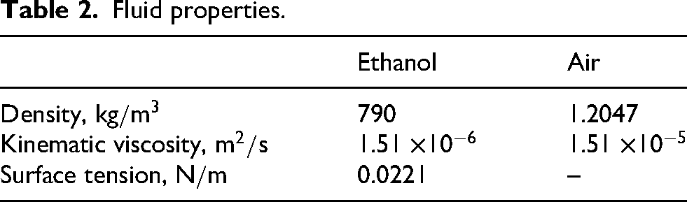
Ethanol is injected from the central liquid injector at an average velocity of 2.57 m/s (represented in red and purple in Figure 1) into an open space (gray). It is injected with a fully developed parabolic velocity profile corresponding to a liquid-phase Reynolds number (
The fluid properties are given in Table 2. Both sets of parameters are chosen to match the experimental conditions of Singh et al. 3 to ensure accurate simulation.
Fluid properties.
Liquid-wall boundary conditions may influence spray formation in the injector. In this study, the volume-fraction boundary condition on the injector wall is prescribed as a zero-gradient condition,
Solution algorithm, numerical schemes, and tolerances
The solver is derived from
The choice of numerical schemes plays a critical role in maintaining accurate liquid-volume conservation in the geometric VOF methods. Liu et al. 34 demonstrated that using a first-order implicit time-integration scheme together with an upwind discretization for the momentum convection term is essential for preserving consistency between the phase-specific volumetric flux and the mass flux in the geometric VOF formulations. Therefore, a first-order implicit scheme is adopted in the present work, while the momentum convection term is discretized using the limited-linear divergence scheme, identified as the next most accurate option in their study.
To further minimize liquid-volume conservation errors in the geometric VOF simulations, careful adjustment of the
Spatial and temporal resolutions
The computational grid consists of four mesh levels, with cell sizes ranging from 31.2 to 250 µm. AMR is applied to resolve interfacial dynamics, enforcing a minimum cell size of
The adaptive refinement and unrefinement procedures in the AMR framework closely track interface motion to avoid redundant cells and optimize computational efficiency. For example, in the 25 mm recess configuration, the total cell count increases from
The time step in this simulation is dynamically adjustable with a maximum velocity Courant number of 0.3 and a maximum volume-fraction Courant number of 0.2 to ensure both accuracy and numerical stability while maintaining computational efficiency.
Near-wall treatment for gas dynamics
To capture the effects of the boundary layer that develops along the coaxial air-pipe wall without incurring prohibitive computational cost, a wall function (
Following the guidelines of Kawai and Larsson
35
and Larsson et al.,
36
the first off-wall grid point in a wall-modeled LES should lie between 0.02 and 0.1 of the local boundary layer thickness,
For wall-modeled LES, the choice of numerical scheme for the convective term has a strong influence on accuracy. 37 Moreover, when wall functions are used together with SGS models that incorporate physical wall damping, such as the sigma model, turbulent structures within the first off-wall grid cell are neither resolved by the grid nor represented by the SGS model. 38 These inaccuracies are accepted as necessary compromises in the present study to ensure robust liquid-volume conservation, which in this work requires the use of a more diffusive convective scheme, as discussed in the Numerical-schemes section.
Validation
A joint examination of both spray dynamics and the surrounding turbulent gas flow is essential because gas-phase turbulence and aerodynamic interactions are among the dominant mechanisms driving atomization. 22 Accordingly, in this study, turbulence development is first investigated by varying the length of the coaxial air pipe in the computational domain and analyzing its influence on spray behavior. Subsequently, for the selected air-pipe length, the gas-phase velocity field is validated in the far field for the longer-recess configuration, which generates a dilute spray regime.
Figure 3 presents an instantaneous snapshot of the spray evolution for the Sydney Needle Spray. The figure highlights the dimensionless spatial locations and the recirculation region downstream of the liquid injector, which are referenced in the following analysis.
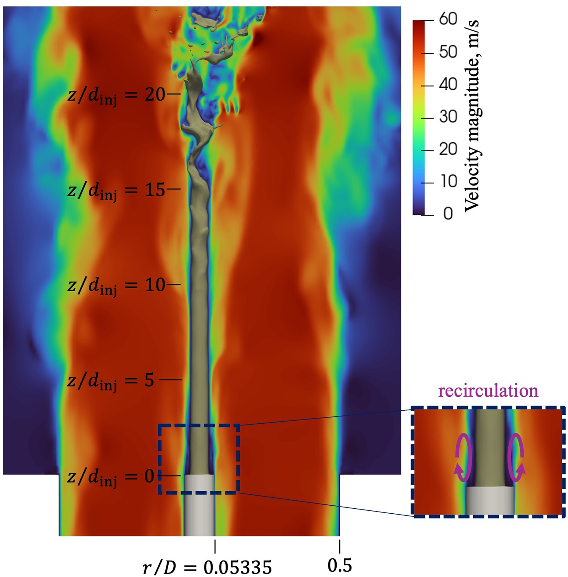
The spray pattern of the Sydney Needle Spray: liquid spray (dark yellow), liquid injector (gray), and gas velocity magnitude (colormap) with an air-pipe length of 10
Spray dynamics
Spray dynamics are strongly influenced by the surrounding gas flow. Therefore, a careful treatment of the inlet gas-flow boundary condition and the axial extent of the coaxial air pipe is essential. Although the turbulence intensity is reported for the wind tunnel supplying air to the injector,
3
its downstream decay and spatial distribution remain unclear. Therefore, prescribing a turbulence intensity directly at the air-inlet boundary could introduce bias. Instead, a uniform inlet velocity is imposed, and turbulence is allowed to develop along the length of the coaxial air pipe. To assess how coaxial air-pipe length influences turbulence development and the resulting spray dynamics, three lengths are evaluated: 8
The liquid presence probability along the injector centerline (Figure 4) is used as a validation metric for the spray model. These data are available only for the 0 mm recess because optical access to the liquid core is limited for the recessed configuration. Experimentally, liquid presence probability is determined by computing the liquid volume fraction within 90 µm sampling cubes along the centerline, sampled at 5000 Hz.
4
The measurement carries an uncertainty of about 20% for spray measurements.
39
For error estimation, symmetric bounds of
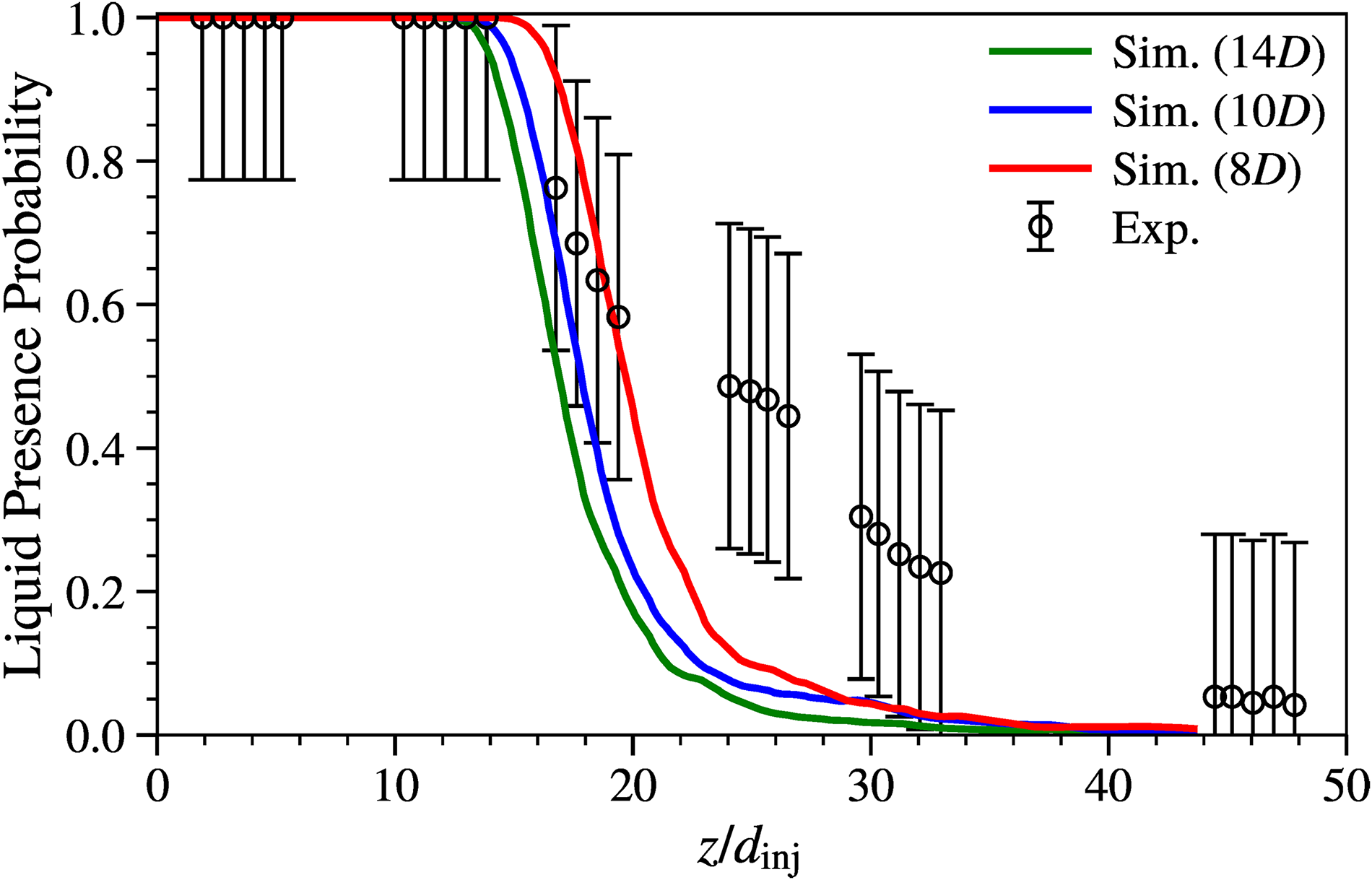
Comparison of the liquid presence probability along the injector centerline for the recess 0 mm configuration: Three solid lines represent simulation results averaged over two liquid injection flow-through times with various lengths of the air pipe. Black markers signify experimental measurements, 4 with error bars indicating the 95% confidence interval.
In the simulation, the experimental sampling method is replicated. Computational cells along the centerline are mapped onto densely distributed 90 µm cubes, with each cell assigned to only one cube to avoid duplication. For each cube, the normalized volume fraction is computed as the ratio of liquid volume in the assigned cells to their total volume. Sampling is performed at every time step and weighted by the time step to produce a time-averaged result. The total sampling duration is
Revisiting the spray dynamics predictions in Figure 4, the 8
The persistent overprediction of the decay rate of liquid-presence probability is likely related to an inaccurate surface tension force, which fails to resist lateral deflection from the centerline. This deficiency may arise from inaccuracies in curvature estimation using the CSF model. 27 Because curvature is a second-derivative quantity, even small numerical errors in the underlying scalar field can be greatly amplified. The CSF model computes curvature directly from the sharply varying volume-fraction field, making it prone to numerical noise and limited in accuracy even when grid resolution is increased. 41 Consequently, merely refining the mesh near the interface is insufficient to resolve the deficiency in the surface tension force and the corresponding error in the decay rate. As future work, higher-order curvature evaluation methods, such as the RDF-based approach, 26 will be explored to improve model fidelity.
The spray patterns for the three cases are shown in Figure 5, together with arrows indicating the liquid-column length, as determined from the liquid presence probability along the centerline shown in Figure 4. The differences observed among the cases with varying air-pipe lengths provide an opportunity to analyze the underlying physical mechanisms responsible for the distinct spray behaviors. These mechanisms are examined in detail in the section on gas–spray interactions.
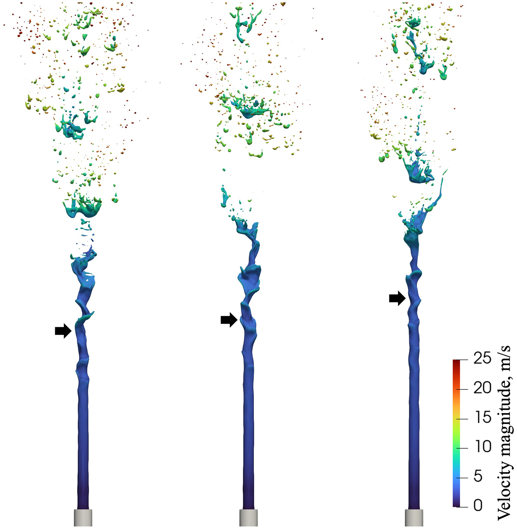
Spray patterns generated by different air-pipe lengths (left: 14
Gas flows
To further validate gas-phase predictions for the 10
Axial acetone-droplet velocities obtained under the 80 mm recess geometry are used for comparison since direct gas-velocity measurements are unavailable in the experiments. This most-dilute configuration is therefore selected for gas-velocity validation using pure-gas simulations. The experiment samples along a line, whereas the simulation samples over a plane and reports azimuthal averages over approximately eight flow-through times. Using this protocol, gas velocities are compared against droplet velocities.
At 3 mm downstream of the air-pipe exit (Figure 6(a) and (c)), noticeable discrepancies occur near the centerline (
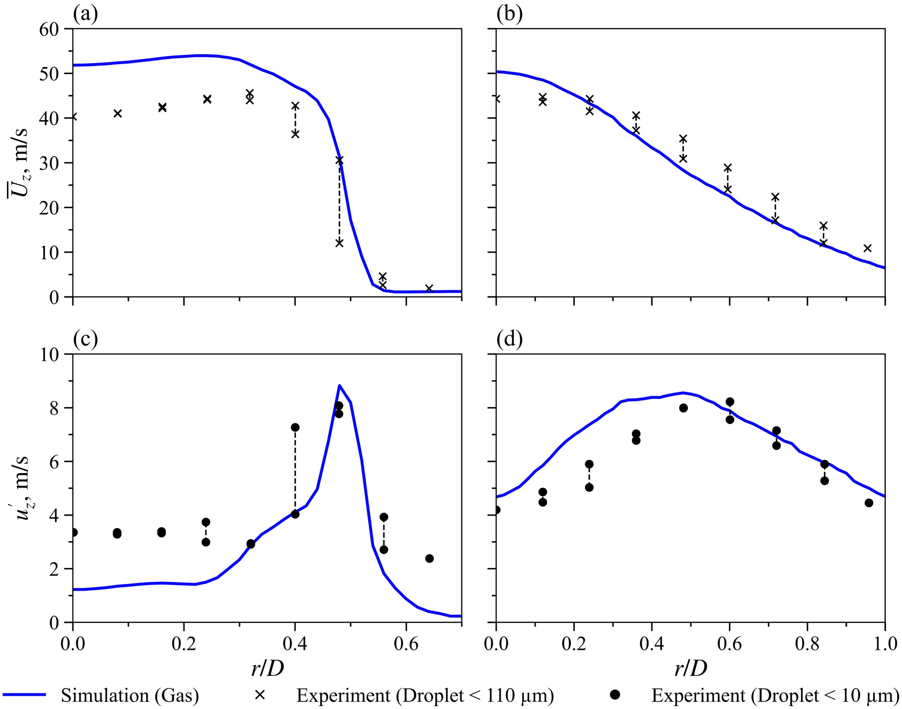
Gas flow validation at 3 mm (a, c) and 50 mm (b, d) downstream of the air-pipe exit for the recess 80 mm configuration, showing mean axial velocity (a, b) and root-mean-square (RMS) axial velocity (c, d). Axial gas velocity from the pure-gas simulation (blue lines), sampled on a plane over approximately eight flow-through times, is compared with acetone droplet axial velocities from the experiment: 2 Crosses denote droplets smaller than 110 µm, dots signify droplets smaller than 10 µm, and dashed lines connect two values measured at the same radial position due to line sampling in the experiment.
Overall, the simulations jointly reproduce key features of both spray dynamics (the liquid-column divergence point from the centerline) and the gas flow (mean and RMS velocities). This demonstrates consistent accuracy across phases, an essential requirement for reliable spray modeling in air-assisted atomizers.
Evaluation of solver tolerances
In most fundamental studies, the tolerances are typically very strict (e.g. Appendix A). However, for practical large-scale spray simulations that require long durations to obtain statistically converged results, such strict settings become prohibitively expensive. To evaluate how tolerance levels affect both accuracy and computational cost in large-scale spray simulations, coarser tolerance configurations (10
A single droplet
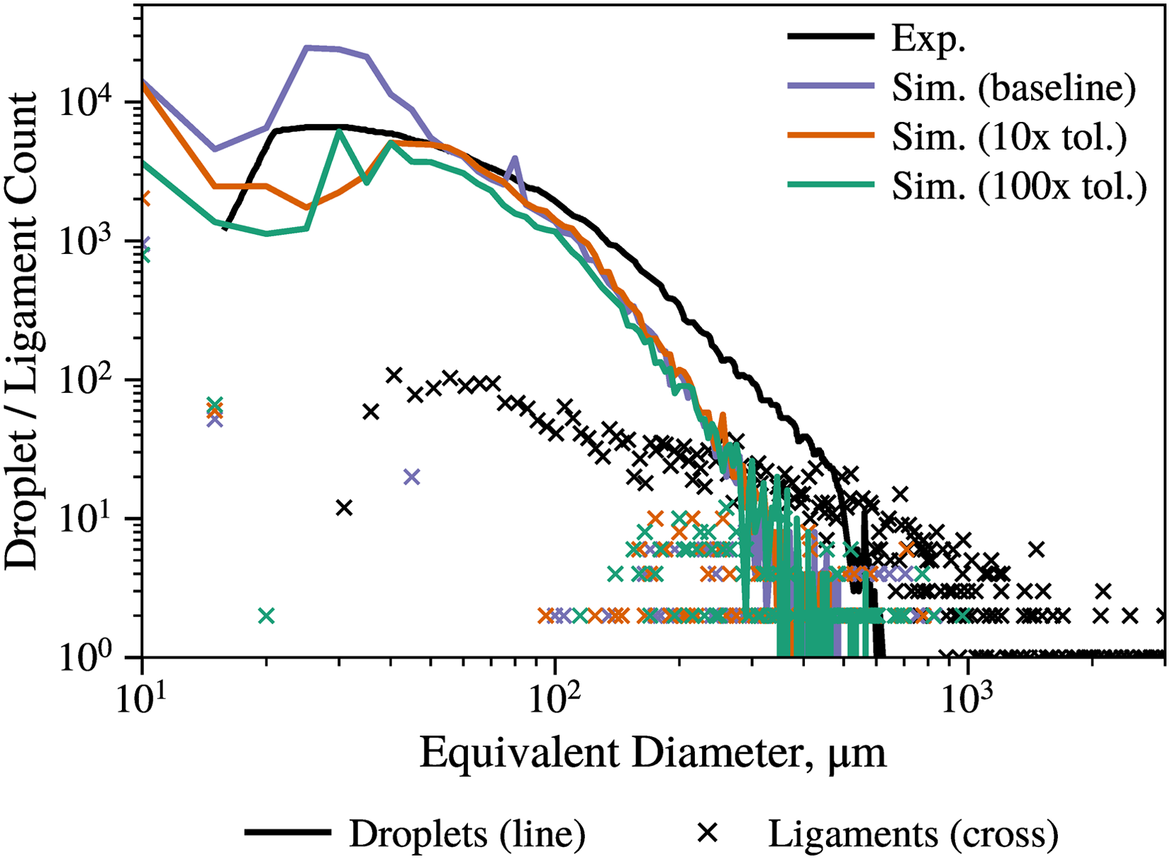
A three-dimensional stagnant droplet with a diameter of 1 mm (blue in Figure 7) is first initialized. Breakup is then induced by prescribing a uniform inlet velocity of 48 m/s at the left boundary, generating numerous secondary droplets by 2 ms (red in Figure 7). AMR is employed in this test case, with a base-grid size of 250 µm and a finest-grid size of 31.2 µm, matching those used in the spray simulations.
Fidelity test of liquid-volume conservation: An initially stagnant blue droplet breaks up into red fragments.
Figure 8 presents the temporal evolution of the absolute value of the relative error in liquid-volume conservation. This error is defined as the deviation of the instantaneous liquid volume,
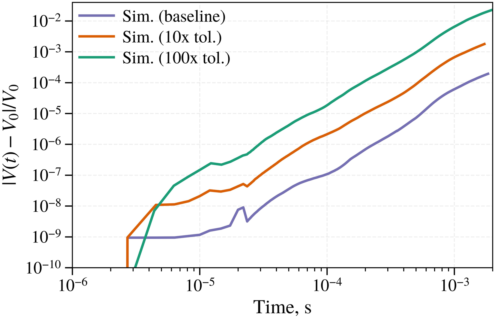
Time evolution of the liquid-volume-conservation error for a stagnant droplet broken up by gas flow.
The lifetime of droplets within the computational domain in our spray simulations is typically <1–2 ms. Within this timescale, the 100
More generally, each spray simulation should be benchmarked under similar conditions using a simple configuration to assess whether the liquid-volume-conservation error associated with coarser tolerances remains acceptable over the droplet lifetime in the computational domain. This result from the simplified test case provides a solid foundation for evaluating volume-conservation behavior prior to analyzing the full spray configurations.
Spray
Solver tolerances can affect both accuracy and efficiency. This investigation seeks to determine whether the strict tolerances commonly adopted in fundamental studies are beneficial in practical spray simulations by addressing two central questions: (i) how numerical tolerances influence the accuracy of practical spray simulations, as quantified by droplet and ligament size distributions (Figure 9) and characteristic metrics (Table 3); and (ii) how the computational cost varies with tolerance level, as measured by the number of pressure-equation iterations (Figure 10) and the normalized wall-clock time (Figure 11).
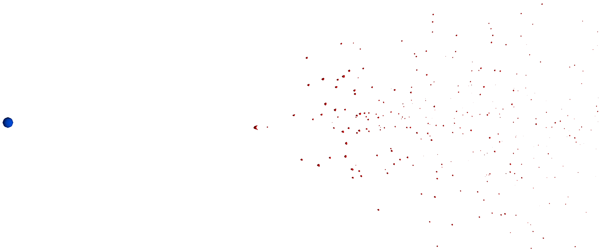
Droplet and ligament size distributions at the air-pipe exit for the 25 mm recess configuration compared with the experiment: 4 Simulation results are sampled over approximately two liquid injection flow-through times and scaled by the rounded ratio of droplet counts between the experiment and the baseline simulation, evaluated at a diameter equal to two grid spacings.
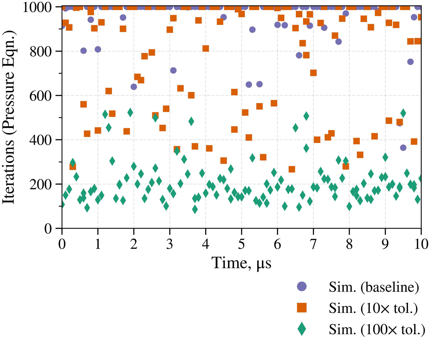
Iteration counts for solving the pressure equation within the first PISO loop of the first PIMPLE loop at each time step for different tolerance sets, plotted against relative time during the early fully atomized stage, when the number of computational grids is similar across the different simulations.
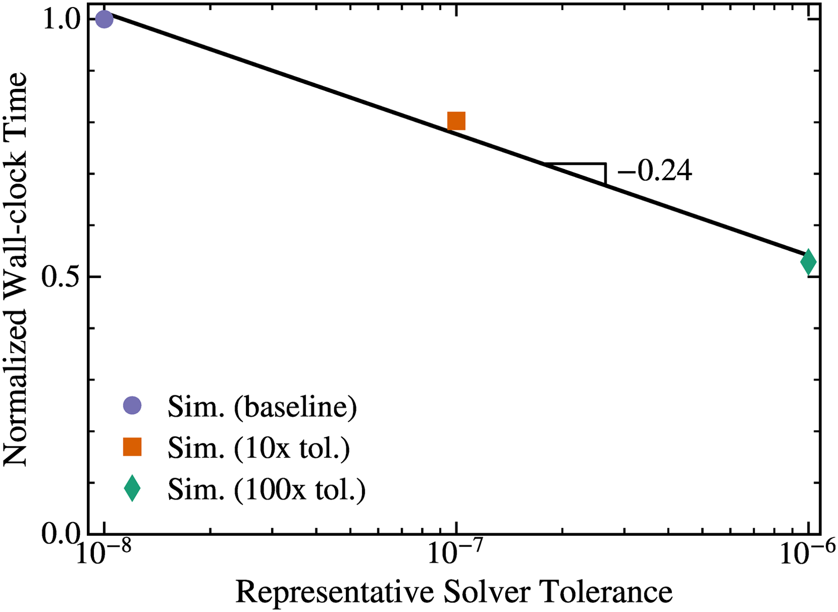
Wall-clock time normalized by the baseline case during the early fully atomized stage, shown as a function of representative solver tolerance for different tolerance sets.
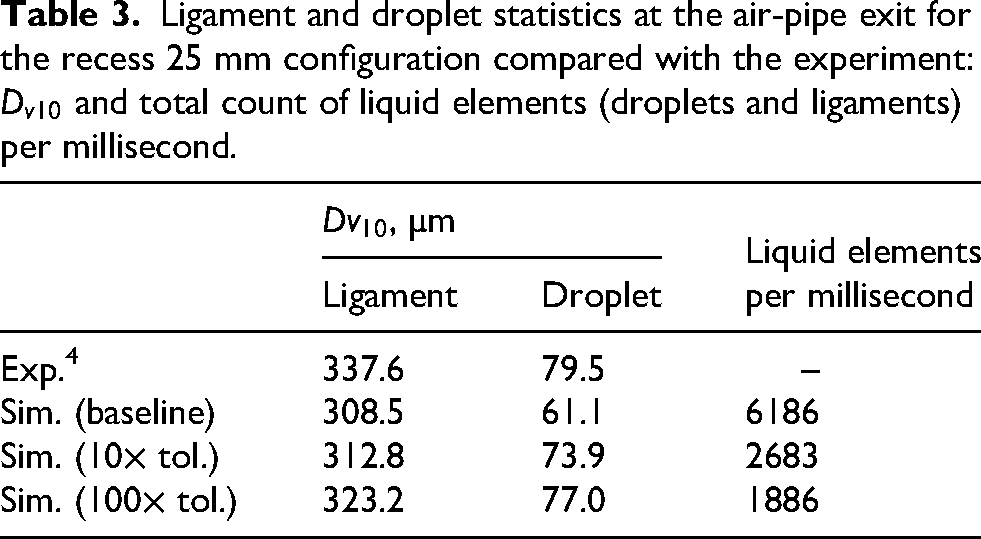
Ligament and droplet statistics at the air-pipe exit for the recess 25 mm configuration compared with the experiment:
The simulations in this section are conducted for the 25 mm recess configuration, employing the 10
Figure 9 presents ligament and droplet size distributions, for which the classification of ligaments and droplets differs between the experiment and the simulations. The experiment uses aspect ratio and size relative to the injector, including a separate category for large objects. 4 In contrast, the present simulation uses sphericity for classification, where droplets have sphericity > 0.4 and ligaments < 0.4, following Lee et al. 42 In their study, clusters were categorized into three types: fibers (aspect ratio > 3 and sphericity < 0.4), ligaments (aspect ratio < 3 and sphericity < 0.4), and spheroids (aspect ratio < 3 and sphericity > 0.4). Because aspect ratio data are not available in the present simulation, classification is simplified using only sphericity, and the fiber category is omitted to enable a consistent two-class comparison with the experimental data. As the large-object category represents only 1% of the total clusters in the experiment, it is not included as a validation target for the current simulation.
The droplet size distribution reproduced by the simulation cases successfully captures the experimental trend, including the location of the peak droplet size. However, two key discrepancies are observed. First, the predicted number of small droplets is overestimated. Second, for sizes larger than the peak, the predicted droplet size distribution exhibits a steeper decay compared to the experimental results. These discrepancies are likely attributable to limitations in interface curvature estimation and insufficient spatial resolution near the interface. As discussed in the preceding chapter, the CSF model used for curvature estimation suffers from limited accuracy, which can weaken the computed surface tension force and thereby promote premature breakup, potentially explaining both discrepancies. Furthermore, when liquid structures approach the grid scale, the inherent limitations of the geometric VOF method induce artificial breakup, producing excessive small droplets and contributing further to the first discrepancy. This issue may potentially be addressed by transforming small liquid objects represented in the volume-fraction field into Lagrangian droplets, which is identified as a direction for future work.
The ligament size distribution shows noticeable discrepancies between the experiment and the simulation. In the experiment, the distribution exhibits a broader spread, encompassing both larger and smaller structures, with a peak near the minimum ligament size followed by a rapid decrease in ligament count toward smaller sizes. In contrast, the simulation predicts a more concentrated range between 90 and 900 µm, along with a non-smooth distribution for ligaments smaller than 50 µm. These discrepancies arise from limited grid resolution, which introduces significant inaccuracies in interfacial area estimation, used for sphericity calculation and subsequent ligament classification, when the liquid clusters approach the size of approximately two grid spacings (about 62 µm) and the interface is reconstructed using a planar approximation within each grid cell.
Despite these discrepancies, the simulations successfully capture the overall trends of the droplet size distributions, demonstrating good qualitative agreement with the experimental observations. However, this qualitative comparison does not reveal clear differences among the various tolerance sets. Therefore, a more detailed quantitative assessment based on the statistical properties of both ligaments and droplets is provided in Table 3.
The characteristic diameters of ligaments and droplets,
According to Table 3, both droplet and ligament
The number of liquid elements passing through the sampling plane per millisecond, summarized in Table 3, provides important clues. These metrics show that looser tolerances lead to less aggressive breakup, resulting in larger
To draw more definitive conclusions regarding the accuracy benefits of varying tolerance levels in such applications, future work should focus on reducing uncertainties arising from differing definitions used to classify ligaments and droplets between experiments and simulations, as well as on mitigating spurious currents. Addressing these fundamental numerical uncertainties will enable a more robust and conclusive assessment of how solver tolerances influence size distributions and spray characteristics in large-scale atomization.
To evaluate the computational cost, the number of iterations required to converge the pressure equation is examined, as it typically dominates the overall cost of the PIMPLE algorithm. As illustrated in Figure 10, the baseline case exhibits iteration counts that frequently reach the maximum limit of 1000, indicating repeated failure to achieve the prescribed residual tolerance. The case with tolerances coarsened by a factor of 10 exhibits similar behavior, with frequent occurrences of the maximum iteration count and a substantial number of iterations clustered around 400. In contrast, the case with tolerances relaxed by a factor of 100 shows a pronounced reduction in iteration counts, with most values falling between 100 and 300. Figure 11 further presents the normalized wall-clock time for the simulations over a longer time interval. Relaxing the tolerances by two orders of magnitude reduces the wall-clock time by
When the computational-cost trends shown in Figures 10 and 11 are considered alongside the accuracy results in Figure 9 and Table 3, it becomes evident that the strict tolerances commonly employed in fundamental studies offer limited accuracy benefits while incurring approximately double the computational cost for practical large-scale spray simulations under the current numerical formulation and simulation configuration. To further substantiate this conclusion more generally, future work should focus on improving the accuracy of the numerical methodology and post-processing procedures, as well as on testing a broader range of simulation cases.
Interactions between gas flows and spray
Given that gas-phase turbulence and aerodynamic interactions constitute the dominant mechanisms driving the atomization process, 22 a thorough assessment of the surrounding gas flow and its coupling with spray dynamics is essential.
Boundary layer in the air pipe
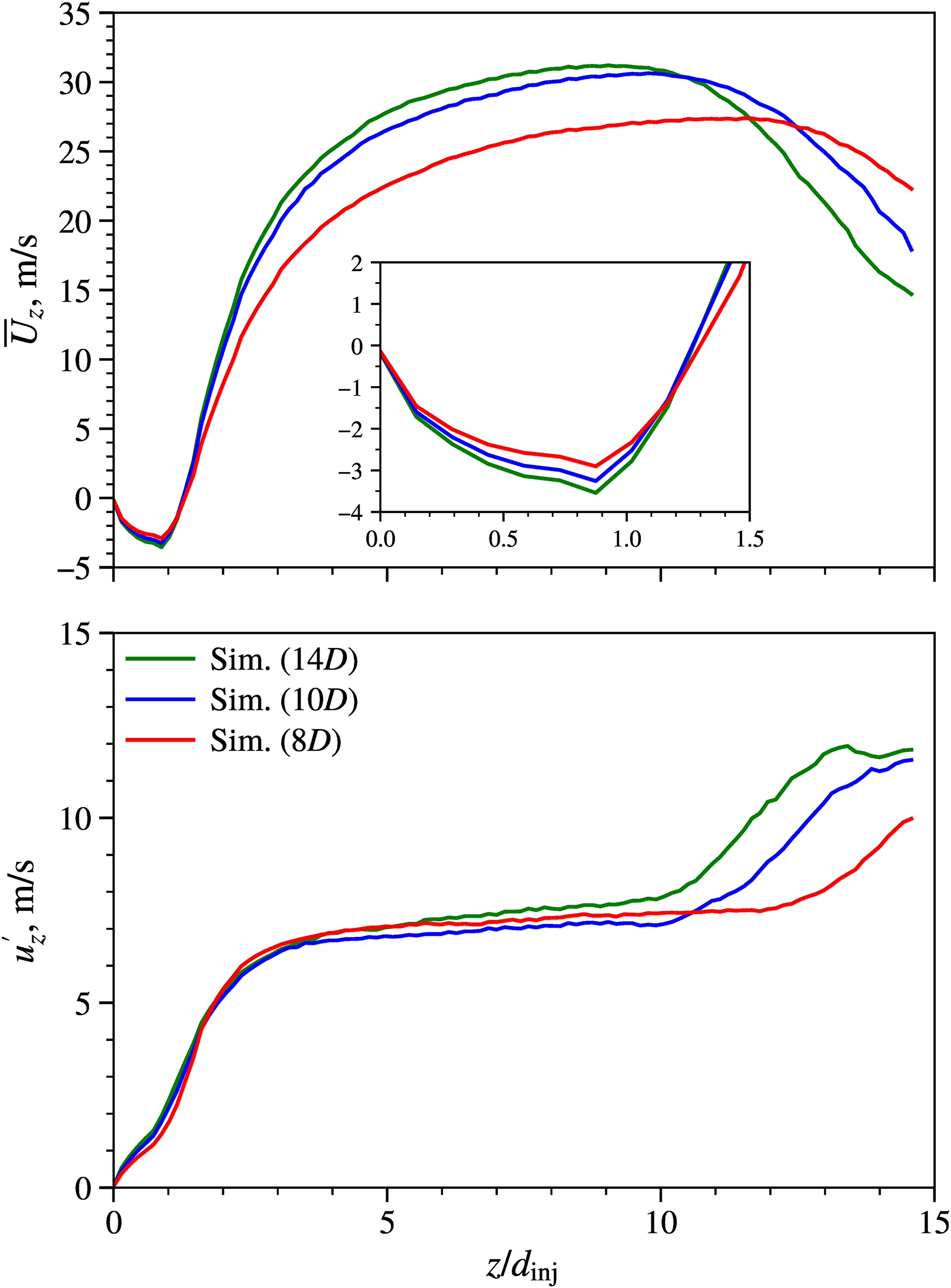
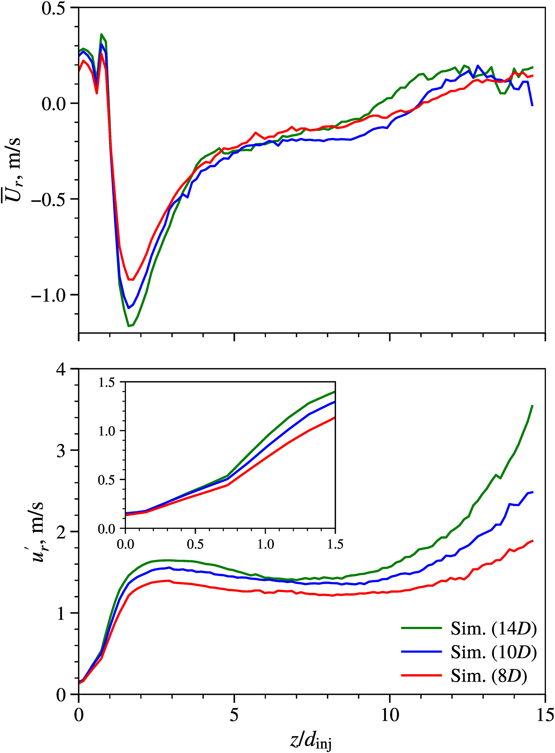
The different gas-flow profiles produced by the three air-pipe lengths (8
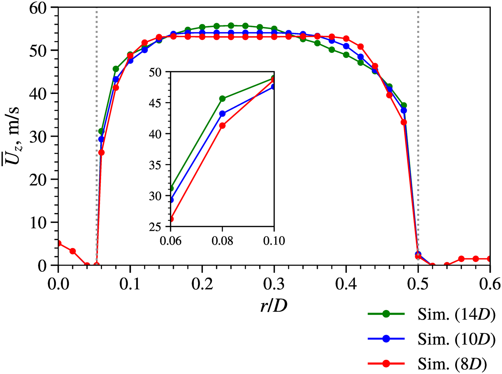
Mean axial velocity (
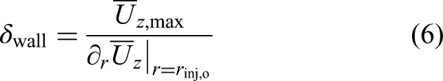
The boundary layer thickness on the outer wall of the liquid injector at the air-pipe exit, denoted as
Radial velocity fluctuation in the liquid column
Figure 13 presents the radial velocity fluctuations along the injector centerline. The 14
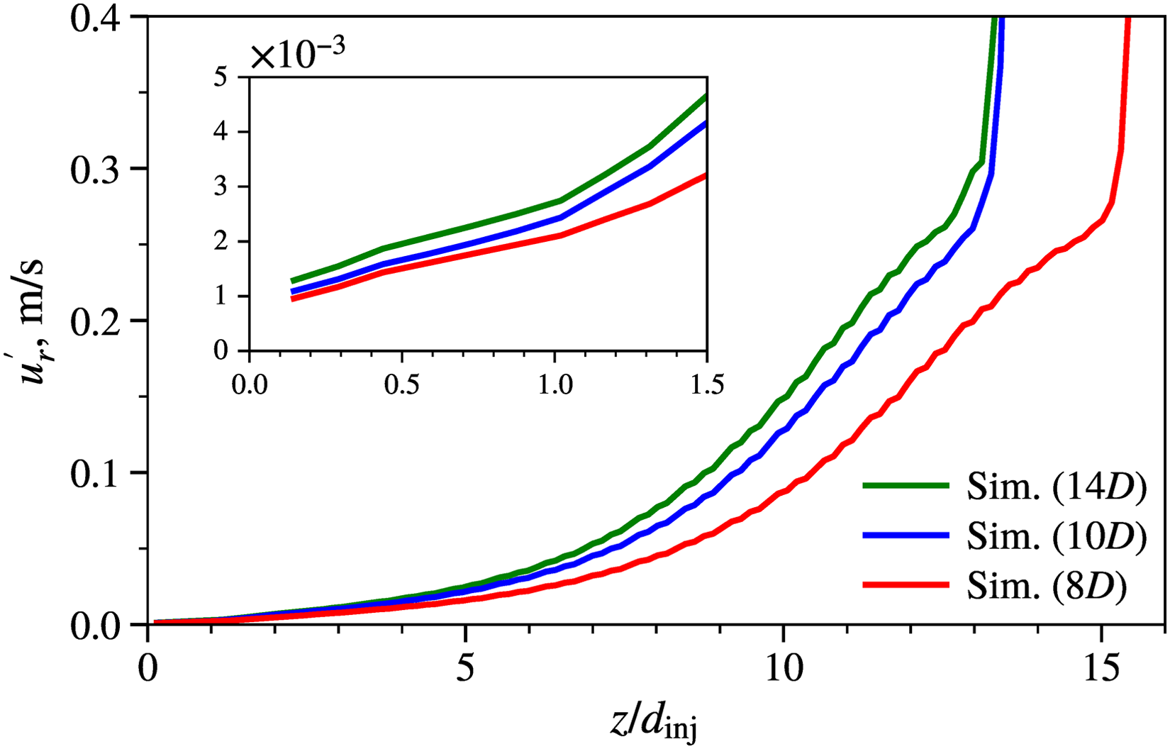
Root-mean-square (RMS) radial velocity (
To quantify the differences in fluctuation magnitude, the RMS radial velocity at
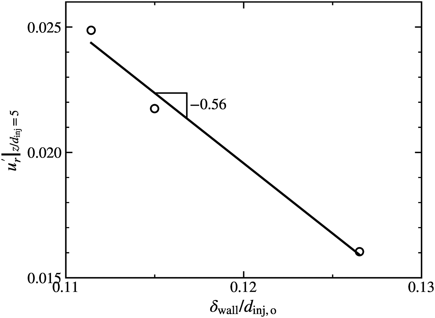
Correlation between the boundary layer thickness at the air-pipe exit (horizontal axis, normalized by the outer diameter of the liquid injector) and the root-mean-square (RMS) radial velocity at
In conjunction with the spray pattern shown in Figure 3, these radial velocity fluctuations are potentially governed by two primary mechanisms: (i) the Kelvin–Helmholtz instability deforms the liquid column into a transverse wave, which perturbs the internal streamwise liquid flow in the radial direction, and (ii) the surrounding gas-phase radial motion induced by the recirculation region downstream of the liquid injector, which can push or pull the column laterally. These mechanisms are examined below.
Kelvin–Helmholtz instability
To assess how the boundary layer thickness in the air pipe influences the onset of Kelvin–Helmholtz instability, the downstream evolution of the mean and RMS axial velocity around the liquid column is analyzed in Figure 15. The velocities are sampled as azimuthal averages at
Azimuthal averages of mean and root-mean-square (RMS) axial velocity (
Flow recirculation downstream of the liquid injector
Radial velocity fluctuations within the liquid column are potentially driven by the recirculation zone immediately downstream of the liquid injector as indicated in Figure 3. Figure 16 shows mean and RMS radial velocity sampled analogously to Figure 15. The recirculation is indicated by negative
Azimuthal averages of mean and root-mean-square (RMS) radial velocity (
Returning to Figure 13, before the onset of Kelvin–Helmholtz growth (
Mechanism of liquid-column instability
Based on the above analyses, a thinner boundary layer on the outer wall of the liquid injector at the air-pipe exit results in a steeper velocity gradient along the liquid-column surface, which strengthens Kelvin–Helmholtz instability. This enhanced instability leads to radial velocity fluctuations within the liquid column even before any visible surface waviness develops, while recirculation-induced radial fluctuations play a secondary role in the present configuration.
As shown in Figure 17, the radial velocity fluctuation within the liquid column strongly correlates with the liquid-column length. The 14
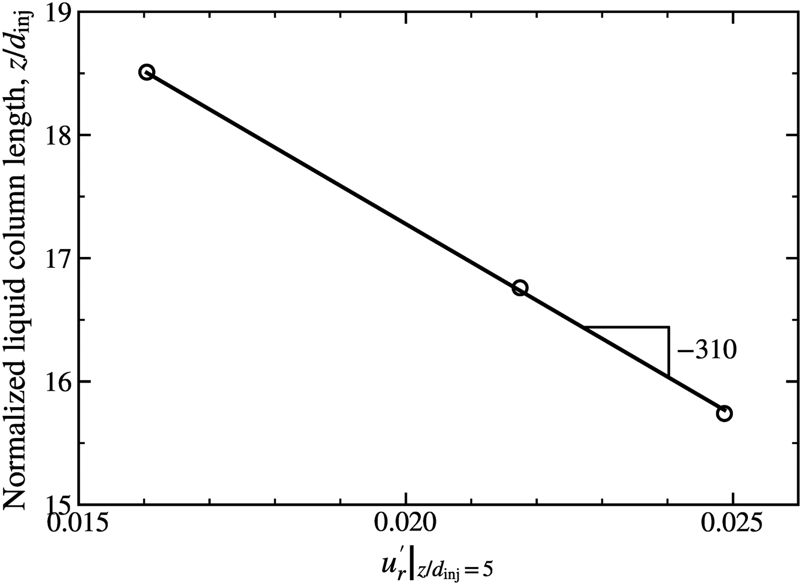
Correlation between the root-mean-square (RMS) radial velocity at
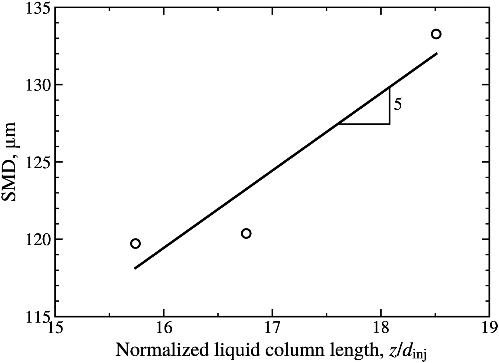
Correlation between the liquid-column length (horizontal axis, normalized by
In summary, one of the key mechanisms governing liquid-column instability and atomization performance in air-assisted atomizers is the boundary layer thickness developed along the outer wall of the liquid injector within the coaxial air pipe. An important finding of this work is that radial velocity fluctuations within the liquid column serve as an indicator of the onset of the liquid-column instability, even before Kelvin–Helmholtz waves become visually noticeable. For practical atomizer design, instability can be enhanced by thinning the boundary layer in the coaxial air pipe through modifications such as increasing the gaseous Weber number and optimizing wall roughness or air-pipe geometry. An alternative approach would be to intensify radial velocity fluctuations within the liquid column, potentially through specialized liquid-injector designs. By inducing these internal perturbations, the liquid core tends to protrude outward from the centerline at earlier axial locations, leading to accelerating primary atomization.
Analysis of atomization process
The simulation captures the atomization process of the spray in the air-assisted atomizer. As the liquid enters the open space, a cylindrical liquid column forms along the centerline (Figure 19). The presence of this column regularizes the previously turbulent gas flow, an effect attributable to a momentum ratio, gas momentum to liquid momentum, of
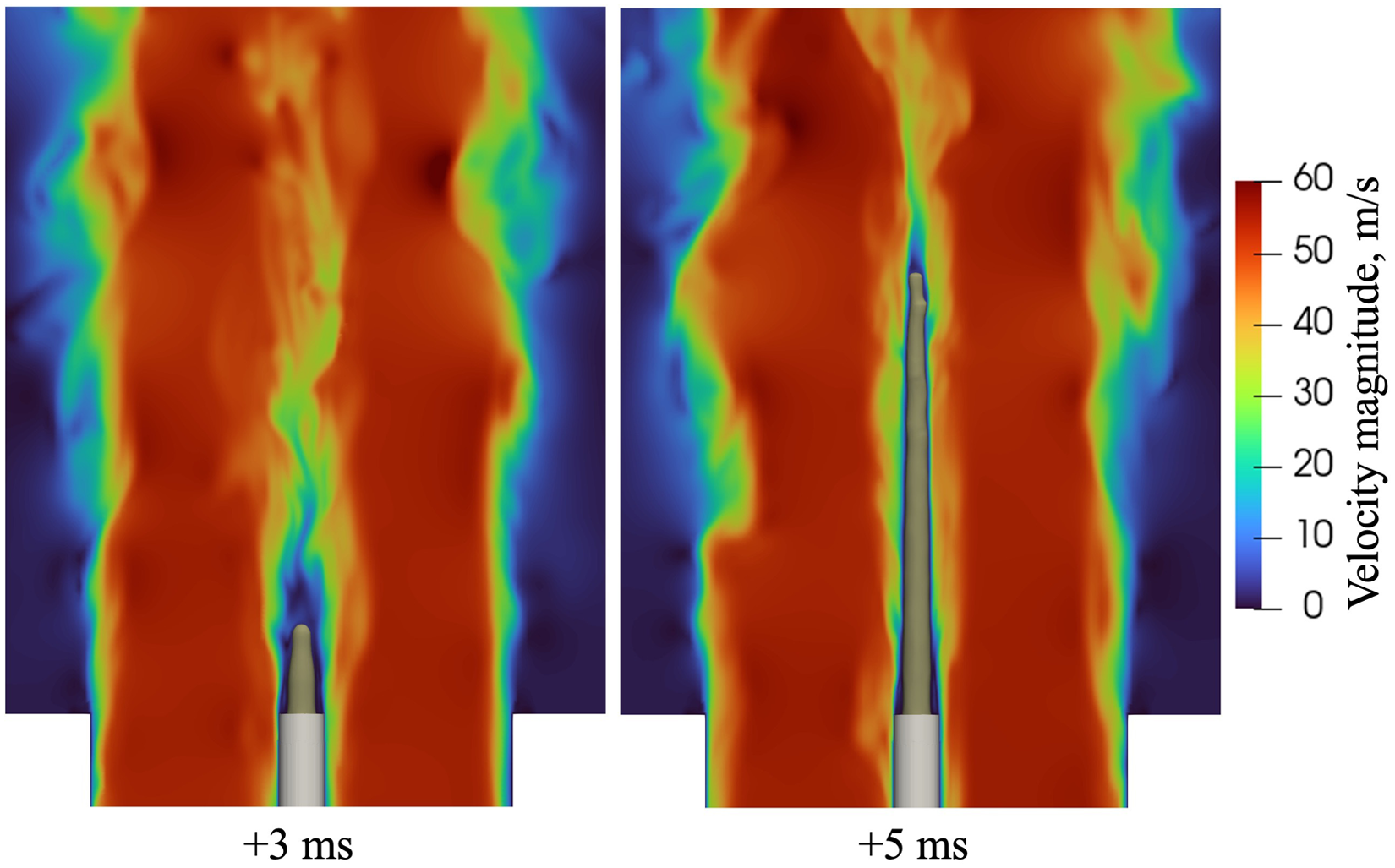
Gas flow regularization by the spray column for the recess 0 mm configuration. Left: gas flow with minimal presence of the liquid column. Right: gas flow with a well-established liquid column, where the cylindrical liquid column regularizes the turbulent gas flow along the centerline. The liquid is shown in dark yellow, the liquid injector in gray, and the colormap represents the gas velocity magnitude.
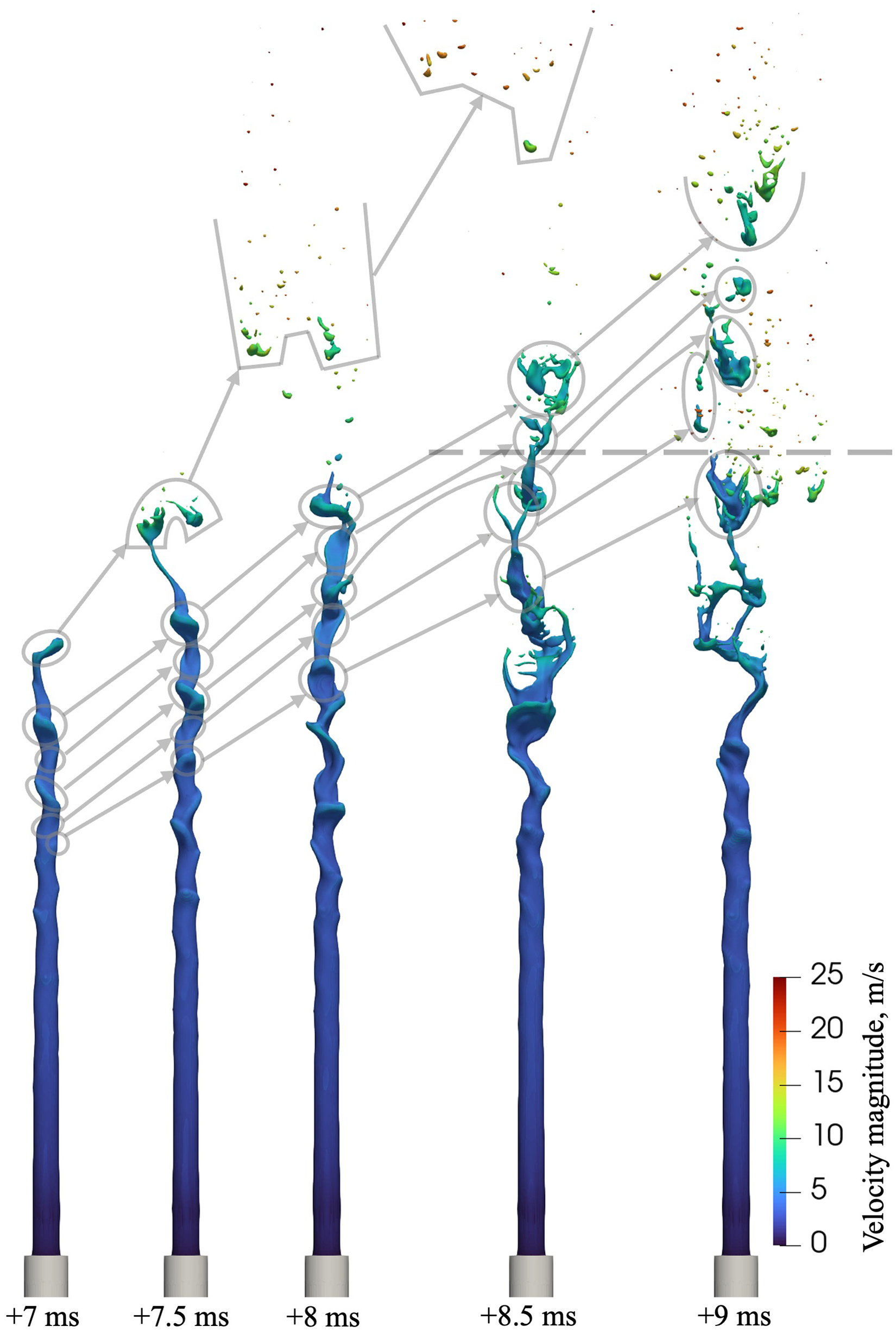
Evolution of spray formation with a colormap representing the velocity magnitude for the recess 0 mm configuration. The arrows trace the evolution of these crests as some of them develop into liquid sheets, then into groups of droplets over time. The dashed line indicates the downstream plane used for the analysis of the liquid mass flow rate.
Figure 21 shows the temporal evolution of the liquid mass flow rate through a downstream plane, indicated by the dashed line in Figure 20. This plane is selected because the liquid sheets have already detached from the liquid column while still retaining a relatively large, coherent structure, prior to fully fragmenting into smaller pieces. As a result, it is well suited for analyzing the intermittent mass-flow bursts associated with these individual large liquid structures.
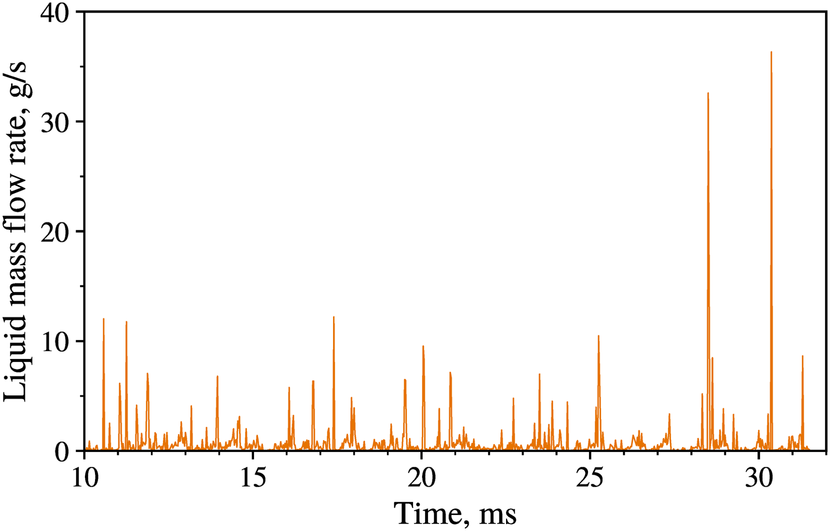
Liquid mass flow rate through a plane located 20 mm downstream of the air-pipe exit for the recess 0 mm configuration. Droplet data are sampled every 0.01 ms and grouped over 0.02 ms intervals.
As illustrated in Figure 20, Kelvin–Helmholtz instability causes each crest on the liquid column to give rise to a group of droplets with a liquid core at the center, and approximately two to three liquid cores pass through the downstream plane every 0.5 ms. This corresponds to a characteristic frequency in the range of 4700–5400 Hz, which forms the dominant frequency band highlighted in red in Figure 22. These frequencies are comparable to the value of
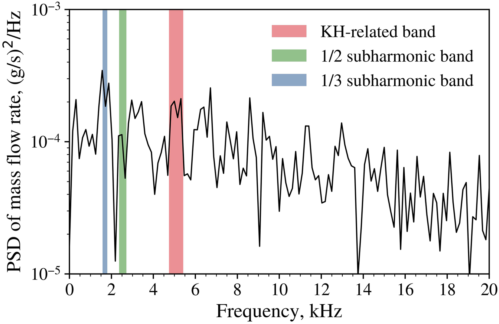
Power spectral density (PSD) of liquid mass flow rate fluctuations through a plane located 20 mm downstream of the air-pipe exit for the recess 0 mm configuration, estimated using Welch’s method. 43 The red band illustrates the Kelvin–Helmholtz-related frequency, while the green and blue bands correspond to the one-half and one-third subharmonic bands, respectively.
Strong dominant low-frequency components in the range of 1600–1800 Hz, highlighted in blue in Figure 22, are of particular interest, as they indicate the presence of pronounced, large-scale unsteady structures generated over axial distances longer than those associated with two successive liquid groups formed by neighboring crests along the liquid column. Notably, these low-frequency components approximately correspond to the one-third subharmonic of the Kelvin–Helmholtz-related frequency band. In addition, less pronounced dominant components, highlighted in green in Figure 22, correspond to the one-half subharmonic of the Kelvin–Helmholtz-related band. Such behavior is physically plausible, as illustrated by the spray evolution in Figure 23. When successive sheets occupy similar radial locations, a downstream sheet can be partially shielded from direct impingement by the high-speed gas due to the presence of an upstream sheet. This shielding reduces the advection speed of the downstream sheet, allowing the upstream sheet to catch up and eventually collide and merge with it. The identification of this subharmonic frequency band and its underlying mechanism provides new insight into air-assisted atomization. To the authors’ knowledge, such behavior has not been reported in the literature.
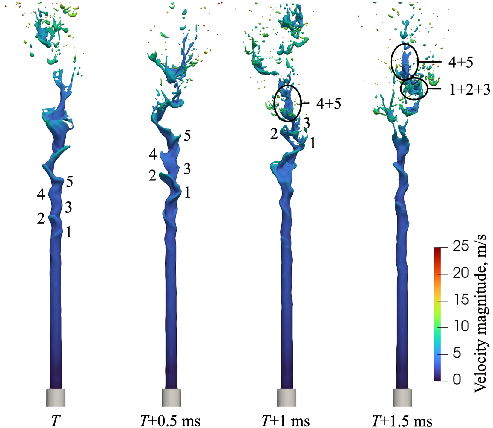
Evolution of liquid-column surface crests (indicated by numbers) at 0.5 ms intervals, showing sheet collision and merger, where
The identification of these frequency modes is potentially valuable for injector design, as they introduce specific characteristic frequencies into the system dynamics. Although the frequency spectrum also depends on factors such as the sampling plane location, the temporal grouping of sampling data, and the segment length used in Welch’s method, the dominant peaks associated with Kelvin–Helmholtz instability and their corresponding subharmonic components remain clearly distinguishable. Future work will focus on developing image-processing techniques to track the temporal evolution of liquid sheets and to quantify the occurrence of events contributing to subharmonic frequencies. Establishing these metrics will provide a more robust and direct link between the frequency spectrum and the underlying sheet-evolution dynamics.
Understanding the atomization process in an air-assisted atomizer, as described above, elucidates the underlying mechanism at the specific
Conclusions
This study presented and validated a high-fidelity numerical framework for atomization in an air-assisted coaxial injector, combining a geometric VOF method with LES and adaptive mesh refinement. Comparison with experimental measurements showed that the simulation accurately captures the mean and fluctuating gas velocities, the divergence point of the liquid column, the characteristic droplet size, and the peak of the droplet size distribution. Some discrepancies remain, however, such as the slight underprediction of liquid presence along the centerline in the far field, prediction of an excessive number of liquid elements smaller than the grid size, and fewer large droplets in the droplet size distribution. To achieve more accurate surface tension forces, future work will adopt RDF-based methods to improve interface curvature estimation. In addition, to mitigate the overprediction of SGS liquid elements, future work will explore transforming such small liquid objects into Lagrangian droplets.
With good agreement in the overall trend of the droplet size distribution relative to the experiment, an assessment of numerical tolerances was performed to investigate their influence on accuracy and computational cost. Even when the tolerances are relaxed relative to those commonly used in fundamental studies, single-droplet tests show that liquid-volume-conservation errors remain negligible over the lifetime of a liquid droplet. Moreover, full spray simulations indicate improved agreement with experimentally measured droplet characteristic sizes, accompanied by a substantial reduction in computational cost. These results suggest that stricter tolerance settings do not necessarily lead to improved accuracy in large-scale spray simulations under the formulations and conditions of the present study.
Varying the coaxial air-pipe length enables investigation of how boundary layer thickness along the outer wall of the liquid injector influences spray dynamics. A thinner boundary layer at the air-pipe exit is strongly correlated with enhanced radial velocity fluctuations within the liquid column, driven by intensified Kelvin–Helmholtz instability due to increased interfacial shear stress. By identifying radial velocity fluctuations within the liquid column as an indicator of the onset of liquid-column instability, the analysis suggests that amplified radial velocity fluctuations can promote earlier breakup of the liquid column, resulting in a shorter intact column and a reduced downstream SMD.
From a physical standpoint, the simulations provide a coherent description of the atomization pathway in an air-assisted injector. After entering the chamber, the liquid forms a cylindrical column that regularizes the core gas flow. High-speed coaxial air excites interfacial waves whose crests stretch into thin sheets that detach, convect downstream, and fragment into ligaments and droplets. The sheet-driven breakup mechanism produces groups of liquid fragments centered around high-inertia liquid sheets, matching one of the dominant frequencies in the intermittent liquid mass flow signals at a downstream sampling location. The corresponding subharmonic frequency components are associated with the collision and merger of successive liquid sheets. This mechanisms responsible for generating specific frequency components in the liquid mass flow rate are potentially valuable for system design, particularly in applications where certain frequencies are undesirable. Overall, the present study establishes a robust numerical framework for modeling sprays in air-assisted atomizers and provides physical insights that advance the design of more efficient atomization and combustion systems.
Footnotes
Acknowledgements
This work was sponsored by the Clean Energy Research Platform at King Abdullah University of Science and Technology (KAUST). Computational resources were provided by the KAUST Supercomputing Laboratory (KSL). ChatGPT was used to assist in improving grammatical flow and clarity in the text.
Funding
The authors disclosed receipt of the following financial support for the research, authorship, and/or publication of this article: The work presented in this article was supported by KAUST.
Declaration of conflicting interests
The authors declared no potential conflicts of interest with respect to the research, authorship, and/or publication of this article.
Appendix A. Solver settings
Appendix B. Sampling liquid elements on a plane
A robust plane-sampling procedure is essential for satisfying two critical criteria: (i) each liquid element is counted only once as it crosses a sampling slab of non-zero thickness and (ii) the time-averaged liquid mass flow rate matches the prescribed target. A slab that is too thick potentially double-counts elements as they advect downstream between successive sampling instants, leading to overestimation. To address this problem, an iterative, thickness-controlled slab is employed, coupled with a de-duplication step based on a liquid-volume tolerance. The algorithm designed to satisfy criteria (i) and (ii) is summarized as follows:
The above procedure does not guarantee that all traversing elements are captured if the slab is too thin relative to the sampling interval and the highest element velocities. To avoid this under-sampling problem, choose the sampling interval short enough that even the fastest liquid elements cannot traverse the slab between two consecutive samples.