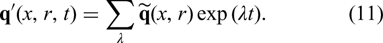
Amplification of perturbations in a laminar premixed swirl flame with the resolvent analysis

Abstract

The global linear stability of a swirl-stabilized laminar flame is analyzed with a monolithic approach based on linearized reactive flow equations. The computational set-up is axisymmetric with an embedded and spatially resolved swirler model to circumvent the use of ad-hoc swirl profile and fluctuation at the inlet. An input–output analysis reveals that the azimuthal and axial components of inertial waves dominate the contribution of inertial waves in gain modulation at low and high frequencies, respectively. A resolvent analysis then identifies the optimal amplification mechanism, which is found to correspond to the flame angle oscillation mechanism observed in experiments. The large gain separation explains why this optimal mechanism also appears in experiments or simulations with acoustic forcing at the inlet. Finally, flame displacement is correlated with radial velocity fluctuations at the base of the flame, which are quasi-normal to the flame sheet. This component of the fluctuating velocity is amplified along the flame sheet until it reaches its tip only if flame-flow feedback is active.

Keywords

thermoacoustic instabilities resolvent analysis swirl-stabilized flames laminar

Introduction

Swirl-stabilized flames are widely used in premixed combustion applications because, upon sufficient swirl intensity, the rotating jet of fuel/air premixture breaks down as it expands into the combustion chamber and thereby generates a central recirculation region downstream. This recirculation region provides a hydrodynamic anchoring point for the flame and the mixing of hot combustion products with the fresh mixture of reactants. The rotating motion of the fluid is generated by a swirler upstream of the combustion chamber, which converts axial or radial momentum into azimuthal momentum, in the case of an axial or a radial swirler, respectively.

Acoustic waves that impinge on the swirler blades generate fluctuations of azimuthal velocity ( ${\hat{u}}_{θ}^{s w}$ in Figures 1 and 2) due to momentum conservation, a process known as mode-conversion.¹ Komarek and Polifke² have shown that such “swirl fluctuations” are transported by convection toward the flame, where they perturb—generally in superposition with fluctuations of velocity, equivalence ratio or vorticity—the flame sheet and the rate of heat release. Fluctuations of heat release rate (HRR) produce acoustic waves, hence closing a potentially unstable thermoacoustic feedback loop.³ Thermoacoustic instabilities impair the development of low-NOx lean premixed combustion devices.⁴

Figure 1.

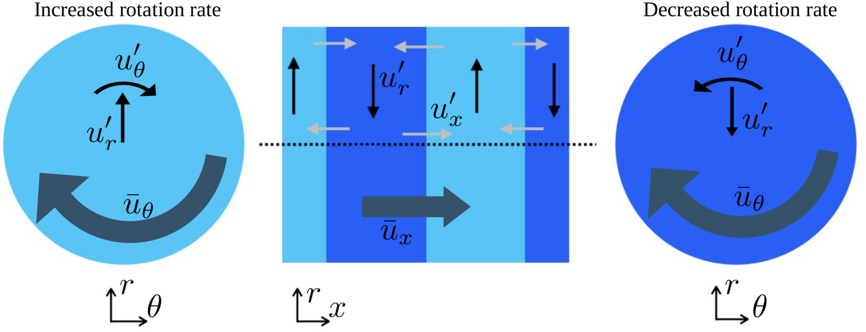
Coupling between velocity components of inertial waves.

Figure 2.

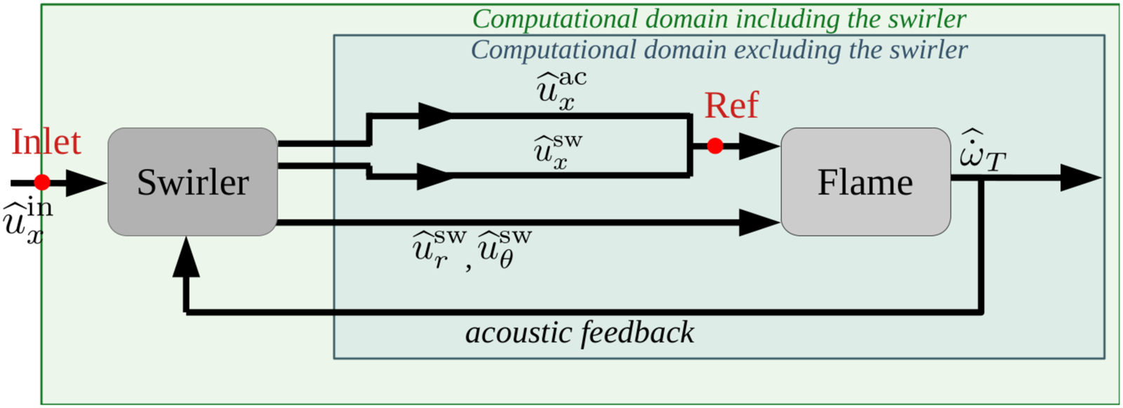
Block diagram representation of the fully-coupled system. The location of the positions “Inlet” and “Reference” is indicated on Figure 3.

Swirl-stabilized flames often exhibit rotational symmetry. In this case, azimuthal velocity fluctuations cannot directly modulate the flame surface, as they are – contrary to axial and radial fluctuations—tangential to the flame sheet. However, some indirect pathways of interaction between swirl fluctuations and HRR have been proposed. Hirsch et al.⁵ proposed that azimuthal vorticity generated by swirl fluctuations modulates the flame surface. Palies et al.¹ and Durox et al.⁶ suggested that swirl fluctuations reaching the base of the flame change the flame angle by changing the radial pressure gradient. This modifies the flame surface and the HRR. Acharya and Lieuwen⁷ investigated a transfer of azimuthal momentum to axial and radial velocity components by a tilting of the vortex core driven by azimuthal velocity fluctuations. This pathway involves non-linear couplings and non-axisymmetrical fluctuations.

More recently, Albayrak et al.^8–10 argued that swirl fluctuations should be properly regarded as inertial waves, which carry axial and radial velocity fluctuations ( ${\hat{u}}_{x}^{sw}$ and ${\hat{u}}_{r}^{sw}$ on Figure 2), in addition to the azimuthal component. As explicated by Greenspan,¹¹ the coupling between azimuthal, axial, and radial velocity fluctuations in inertial waves results from an interplay of Coriolis and centrifugal forces when viewed in the frame of reference attached to the swirling flow: A fluid element located in a rotating slab whose rotation rate, that is, its azimuthal component, is momentarily increased, experiences an increased centrifugal force, which moves this element outside (see the outward-pointing radial component in the light blue slab of Figure 1). Due to the Coriolis effect, this fluid element reduces its rate of rotation (see the dark blue slab in Figure 1). The centrifugal force is thus reduced, and the fluid element moves back to its initial radius. During that inward motion, the rotation rate of the fluid element increases again due to the Coriolis effect. Overall, the column of rotating fluid presents alternating slabs of increased and decreased rotation rates. However, for this sequence of radial motions to fulfill mass conservation at low Mach number, that is, with a scale separation between acoustic and convective wavelength, axial mass flow is required at the inner and outer radii to balance the mass flowing radially inward and outward, hence the axial component (light gray arrows in Figure 1).

Albayrak and Polifke⁹ showed that the speed of propagation of inertial waves in a swirling jet is of the order, but not necessarily equal to the speed of convection, thus providing an explanation of corresponding experimental observations.^2,12,13 More importantly, by time-integrating the low-Mach linearized Navier–Stokes equations, Albayrak et al.¹⁰ demonstrated that the axial and, in particular, the radial velocity components of inertial waves can directly perturb flame surface area and HRR of a laminar, swirl-stabilized flame.¹⁰ Idealized inlet boundary conditions for the base flow and swirl fluctuations at the inlet relied on the mode shapes of inertial waves derived earlier.⁹ In a follow-up study, analytical results for the mode shapes and propagation speeds of inertial waves for a uniform and inviscid rotating flow column were derived.⁸ Varillon et al.¹⁴ confirmed the existence of the axial and radial components on a turbulent swirling jet representative of combustion application.

Albayrak et al.^8–10 and Varillon et al.¹⁴ relied on linear stability analysis, that is, the analysis of the operator driving the evolution of first-order perturbations around a mean- or base-flow. Compared to CFD simulations, which aim at computing the temporal evolution of a system from a specific initial condition or subject to external forcing at its boundary, linear stability analysis provides further insights, such as the prediction of the system’s stability, or identifying the optimal amplification mechanisms.

In the above-mentioned studies, the flow was considered incompressible or “weakly in compressible,” that is, density in a low-Mach-number flow depending only on temperature. In addition, the swirler was excluded from the computational domain. Hence, an ad-hoc azimuthal velocity component, and ad-hoc swirl fluctuations had to be imposed at the input of the computational domain (blue box on Figure 2). But choosing boundary conditions representative of the velocity field downstream of a swirler is challenging. Excluding the swirler from the computational domain also excludes the generation of inertial waves and swirl fluctuations from the feedback loop. The reason why the swirler section has been excluded from all linear stability analyses so far is that its intrinsic three-dimensional nature conflicts with the prohibitive cost of three-dimensional operator-based analyses.

This issue is circumvented by Varillon et al.,¹⁴ who includes the swirler section in the computational domain by using the realistic axisymmetric swirler model of Kiesewetter et al.¹⁵ (green box in Figure 2). This model reproduces the axisymmetric static and dynamic flow fields downstream of a swirler. In this way, the inlet of the flow domain can be moved to a position upstream of the swirler, and is accurately modeled by a developed, non-swirling flow profile. Consequently, there is no need to use idealized boundary conditions, which paves the way to identifying the role of the swirler in the feedback loop.

In the present work, we combine this integrated approach for the swirler with the linearized reactive flow (LRF) model,^16,17 a fully coupled model that studies the global linear stability and amplification of a reactive, compressible flow, excluding ad hoc models for the flame dynamics. As a result, we obtain a monolithic (From Greek monos = single and lithos = stone, that is, “cut from a single stone,” not composed of separate parts ….) framework for global stability of laminar swirling flames. We use this framework to bring a comprehensive understanding of the role of inertial waves in the flow-flame dynamics—from its generation to the action on the flame—via a global linear analysis and resolvent analysis of a model reactive compressible swirling flow.

This article is organized as follows: The configuration of interest and the modeling are presented in Section “Configuration and modeling.” The system’s dynamic is first investigated via three transfer functions identified from an input–output analysis (Section “Flame response”). A resolvent analysis then extends these results, revealing the optimal amplification mechanisms and correlating flame displacement with swirl fluctuations and the velocity field (Section “Amplification mechanisms”).

Configuration and modeling

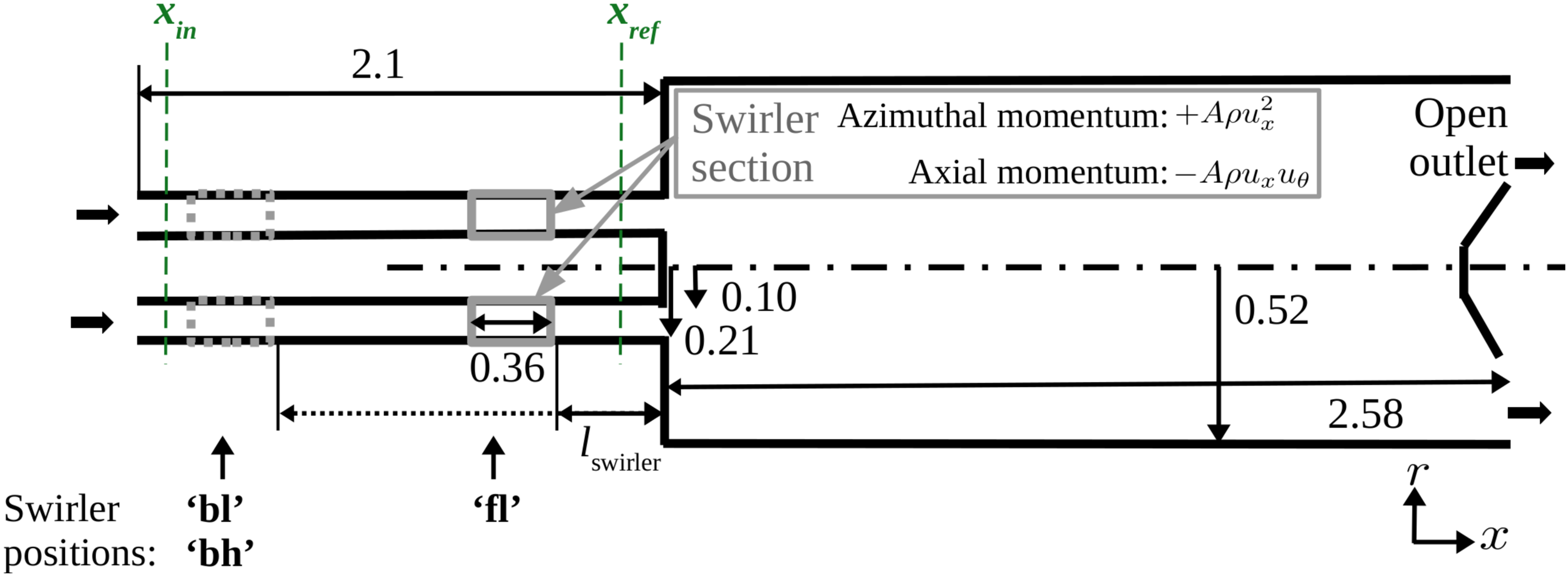
The configuration of interest comprises an annular mixing duct at $Re = 700$ , including a swirler section, that ends in a combustion chamber where a laminar, lean premixed methane flame ( $Φ = 0.8$ ) is stabilized (Figure 3). The dimensions derive from the model flame of Albayrak et al.¹⁰ The system is modeled as a reacting perfect gas of density $ρ$ , sensible enthalpy $h$ , pressure $p$ and velocity $u$ . The evolution equations read:

\partial_{t} ρ + \nabla \cdot (ρ u) = 0,

(1a)

\partial_{t} (ρ u) + \nabla \cdot (ρ u u) + \nabla p = \nabla \cdot τ + Γ,

(1b)

\partial_{t} (ρ h - p) + \nabla \cdot (ρ u h) = \nabla \cdot (λ \nabla T) + {\dot{ω}}_{T},

(1c)

\partial_{t} (ρ Y_{k}) + \nabla \cdot (ρ u Y_{k}) = \nabla \cdot (D_{k} \nabla Y_{k}) + {\dot{ω}}_{k} .

(1d)

The viscous stress

τ

is linked to strain via Stokes’ hypothesis, for which the dynamic viscosity

μ

is obtained from Sutherland’s law. Heat diffusion is modeled with Fourier’s law, with a heat diffusivity

λ

. Heat diffusion due to species of different enthalpies and heating due to viscous friction are neglected compared to the heat-release rate. The combustion of methane is modeled by the two-step BFER reaction mechanism, for which the laminar flame speed and adiabatic flame temperature are verified against the detailed GRI mechanism.¹⁸ Flame dynamics with the BFER is validated by Silva et al.¹⁹ against experiments, based on the flame transfer function of a slit flame. Species are described by their respective mass fraction

Y_{k}

with a reaction rate

{\dot{ω}}_{k} (ρ, h, Y_{k})

; molecular diffusion is described with Fick’s law, with diffusivity

D_{k}

; and HRR is labeled

{\dot{ω}}_{T}

. The swirler is modeled by the coupling term

Γ

, proposed by Kiesewetter et al.,¹⁵ here for an axial swirler,

Γ_{x} = - A (r) ρ u_{x} u_{θ}, Γ_{r} = 0, Γ_{θ} = A (r) ρ u_{x}^{2},

(2)

with

A (r)

a user-defined prefactor, non-zero only in the “swirler section” (Figure 3). This term generates swirl by transferring momentum from the axial to the azimuthal direction while ensuring zero power addition to the flow, as in an actual swirler. This model reproduces experimental axial and azimuthal flow profiles downstream of the swirler.¹⁵ Varillon et al.¹⁴ verified the dynamical behavior of this swirler model by reproducing the dispersion relation of azimuthal velocity fluctuations when forced acoustically upstream. Hence, in addition to producing realistic swirl profiles, this swirler model can also generate inertial waves.

Figure 3.

Configuration of the model burner, describing the two positions of the swirler section (“bl”/“bh” and “fl”). All lengths are non-dimensionalized to the flame length. The positions “Inlet” and “Reference” are reported in green.

The walls are treated as adiabatic no-slip conditions, except the burner back plate, which is cooled to 800 K. A developed annular flow profile at $T_{inlet}$ =293K is enforced at the inlet, and the outlet is stress-free. Equation (1b) is recast into,

\partial_{t} q + L (q) = 0, q = [ρ u h Y_{k}]^{H} .

(3)

The steady state

\bar{q}

of eq. (3) is reached by pseudo time-stepping in the OpenFoam solver reactingFoam for the characteristics given in Table 1,

L (\bar{q}) = 0.

(4)

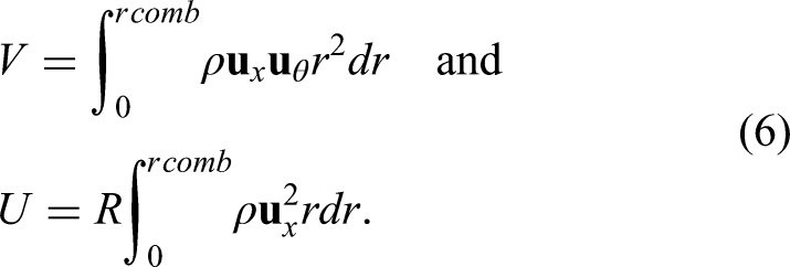
In Table 1, the swirl number is evaluated at the swirler exit as,

S = \frac{V}{U}, with

(5)

\begin{aligned} V = \int_{0}^{r_{comb}} ρ u_{x} u_{θ} r^{2} d r and \\ U = R \int_{0}^{r_{comb}} ρ u_{x}^{2} r d r . \end{aligned}

(6)

The resulting base flow is shown in Figure 4.

Figure 4.

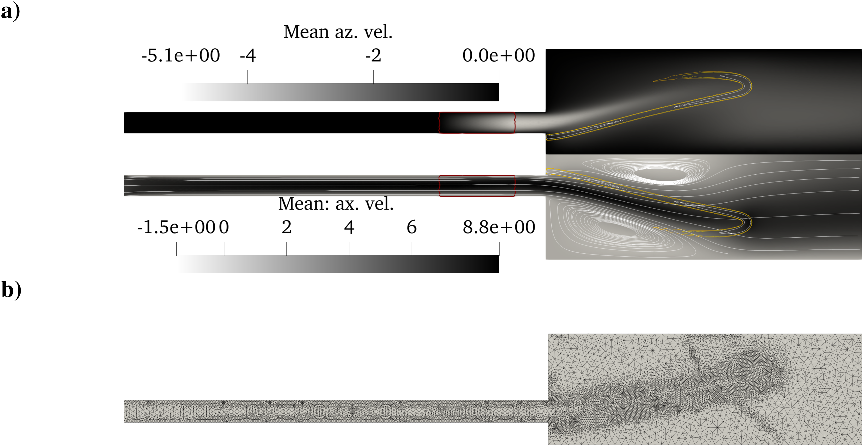
a) Base flow, with the swirler at position 1 and S=0.4. Upper half: ${\bar{u}}_{θ}$ , bottom half: ${\bar{u}}_{x}$ with flow lines. Isocontours: HRR. The swirler section (i.e., non-zero $Γ$ is circled in red. b) Mesh on which the Linearized Reactive Flow equations eq. (13) are discretized.

Table 1.

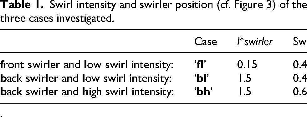
Swirl intensity and swirler position (cf. Figure 3) of the three cases investigated.

	Case	$l *_{swirler}$	Sw
front swirler and low swirl intensity:	‘fl’	0.15	0.4
back swirler and low swirl intensity:	‘bl’	1.5	0.4
back swirler and high swirl intensity:	‘bh’	1.5	0.6

Linear analysis

The flow dynamics is studied through the evolution of small fluctuations around a base state. Each flow variable is split into a mean part $\bar{q}$ , solution to eq. (4), and an infinitesimal fluctuating part $q^{'}$ such that,

q = \bar{q} + ϵ q^{'}, with ϵ ≪ 1.

(7)

The evolution equations for

q^{'}

are obtained by substituting

q

from eq. (7) into eq. (1b) given eq. (4), and then retaining only first-order terms in

ϵ

. First order fluctuations

q^{'}

are governed by,

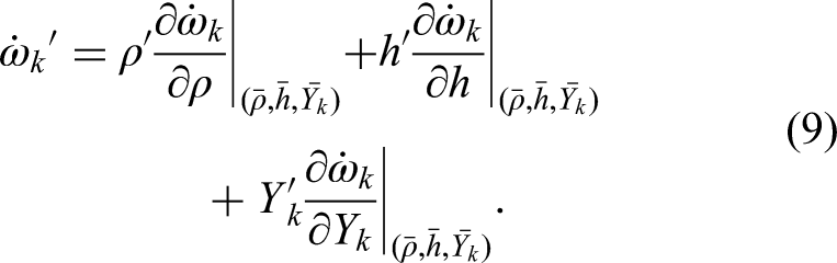
M \partial_{t} q^{'} + L q^{'} = 0, with L = \underset{q}{\nabla} L

(8)

the Jacobian of eq. (1b) and

M

the mass matrix. This equation is referred to as the Linearized Reactive Flow equations (LRF) in the following. Details of the linear operator

L

are given by Meindl et al.,¹⁷ and in particular, the fluctuation of the reaction rate is expressed as

\begin{aligned} {\dot{ω}}_{k}^{'} = ρ^{'} & {\frac{\partial {\dot{ω}}_{k}}{\partial ρ} |}_{(\bar{ρ}, \bar{h}, \bar{Y_{k}})} + h^{'} {\frac{\partial {\dot{ω}}_{k}}{\partial h} |}_{(\bar{ρ}, \bar{h}, \bar{Y_{k}})} \\ + Y_{k}^{'} {\frac{\partial {\dot{ω}}_{k}}{\partial Y_{k}} |}_{(\bar{ρ}, \bar{h}, \bar{Y_{k}})} . \end{aligned}

(9)

The fluctuation of the HRR

{\dot{ω}}_{T}^{'}

follows from the fluctuations of

{\dot{ω}}_{k}^{'}

, as derived in Meindl et al.¹⁷

The strength of LRF lies in providing a monolithic approach to global stability analysis for reactive flow: no ad hoc flame model (e.g., an external flame transfer function) is required, as would be the case in a Helmholtz solver or other hybrid models.

The flame transfer function $F_{r e f}^{({\dot{ω}}_{T})}$ deduced from Equation (8) was validated against experimental results²⁰ and favorably compares against CFD predictions.¹⁶ Based on this validation, LRF is deemed to accurately describe the flame dynamics.

In the latter part of this work, the LRF model is compared against the passive flame model for discussion purposes. The passive flame model uses the base flow solution to eq. (4) but ignores the reaction of the reaction rate to state variable fluctuations by canceling the terms ${\dot{ω}}_{T}^{'}$ and ${\dot{ω}}_{k}^{'}$ in the linearized equations eq. (8).

Equations (1b) and (8) are considered in axisymmetry, i.e., assuming no dependence on the azimuthal coordinate. That is to say, the azimuthal Fourier modes of order greater than 0 are not considered. Likewise, first-order fluctuations of the HRR of azimuthal Fourier modes greater than 0 will cancel once integrated over the volume in the global HRR due to the symmetry of the modes. So, at the first order, non-axisymmetrical perturbations do not participate in the global flame dynamics. The main implication is that the impact of a processing vortex core (PVC) on the flame transfer function is neglected, which was experimentally observed by Durox et al.⁶

The boundary conditions for $q^{'}$ are derived from linearizing the boundary conditions for the base flow. The outlet is non-reflective to acoustic waves. The inlet condition is specified depending on the analysis.

Global linear analysis

Equation (8) is Laplace transformed,

M λ \tilde{q} + L \tilde{q} = 0,

(10)

with

λ

and

\tilde{q} (x, r)

the eigenvalue and eigenvectors. The temporal solution can be reconstructed as,

q^{'} (x, r, t) = \sum_{λ} \tilde{q} (x, r) \exp (λ t) .

(11)

Hence, if at least one eigenvalue has a positive real part, then the flow is linearly unstable, and this associated eigenmode drives the amplification of small perturbations. Otherwise, the flow is globally stable.

Response to harmonic forcing

In the case of a globally stable flow, its response to harmonic forcing can be studied to investigate the amplification process. Equation (8) is Fourier-transformed in time,

2 π i f M \hat{q} + L \hat{q} = \hat{f},

(12)

with

\hat{q} (x, r)

the Fourier coefficients and

\hat{f} (x, r)

a harmonic forcing.

Numerical aspects

Equations (10) and (12) are discretized in space using a DG-FEM scheme¹⁶ on an unstructured grid of 1.7 $\times$ 10 $^{4}$ P1 elements. The resulting linear systems read,

(λ M + L) \tilde{q} = 0 and

(13a)

(2 π i f M + L) \hat{q} = \hat{f},

(13b)

respectively. These linear systems contain 5.3

\times

10⁵ degrees of freedom. For the sake of conciseness, the notations

\tilde{q}

and

\hat{q}

now refers to the spatially discrete eigenvectors and Fourier coefficients, respectively. In the vector notation,

q = [ρ u h Y_{k}]^{t},

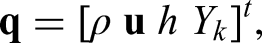
the first element

ρ

now represents a vector block gathering the coefficient of discretized density field, and so on for

u

h

and

Y_{k}

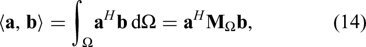
For any vector variables $a$ and $b$ of the same dimensions as $q$ , the scalar product $⟨ a, b ⟩$ is computed as,

⟨ a, b ⟩ = \int_{Ω} a^{H} b d Ω = a^{H} M_{Ω} b,

(14)

where the symmetric matrix

M_{Ω}

represents the mesh quadrature.

Equation (13b) is solved through a MUMPS solver implemented in the PETSc library. Eigenvalues and eigenvectors (eq. (13a)) are computed iteratively via the Krylov–Schur method implemented in the SLEPc library dedicated to solving sparse large eigenvalue problems.²¹

Flame response

This section explores flame dynamics for three cases described in Table 1 and Figure 3: front swirler and low swirl intensity (fl), back swirler and low swirl intensity (bl), and back swirler and high swirl intensity (bh).

Methodology

LRF may used to compute in an efficient and accurate way the laminar flame response to acoustic forcing. An axial inlet velocity perturbation $\hat{f} = {\hat{u}}_{in} = (1, 0, 0)$ is applied to eq. (13). The solution of this equation yields the harmonic response to a velocity forcing at frequency $f$ . The flame transfer function $F_{ref}^{({\dot{ω}}_{T})}$ is then computed at selected frequencies $f$ as,

F_{ref}^{({\dot{ω}}_{T})} (f) = \frac{\int_{Ω} {\hat{\dot{ω}}}_{T} d Ω}{\int_{Ω} {\bar{\dot{ω}}}_{T} d Ω} / \frac{\int_{r_{in}}^{r_{out}} {\hat{u}}_{x, ref} r d r}{\int_{r_{in}}^{r_{out}} {\bar{u}}_{x, ref} r d r},

(15)

with the axial velocity fluctuations

{\hat{u}}_{x}

measured at the reference plane located at the mixing duct exit, i.e., downstream of the swirler (Figure 2). Frequencies are scaled to the flame characteristic convective time

τ_{f}

, i.e., the convection time from the base to the flame tip, such that

f * = f τ_{f}

. Lengths are scaled to the flame length

L_{f}

, such that

l * = l / L_{f}

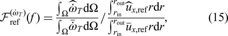
The flame transfer function $F_{ref}^{({\dot{ω}}_{T})}$ is compared against the “system transfer function” $F_{in}^{({\dot{ω}}_{T})}$ ,

F_{in}^{({\dot{ω}}_{T})} (f) = \frac{\int_{Ω} {\hat{\dot{ω}}}_{T} d Ω}{\int_{Ω} {\bar{\dot{ω}}}_{T} d Ω} / \frac{\int_{r_{in}}^{r_{out}} {\hat{u}}_{x, in} r d r}{\int_{r_{in}}^{r_{out}} {\bar{u}}_{x, in} r d r},

(16)

which relates HRR fluctuations to inlet velocity fluctuations, i.e., accounting for the effect of the swirler (Figure 2).

To link the flame and system transfer functions, the “swirler transfer functions” ( $F_{in}^{(u_{)}}$ ) is defined as,

F_{in}^{(u_{a})} (f) = \frac{\int_{r_{in}}^{r_{out}} {\hat{u}}_{a, ref} r d r}{\int_{r_{in}}^{r_{out}} {\bar{u}}_{a, ref} r d r} / \frac{\int_{r_{in}}^{r_{out}} {\hat{u}}_{x, in} r d r}{\int_{r_{in}}^{r_{out}} {\bar{u}}_{x, in} r d r},

(17a)

for the axial and azimuthal component (i.e.,

a = x,

θ

) and,

F_{in}^{(u_{r})} (f) = \int_{r_{in}}^{r_{out}} {\hat{u}}_{r, ref} r d r / \int_{r_{in}}^{r_{out}} {\hat{u}}_{x, in} r d r .

(17b)

F_{in}^{(u_{)}}

quantifies the amplification of axial, radial, and azimuthal velocity fluctuations through the swirler.

Results

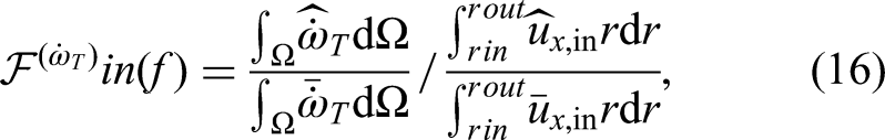
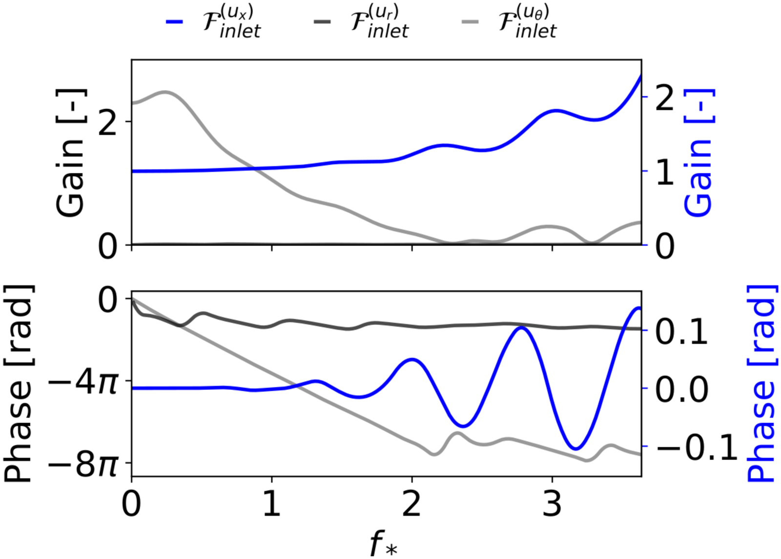
The $F_{ref}^{({\dot{ω}}_{T})}$ matches the low- and high-frequency limits expected for premixed flames, i.e., $F_{ref}^{({\dot{ω}}_{T})} (0) = 1$ and $| F_{ref}^{({\dot{ω}}_{T})} (f) | \to 0$ as $f \to \infty$ (Figure 5).

Figure 5.

$F_{ref}^{({\dot{ω}}_{T})}$ (solid) and $F_{in}^{({\dot{ω}}_{T})}$ (dashed).

At the inlet, acoustic axial velocity fluctuations are imposed on a non-swirling flow ( $u_{x}^{in}$ on Figure 2); therefore, $u_{x}^{in}$ corresponds to acoustic-only fluctuations. These acoustic fluctuations propagate through the swirler and generate an inertial wave that transports velocity fluctuations with azimuthal, radial, and axial components, as demonstrated by Albayrak et al.⁸ for an idealized flow and quantified for a realistic flow by Varillon et al.²² Consequently, at the injector exit downstream of the swirler (at $x_{ref}$ on Figure 2), the fluctuating axial velocity $u_{x}^{'}$ is a superposition of contributions from acoustic fluctuations and the axial component of inertial waves, which cannot readily be distinguished from each other. These two contributions interfere constructively or destructively on the axial velocity. Therefore, the flame and system transfer functions $F_{ref}^{({\dot{ω}}_{T})}$ and $F_{in}^{({\dot{ω}}_{T})}$ give two different points of view on the system: inertial waves are generated upstream of the system, represented by $F_{ref}^{({\dot{ω}}_{T})}$ , but within the system, represented by $F_{in}^{({\dot{ω}}_{T})}$ .

From the low frequency to $f * \approx 1.5$ , the two transfer functions $F_{ref}^{({\dot{ω}}_{T})}$ and $F_{in}^{({\dot{ω}}_{T})}$ are equal for all cases, see Figure 5. In addition $F_{in}^{(u_{x})}$ is approximately 1, so ${\hat{u}}_{x, in} \approx {\hat{u}}_{x} |_{ref}$ , which is consistent with the relation $F_{ref}^{({\dot{ω}}_{T})} F_{in}^{(u_{x})} = F_{in}^{({\dot{ω}}_{T})}$ . Hence, there is no significant contribution of the axial component of the inertial wave on the velocity field at the “ref” location. In that frequency range, the gain of $F_{in}^{(u_{θ})}$ is also significant. Therefore, the azimuthal component dominates the contribution of the inertial wave to the flame response and drives gain modulation of $F_{ref}^{({\dot{ω}}_{T})}$ and $F_{in}^{({\dot{ω}}_{T})}$ at low frequencies. This corresponds to the branch ${\hat{u}}_{θ}$ of the diagram Figure 2.

At higher frequencies, $| F_{in}^{({\dot{ω}}_{T})} |$ > $| F_{ref}^{({\dot{ω}}_{T})} |$ for all three cases. Since the numerators of $F_{ref}^{({\dot{ω}}_{T})}$ and $F_{in}^{({\dot{ω}}_{T})}$ are identical, and the mean axial velocity is unchanged from the inlet to the mixing duct due to mass conservation, we conclude that at higher frequencies,

| \int_{r_{in}}^{r_{out}} {\hat{u}}_{x, ref} r d r | > | \int_{r_{in}}^{r_{out}} {\hat{u}}_{ref} r d r |,

(18)

which is consistent with swirler transfer function

| F_{in}^{(u_{x})} |

rising above 1. The gain of

F_{in}^{(u_{x})}

is also modulated in frequency, which denotes an interference of the axial component of the inertial wave with the acoustic field on

{\hat{u}}_{x}

downstream of the swirler, here measured at

x = x_{ref}

. Simultaneously,

| F_{in}^{(u_{θ})} |

drops. Therefore, the dominant component of inertial waves in its interaction with the flame transitions to its axial component. This corresponds to the branch

{\hat{u}}_{x}

of the diagram Figure 2.

Modeling the oscillations of the transfer functions

The modulations in gain and phase of the swirler transfer function $F_{in}^{(u_{x})}$ can be explained by considering the case of an acoustic and an inertial wave emitted at the same location and oscillating at the same frequency $f_{0}$ , but propagating (in the $x$ direction) at different velocities $c_{ac}$ and $c_{i}$ , respectively. The superposition of these two propagating waves is,

v (x, t) = \sin (2 π f_{0} t - ϕ_{s} (x)) + \sin (2 π f_{0} t - ϕ_{a} (x)),

(19)

with

ϕ_{i} = 2 π f_{0} x / c_{i}

. The amplitude of

v

is then recorded at a position

x_{0}

downstream. The Fourier-transform of the recorded signal

v (x_{0}, t)

reads,

\hat{v} (f) = \int_{- \infty}^{+ \infty} v (x_{0}, t) e^{- 2 π i f t} d t

(20)

\begin{aligned} = & [e^{i \bar{ϕ}} δ (f - f_{0}) - e^{- i \bar{ϕ}} δ (f + f_{0})] \cos (\frac{Δ ϕ}{2}), \end{aligned}

with

\bar{ϕ} = (ϕ_{s} + ϕ_{a}) / 2

and

Δ ϕ = ϕ_{s} - ϕ_{a}

. Retaining only the positive frequencies,

\hat{v} (f) = e^{i \bar{ϕ}} δ (f - f_{0}) \cos (\frac{Δ ϕ}{2}), f > 0.

(21)

In the limit of

c_{ac} ≫ c_{i}

, then

\bar{ϕ} \approx Δ ϕ / 2 \approx ω_{0} x_{0} / (2 c_{i})

. The gain of

\hat{v} (f)

then reads,

| \hat{v} (f) | = δ (f - f_{0}) | \cos (\frac{2 π f_{0} x_{0}}{2 c_{i}}) | .

(22)

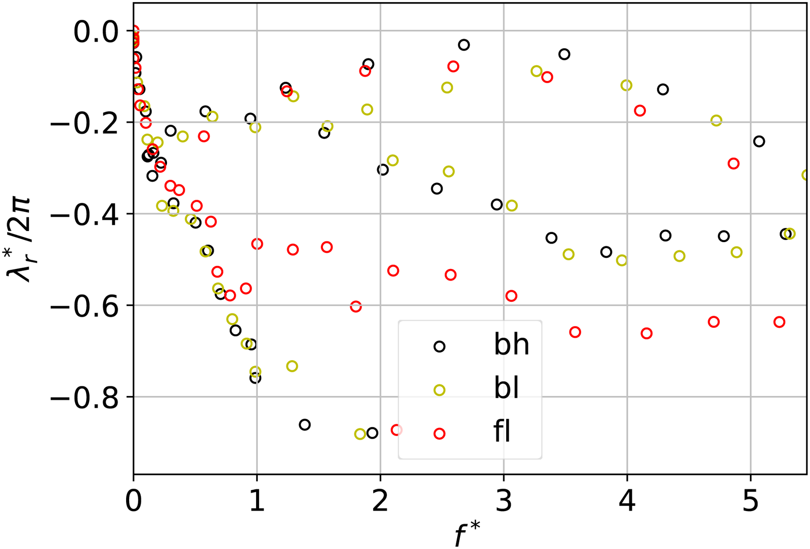
This corresponds to the gain of the monochromatic wave modulated in frequency, with a periodicity

Δ f_{*} = c_{i} / x_{0} .

(23)

The modulation periodicity of

| F_{in}^{(u_{x})} |

from Figure 6 is

Δ f * = 0.74 \pm 0.05

, and the distance of the swirler to the reference plane is

x_{0} * = 1.6

, which gives a corresponding propagation velocity for swirl fluctuations

c_{s} * = 1.2 \pm 0.1

along the duct centerline, i.e., at the maximum base flow velocity or slightly higher.

Figure 6.

Swirler transfer functions (eq. (17a)) for case ‘bh’.

This model is consistent with the signature of axial velocity perturbation transported by inertial waves in the high-frequency range, i.e., for a Strouhal number based on the flame length and bulk flow velocity greater than unity. Hence, the axial component of inertial waves interacts with acoustic waves to shape the gain modulation in the flame response. This further indicates that, in this case, inertial waves propagate preferentially on the fast mode described in Albayrak et al.,⁸ which corroborates experimental evidence that swirl fluctuations propagate faster than the base flow velocity.^2,23

Amplification mechanisms

The investigation of the flame response is now extended by an analysis of the linear operator of eq. (8) driving the first-order fluctuations $q^{'}$ .

The solution to the eigenvalue problem eq. (13a) is computed for non-reflecting inlet and outlet condition. Therefore unstable modes due to reflection at the boundaries are excluded and the targeted amplification mechanisms internal to the system. The spectrum (Figure 7) displays only stable eigenvalues. Therefore, the flow is globally stable and the amplification of small disturbances is driven by the non-normal interaction of the eigenvectors.²⁴ Non-normal interaction of eigenvectors yields transient amplification in the time domain, or equivalently pseudo-resonance of the gain of the resolvent when studied in the frequency domain.²⁵ These mechanisms reveal themselves when the dynamical system eq. (8) is harmonically forced by a body force.²⁶

Figure 7.

Spectrum of the eigenvalue problem eq. (13a) for the three configuration presented in Table 1.

Let $\hat{f}$ be this body force, with components in the axial, radial, and azimuthal directions,

(2 π i f M + L) \hat{q} = \hat{f} .

(24)

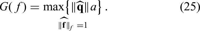
This forcing is applied in the mixing duct. The optimal amplification is the solution to the optimization problem,

G (f) = \underset{‖ \hat{f} ‖_{f} = 1}{max {‖ \hat{q} ‖_{a}}} .

(25)

with

‖ \hat{f} ‖_{\,f}

the

L_{2}

norm of the forcing and

‖ \hat{q} ‖_{a}

a norm, or semi-norm of the response. The index ‘a’ specifies the norm. The resolvent analysis (RA) solves the optimization problem (26) at various frequencies and identifies the optimal gain

G (f)

, associated with the optimal forcing

{\hat{f}}_{opt}

and the optimal response

{\hat{q}}_{opt}

. RA identifies the amplification mechanism that is the most efficient at amplifying small external perturbations.

Equation (25) is recast into,

\hat{q} = R B \hat{f}, with R = {(2 π i f M + L)}^{- 1},

(26)

with

B

an extensor built to impose the forcing

\hat{f}

onto the relevant degrees of freedom. Since the norms (or semi-norms) or the forcing and response derive from scalar products, they can be expressed as quadratic forms of the space-discrete vectors,

‖ \hat{f} ‖_{f}^{2} = {\hat{f}}^{H} Q_{f} \hat{f} and ‖ \hat{q} ‖_{a}^{2} = {\hat{q}}^{H} Q_{a} \hat{q},

(27)

with

Q_{f}

and

Q_{a}

some symmetric (semi-) positive weighting matrices constructed from the mesh quadrature. The superscript

H

indicates the conjugate transpose of a vector or a matrix. With eqs. (27) and (28), eq. (26) is equivalently reformulated as a generalized Hermitian eigenvalue problem,

(R B)^{H} Q_{a} R B \hat{f} = G^{2} (f) Q_{f} \hat{f} .

(28)

The square root of the largest eigenvalue is the optimal gain, and the associated eigenvector is the optimal forcing

{\hat{f}}_{o p t}

. The optimal response

{\hat{q}}_{o p t}

is found by solving the linear system eq. (27) with

\hat{f} = {\hat{f}}_{o p t}

. The subsequent eigenvalues are denominated the suboptimal gains.

Choice of the norm of the response

In the present study, the forcing is restricted to the mixing duct region in order to consider perturbations originating upstream of the flame. Two measures are considered for $‖ \hat{q} ‖_{q}$ :

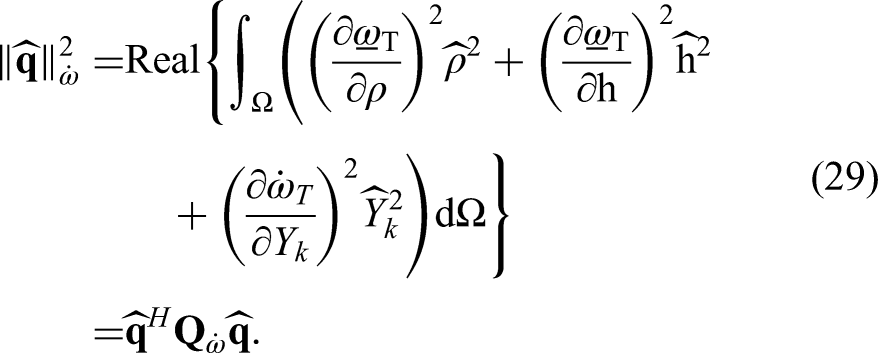
A semi-norm reflecting the HRR fluctuations,

\begin{aligned} ‖ \hat{q} ‖_{\dot{ω}}^{2} = & Real {\int_{Ω} ({(\frac{\partial {\dot{ω}}_{T}}{\partial ρ})}^{2} {\hat{ρ}}^{2} + {(\frac{\partial {\dot{ω}}_{T}}{\partial h})}^{2} {\hat{h}}^{2} \\ + {(\frac{\partial {\dot{ω}}_{T}}{\partial Y_{k}})}^{2} {\hat{Y}}_{k}^{2}) d Ω} \\ = & {\hat{q}}^{H} Q_{\dot{ω}} \hat{q} . \end{aligned}

(29)

The sensitivities of the HRR (

\partial {\dot{ω}}_{T} / \partial q_{i}

relates to eq. (9). This semi-norm does not account for velocity fluctuations.

Chu’s energy,²⁷

\begin{aligned} ‖ \hat{q} ‖_{q}^{2} = & Real {\frac{1}{2} \int_{Ω} (\bar{ρ} {\hat{u}}^{2} + \frac{\bar{c}}{γ} \frac{{\hat{p}}^{2}}{\bar{ρ}} + \frac{\bar{ρ} {\bar{C}}_{v} {\hat{T}}^{2}}{\bar{T}}) d Ω}, \\ = & {\hat{q}}^{H} Q_{Chu} \hat{q} \end{aligned}

(30)

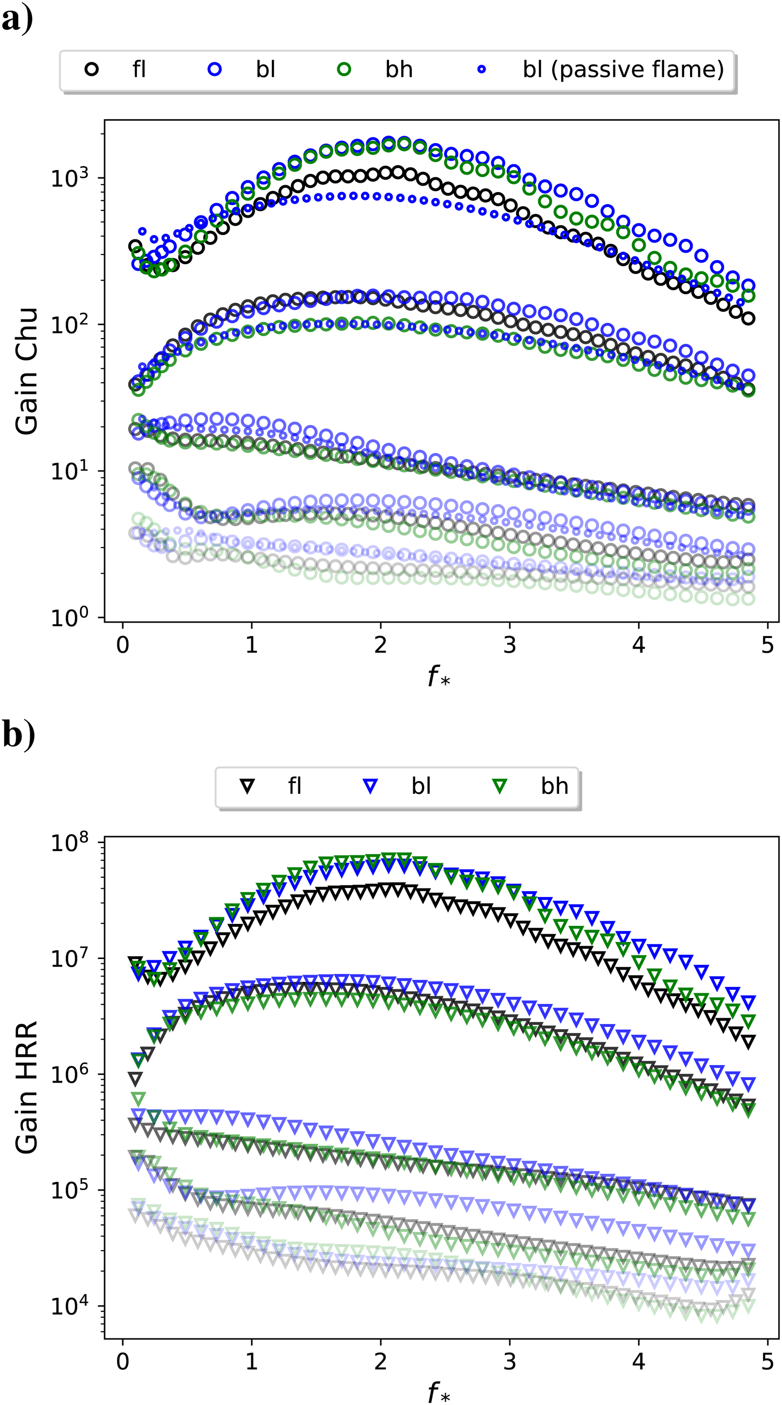
The optimal and suboptimal gain curves are gathered in Figure 8 for the various cases ‘fl’, ‘bl, ‘bh’ (see Table 1) with Chu’s energy as the norm of the response (top), and with the HRR semi-norm (bottom).

Figure 8.

Gains of the resolvent (eq. (26)) for cases ‘fl’, ‘bl’ and ‘bh’: a) norm of Chu, b) HRR semi-norm. Suboptimal gains with increased transparency.

Overall, Chu’s energy and HRR semi-norm exhibit trends that suggest qualitatively similar behavior, although the gain values differ by several orders of magnitude (Figure 8, circles vs. triangles): The clear gain separation between the optimal and the suboptimal gains indicates that a single amplification mechanism dominates the flow-flame dynamics over the entire spectrum. Hence, analysis of the gain curves may be considered independent of the choice of the norm. In the following, we use Chu’s norm.

Optimal responses and flame motions

The section analyses the optimal forcings and responses to link swirl fluctuations to flame motions. The optimal forcing is the perturbation field to which the flame-flow system is the most responsive. The optimal response is the way the system responds to it.

Swirl fluctuations and flame motions

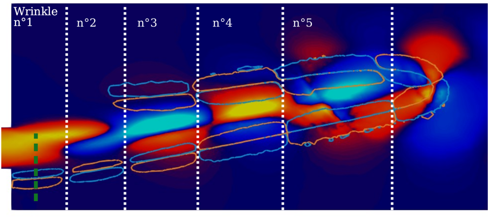
In this section, we investigate the link between swirl fluctuations and flame motion. Flame wrinkles are identified from ${\hat{\dot{ω}}}_{T}$ : the flame is moving out of regions of negative ${\hat{\dot{ω}}}_{T}$ (blue isolines on Figure 9), and toward region of positive ${\hat{\dot{ω}}}_{T}$ (orange isolines). We can then define flame wrinkles moving outward and inward of the V-shape (white dashed lines). Each wrinkle is located between an abscissa $x_{min}$ and $x_{max}$ that can be determined from ${\hat{\dot{ω}}}_{T}$ contours and the white dashed lines (Figure 9).

Figure 9.

Close-up view of the combustion chamber. Heatmap: integrand of eq. (31) (colorbar scaled to [-max;max], deep blue to yellow). Contours: iso- $ℜ {{\hat{\dot{ω}}}_{T}}$ fluctuations, negative (light blue) and positive (orange), indicating flame motion. The case is input–output analysis at $f * = 1.75$ , corresponding to Table 3. The slabs corresponding to the flame wrinkles are delimited by the vertical white dashed lines.

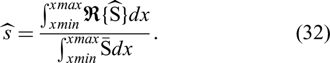
The first order fluctuation of the swirl number at a given location $x$ is stems from the linearization of eq. (6),

\frac{ℜ {\hat{S}}}{\bar{S}} = \frac{ℜ {\hat{V}}}{\bar{V}} - \frac{ℜ {\hat{U}}}{\bar{U}} =

(31)

\begin{aligned} \int_{0}^{r_{comb}} \bar{ρ} {\frac{({\bar{u}}_{x} ℜ {{\hat{u}}_{θ}} + {\bar{u}}_{θ} ℜ {{\hat{u}}_{x}}) r^{2}}{\bar{V}} - \frac{2 R {\bar{u}}_{x} ℜ {{\hat{u}}_{x}} r}{\bar{U}}} d r, \end{aligned}

with

U

and

V

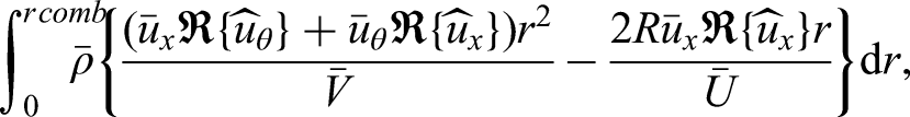
defined in eq. (6). To correlate linear fluctuation of the swirl number and flame motions, the ratio

ℜ {\hat{S}} / \bar{S}

is integrated in the

x

-direction on slabs covering each flame wrinkle,

\hat{s} = \frac{\int_{x_{min}}^{x_{max}} ℜ {\hat{S}} d x}{\int_{x_{min}}^{x_{max}} \bar{S} d x} .

(32)

The sign of

\hat{s}

indicates whether the overall swirl around a specific flame wrinkle increases or decreases compared to

\bar{S}

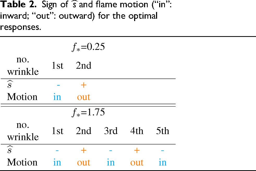
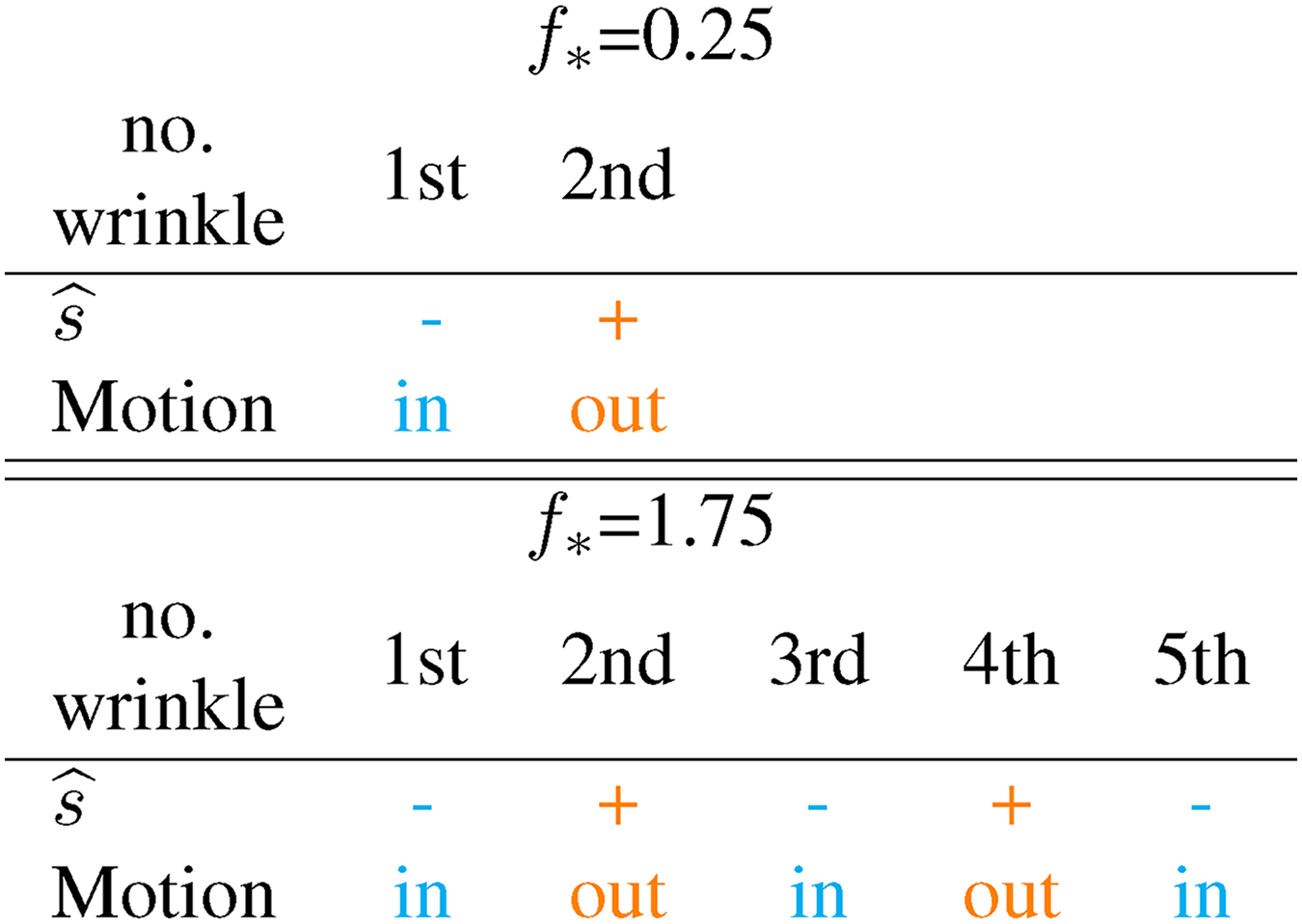
Table 2 displays how local swirl fluctuations and flame wrinkles relate in the optimal response ${\hat{q}}_{opt}$ of the RA. The sign of $\hat{s}$ is not sensitive to a slight change in the white dashed lines delimiting the flame wrinkles (Figure 9). There is a clear correlation between the outward (respectively inward) pointing motion of the flame and positive (rep. negative) swirl number fluctuation. This is valid along the entire flame sheet and at both frequencies presented.

Table 2.

Sign of $\hat{s}$ and flame motion (“in”: inward; “out”: outward) for the optimal responses.

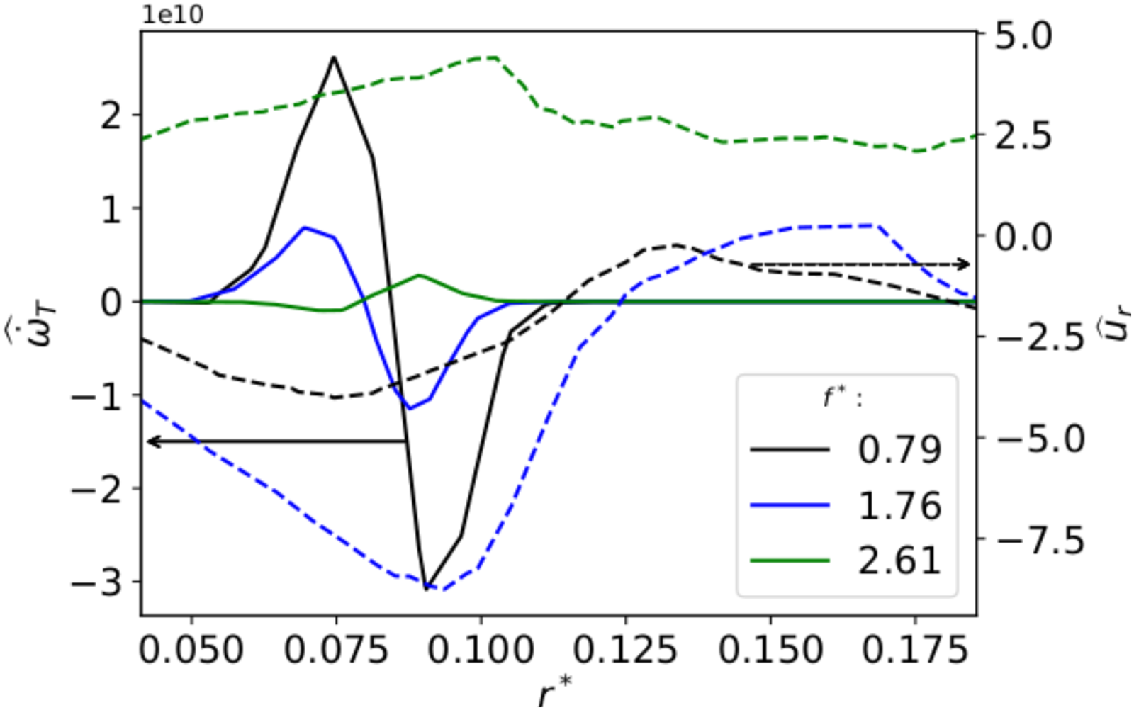
Such a behavior of the optimal response ${\hat{q}}_{opt}$ corresponds to the flame angle oscillation mechanism experimentally identified in Palies et al.²³ and Candel et al.,²⁸ by which swirl fluctuations produce HRR fluctuations: slabs of positive (resp. negative) swirl fluctuations cause a widening (resp. narrowing) of the flame angle that is convected downstream. Figure 10 indeed indicates a correlation of negative (resp. positive) radial velocity fluctuation with an inward (resp. outward) motion of the flame base at three various frequencies: the flame moves away of the region of negative $ℜ {{\hat{\dot{ω}}}_{T}}$ toward regions of positive $ℜ {{\hat{\dot{ω}}}_{T}}$ . This mechanism is combined with vorticity transport, which is another thermoacoustic feedback mechanism not specific to swirl flame. Therefore, the resolvent analysis identifies the flame angle oscillation mechanism experimentally identified by Palies et al.²³ and Candel et al.²⁸ as the most efficient at amplifying small flow fluctuations on this model swirling flame.

Figure 10.

Line plot along the green line on Figure 9 of $ℜ {{\hat{u}}_{r}}$ and $ℜ {{\hat{\dot{ω}}}_{T}}$ for three frequencies. Optimal response of the RA of case ‘bl’ in Table 1.

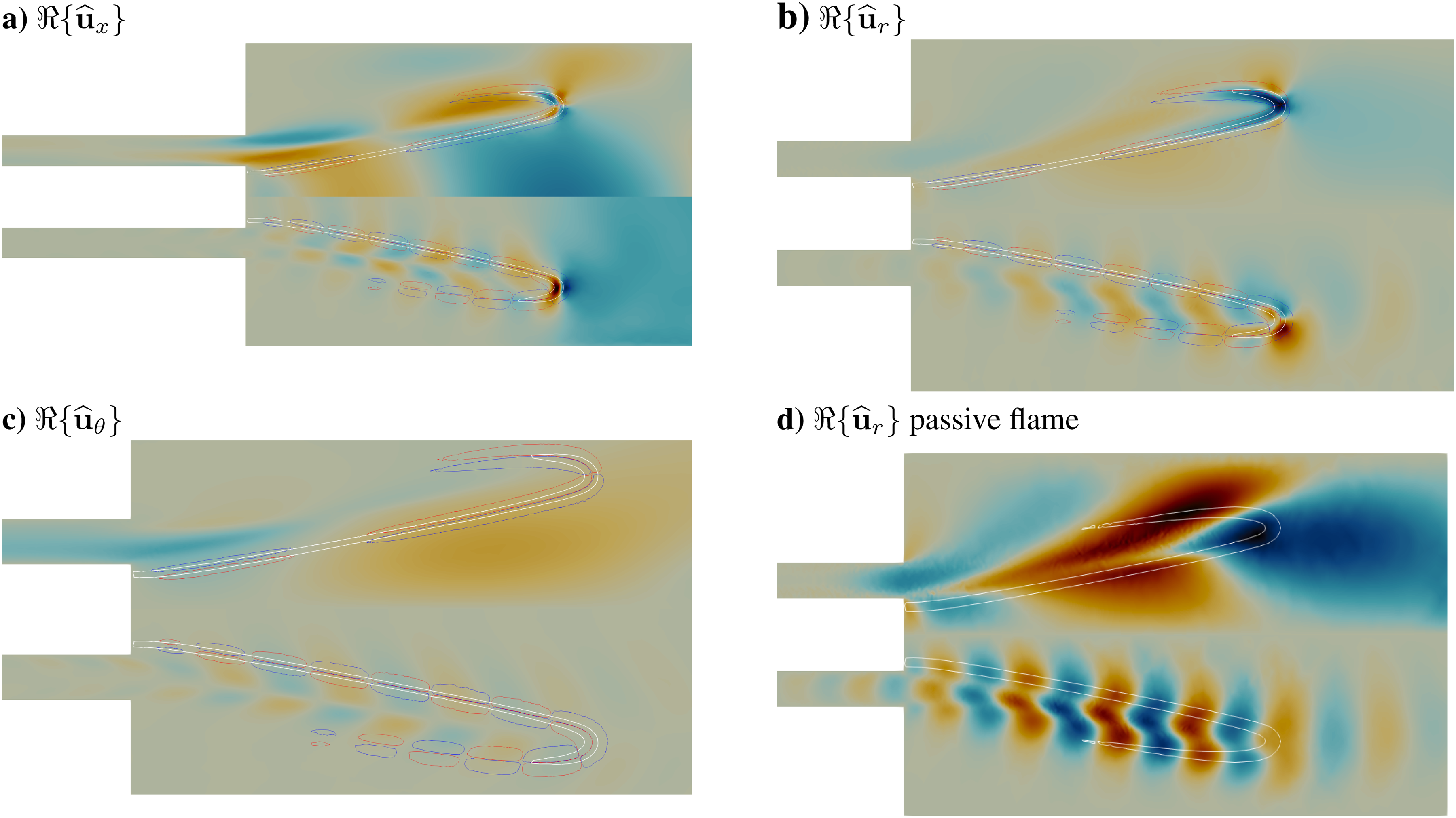
When moving downstream of the flame anchoring, the radial velocity fluctuation is amplified (Figure 11b). The same happens to the axial velocity fluctuation (Figure 11a). Both reach a maximum at the flame tip. On the contrary, the azimuthal velocity fluctuation (Figure 11c) is slightly amplified but decays before the flame tip after a few wavelengths, as for the radial velocity perturbation from the passive flame approach (Figure 11d).

Figure 11.

Case ‘bl’, upper halves: $f_{*}$ =0.24, lower halves: $f_{*} = 2.9$ . White contour: isoline of ${\bar{\dot{ω}}}_{T}$ , colored contour: isoline of $ℜ {{\hat{\dot{ω}}}_{T}}$ , blue for negative, red for positive values. Blue-orange heatmap: optimal responses of a) $ℜ {{\hat{u}}_{x}}$ , b) $ℜ {{\hat{u}}_{r}}$ and c) $ℜ {{\hat{u}}_{θ}}$ , scaled to the maximum of $| ℜ {{\hat{u}}_{i}} |$ , for $i = x$ , $r$ and $θ$ . d) $ℜ {{\hat{u}}_{r}}$ for the passive flame model scaled to its maximum absolute value.

This distinction is attributed to the flame-flow feedback: the fluctuating HRR and the associated fluctuating expansion act on the velocity components non-tangential to the flame sheet ( $u_{x}^{'}$ and $u_{r}^{'}$ ), amplifying them along the flame sheet before it reaches its maximum at the flame tip. This is consistent with the passive flame approach: when the fluctuating HRR is not included in the equations, the perturbed flame cannot act on the flow perturbation through fluctuating flow expansion.

This behavior was already reported in Steinbacher and Polifke²⁹ in the context of G-equation modeling: convective perturbations grow along the flame sheet when flame-flow feedback (named “bidirectional model”) is accounted for. With this feedback, they achieve a better agreement with the flame transfer function computed from CFD than without it. The present work further adds that flame-flow feedback is a key feature of the most efficient amplification mechanism, i.e., the one that is effectively observed in CFD simulations and experiments. Indeed, the optimal gain of the resolvent for the passive flame model is roughly halved compared to LRF (Figure 8a), but the suboptimal gains are not affected.

From optimal forcing to inlet acoustic forcing

However, the velocity forcing applied to swirl flames in experiments^23,28) is an acoustic wave imposed at the inlet, which does not consist of the optimal forcing ${\hat{f}}_{opt}$ identified in Figure 11a. How can the optimal response (Figure 11b-d) then manifest itself? This results from the fact that the optimal response ${\hat{q}}_{opt}$ dominates the suboptimal amplifications by one order of magnitude or more, i.e., the gain separation on Figure 8. Therefore, even if the forcing does not perfectly align with ${\hat{f}}_{opt}$ , the response will be dominated by ${\hat{q}}_{opt}$ , and, understandably, its qualitative behavior shows through experimental or CFD results.

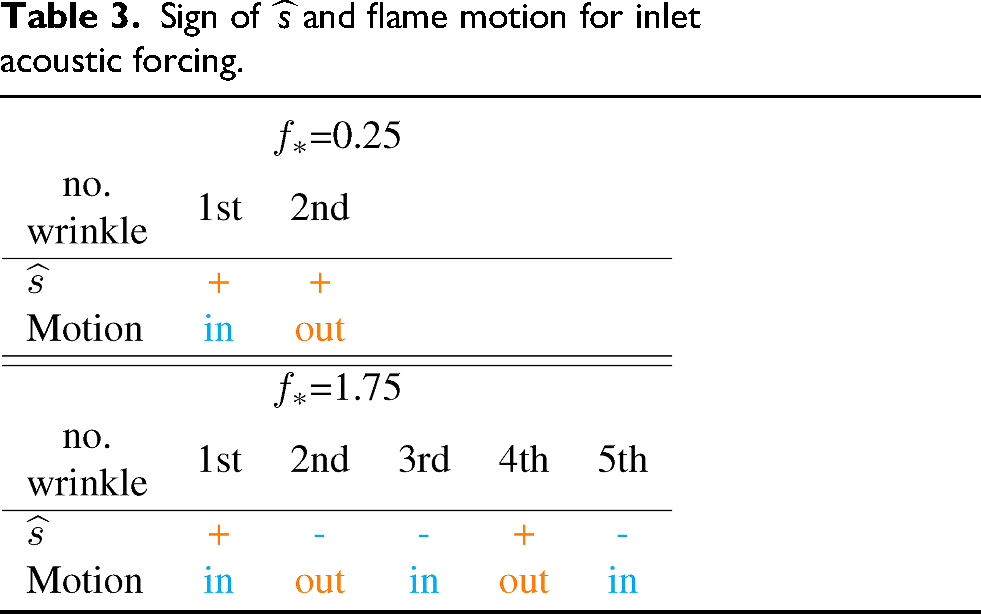
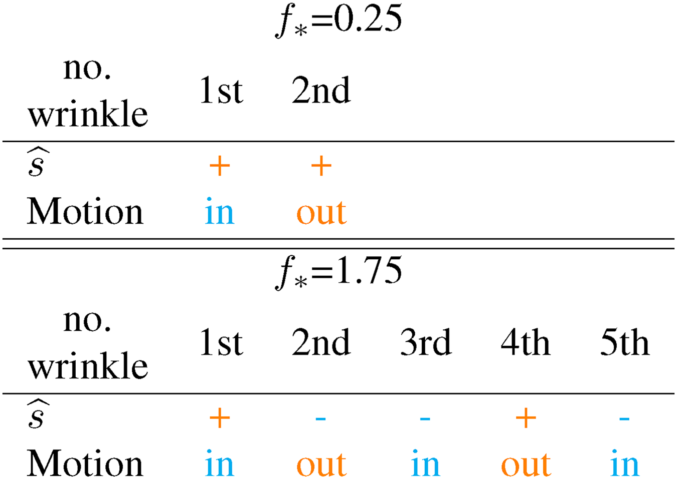
This is what is observed when imposing an inlet axial velocity forcing on eq. (8): the response only shows a correlation between positive $\hat{S}$ and outward flame motion in the downstream part of the flame, that is, close to the flame tip (Table 3). Since $| {\hat{\dot{ω}}}_{T} |$ is larger close to the flame tip and since the flame surface is more significant at its tip rather than its base due to the V-shape in rotational symmetry, the occurrence of the optimal mechanism in the region producing large HRR fluctuations is enough for it to dominate the response.

Table 3.

Sign of $\hat{s}$ and flame motion for inlet acoustic forcing.

Acoustic forcing at the inlet results in being only partially optimal, meaning that other mechanisms are at play at the base of the flame. These other mechanisms can include the axial component of inertial waves described in Section “Configuration and modeling.” The radial component is too small to be significant (Figure 6).

Conclusion

This work presents a novel monolithic approach to global linear stability of swirl-stabilized flame, embedding the linearized reactive flow equations and an axisymmetrical swirler model in a single computational domain. We thus avoid the use of ad-hoc inlet conditions for the swirl profile and fluctuations.

By comparing the flame, system, and swirler transfer functions, we showed that at low frequencies the gain is driven by the azimuthal component of inertial waves – transporting swirl fluctuations – while the axial component dominates at higher frequencies. In addition, inertial waves propagate preferentially on the fast mode at higher frequencies.

The flow-flame dynamics are further investigated via a resolvent analysis that identifies flame angle oscillations as the most efficient mechanism for amplifying perturbations. This follows from a positive correlation between local swirl fluctuations and outward/inward flame displacement by radial velocity fluctuations. This optimal mechanism is active in the downstream part of the flame, where the HRR response is the highest. The operator displays a high gain separation, which means that this optimal amplification mechanism dominates by far other suboptimal mechanisms and explains why this optimal mechanism appears in experiments of simulations with a mere acoustic forcing at the inlet. Flame-flow feedback is also part of this optimal mechanism, as it amplifies radial and axial velocity fluctuation along the flame sheet.

Footnotes

ORCID iDs

Grégoire Varillon

Wolfgang Polifke

Funding

The authors received no financial support for the research, authorship, and/or publication of this article.

Declaration of conflicting interests

The authors declare no potential conflicts of interest with respect to research, authorship, and publication of this article.

References

Palies

Schuller

Durox

, et al. Modeling of premixed swirling flames transfer functions. Proc Combust Inst 2011; 33: 2967–2974.

Komarek

Polifke

. Impact of swirl fluctuations on the flame response of a perfectly premixed swirl burner. J Eng Gas Turbine Power 2010; 132: 061503.

Ducruix

Schuller

Durox

, et al. Combustion dynamics and instabilities: elementary coupling and driving mechanisms. J Propul Power 2003; 19: 722–734.

Lieuwen

Yang

, editors. Combustion instabilities in gas turbine engines: operational experience, fundamental mechanisms and modeling, volume 210 of Progress in Astronautics and Aeronautics. American Institute of Aeronautics and Astronautics, Reston, VA, USA, 2005. ISBN 978-1-56347-669-3.

Hirsch

Fanaca

Reddy

, et al. Influence of the Swirler Design on the Flame Transfer Function of Premixed Flames. In Volume 2: Turbo Expo 2005, pp. 151–160, Reno, NV, USA, January 2005. ASMEDC. ISBN: 978-0-7918-4725-1 978-0-7918-3754-2. doi10.1115/GT2005-68195.

Durox

Moeck

Bourgouin

J-F

, et al. Flame dynamics of a variable swirl number system and instability control. Combust Flame 2013; 160: 1729–1742.

Acharya

Lieuwen

. Effect of azimuthal flow fluctuations on flow and flame dynamics of axisymmetric swirling flames. Phys Fluids (1994-present) 2015; 27: 105106.

Albayrak

Juniper

Polifke

. Propagation speed of inertial waves in cylindrical swirling flows. J Fluid Mech 2019; 879: 85–120.

Albayrak

Polifke

. Propagation velocity of inertial waves in cylindrical swirling flow. In 23nd Int. Congress on Sound and Vibration (ICSV23), Athens, Greece, 2016. IIAV.

10.

Albayrak

Bezgin

Polifke

. Response of a swirl flame to inertial waves. Int J Spray Combust Dyn 2018; 10: 277–286.

11.

Greenspan

. The theory of rotating fluids. Cambridge: CUP Archive, 1968.

12.

Acharya

Lieuwen

. Role of Azimuthal flow fluctuations on flow dynamics and global flame response of axisymmetric swirling flames. In 52nd Aerospace Sciences Meeting, National Harbor, Maryland, January 2014. American Institute of Aeronautics and Astronautics. ISBN 978-1-62410-256-1. DOI:10.2514/6.2014-0654.

13.

Palies

Durox

Schuller

, et al. Experimental study on the effect of swirler geometry and swirl number on flame describing functions. Combust Sci Technol 2011; 183: 704–717.

14.

Varillon

Kaiser

Oberleithner

, et al. Stability of swirl and jet flames—DFG final report. Abschlußberichte / Final report, DFG, September 2024a.

15.

Kiesewetter

Hirsch

Fritz

, et al. Two-dimensional flashback simulation in strongly swirling flows. In ASME Turbo Expo 2003, Collocated with the 2003 International Joint Power Generation Conference, volume GT2003-38395, Atlanta, GA, USA, 2003. doi/10.1115/GT2003-38395.

16.

Avdonin

Meindl

Polifke

. Thermoacoustic analysis of a laminar premixed flame using a linearized reacting flow solver. Proc Combust Inst 2019; 37: 5307–5314.

17.

Meindl

Albayrak

Polifke

. A state-space formulation of a discontinuous Galerkin method for thermoacoustic stability analysis. J Sound Vib 2020; 481: 115431.

18.

Franzelli

Riber

Gicquel

LYM

, et al. Large of combustion instabilities in a lean partially premixed swirled flame. Combust Flame 2012; 159: 621–637.

19.

Silva

Emmert

Jaensch

, et al. Numerical study on intrinsic thermoacoustic instability of a laminar premixed flame. Combust Flame 2015; 162: 3370–3378.

20.

Varillon

Brokof

Polifke

. Global linear stability analysis of a slit flame subject to intrinsic thermoacoustic instability. In Proceedings of the 29th International Congress on Sound and Vibration. Society of Acoustics, Prague, CZ, September 2023. ISBN 978-80-11-03423-8.

21.

Hernàndez

Romàn

Tomàs

, et al. Krylov-Schur methods in SLEPc. SLEPc Technical Report STR-7, 2007.

22.

Varillon

Kaiser

T-L

Brokof

, et al. Linear analysis of a swirling jet with a realistic swirler model. Int J Spray Combust Dyn 2024b; 16: 186–199.

23.

Palies

Durox

Schuller

, et al. The combined dynamics of swirler and turbulent premixed swirling flames. Combust Flame 2010; 157: 1698–1717.

24.

Trefethen

Reddy

, et al. Hydrodynamic stability without eigenvalues. Science 1993; 261: 578–584.

25.

Schmid

Henningson

. Stability and transition in shear flows. Number 142 in Applied Mathematical Sciences. Springer, New York Berlin Heidelberg, 2001. ISBN 978-1-4612-6564-1 978-0-387-98985-3. doi10.1007/978-1-4613-0185-1.

26.

Farrell

. Developing disturbances in shear. J Atmos Sci 1987; 44: 2191–2199.

27.

Chu

B-T

. On the energy transfer to small disturbances in fluid flow (part 1). Acta Mech 1965; 1: 215–234.

28.

Candel

Durox

Schuller

, et al. Dynamics of swirling flames. Annu Rev Fluid Mech 2014; 46: 147–173.

29.

Steinbacher

Polifke

. Convective velocity perturbations and excess gain in flame response as a result of flame-flow feedback. Fluids 2022; 7: 61.