
Abstract
Reliable and computationally efficient prediction capabilities for combustion instabilities in liquid propellant rocket combustion chambers are still rare. This study uses a low-order tool based on the well-known acoustic network model principle to map the stability limits of two different research rocket combustors with different cryogenic propellant combinations. New elements were derived capable of describing any isentropic background flow field in a contoured chamber, resolving acoustic chamber modes in three dimensions, and supporting distributed flame response models. Furthermore, an improved boundary condition element for the sonic throat of a rocket nozzle was implemented. The new network elements were benchmarked against two different research rocket combustion chambers, one single injector experiment using liquid oxygen and natural gas, exhibiting longitudinal mode instabilities and one multi-element thrust chamber with transverse mode instabilities. The acoustic resonant frequencies are predicted with an average absolute error of less than 5% for both cases. The tool is capable of predicting stability based on classical time lag and gain parameters applied to the new distributed flame model. The resulting stability maps are consistent with the benchmark cases for flame response time lags which are close to those reported in literature from computational fluid dynamics simulations and experiments.
Keywords
Introduction
High-frequency (HF) combustion instabilities present a high risk for the development and testing of liquid-propellant rocket engines.1,2 In the environment of extreme power density of rocket engine combustion chambers, pressure oscillations can potentially rapidly grow in amplitude leading to the destruction of the engine in a fraction of seconds.
Even though the phenomenon and the basic principle of thermoacoustics has been known for decades, predictive capabilities are still quite limited.2–5 Consequently, instabilities are typically observed late in the engine development cycle during full-scale testing. In that case, a long and costly re-design and additional tests are required to solve the stability issue. A recent example is the Japanese LE-X demonstrator, a forerunner to the LE-9 cryogenic main engine, which also suffered from thermoacoustic instabilities.6,7
High-fidelity computational fluid dynamics simulations, like large eddy simulation (LES), have been reported to be able to predict combustion instabilities in sub-scale rocket combustion chambers. However, using LES to model the stability of full-scale flight engines is currently not feasible due to the very high computational costs. Nevertheless, great progress has been made in the modelling of sub-scale research combustors.8–12 Some apply scale resolving approaches to reproduce instabilities. 13 Schmitt et al.14,15 were able to simulate the natural transition to instability using this approach. An example of a less computationally expensive approach is the combination of Reynolds-averaged Navier-Stokes (RANS) and linearized Euler equation (LEE) simulation performed by Schulze. 11
On the other hand, lower order models, like currently existing acoustic network models, have only limited success in predicting combustion instabilities in cryogenic rocket engines, even though they have been applied extensively to gas turbines. Specially due to the compact flame assumption, valid for gas turbines, being very far off from reality for rocket engines. Nevertheless, low-order approaches remain attractive for iterative design and quick parametric studies in the pre-development phases of new engines, or for time-critical analysis of engine test data.
In this article, a series of new low-order models will be presented. Said models are based on the same principles as the simpler wave equation approach and are therefore compatible with network model elements.
The analytical solution of the wave equation for constant background flow (derived in Poinsot
16
) shows that the acoustic variables can be related to a forward (


The principle of network models, which the new developments are still compatible with, consists in representing a complex acoustic system through a series of simple elements. Based on geometry and flow properties, the system is divided into a series of elements for which the evolution of
Once the system transfer matrix is set up, along with appropriate boundary conditions at the upstream and downstream boundaries (and at the radial and periodic boundaries for three-dimensional (3D) axisymmetric models), the acoustic resonant frequencies of the system can be obtained.
In summary, given the potential damage caused by combustion instabilities, their prediction early in engine development phases is critical. This study aims to improve the description of acoustics and flame response in rocket combustion chambers with newly derived models. These models were benchmarked against two different experimental cryogenic rocket combustors.
This article is structured as follows. First, a review of the state-of-the-art of low-order models is presented. Next, the derivation of the newly developed models is shown. Then, the experiments used for benchmarking are described. Finally, the comparison between simulation results and experimental data is presented.
State-of-the-art acoustic network models
Great introductions to acoustic network models are given by Poinsot 16 and Polifke et al., 17 where the simple duct element with constant mean flow is presented. Application in gas turbines is common, such as the works by Huber 18 or Palies et al. 19 The application to rocket engines is more limited, with most work being focused on injector acoustic analysis.11,20,21
There have been multiple models developed with the aim to characterize the acoustics of systems with gradients in its background flow. Karthik et al. 22 obtain exact solutions with gradient background flow, but requires a constant temperature gradient and a very small Mach number. The model by Sujith et al. 23 allows for an arbitrary temperature gradient, but neglects the effects of mean flow (M = 0). Li and Morgans 24 developed a model for background flow gradients. It assumes all gradients are proportional to the density gradient, which for complex combustion processes such as a rocket engine is not applicable. It does not include area variations and it is only valid for longitudinal modes. Nicoud and Wieczorek 25 showed a model capable of describing gradients in background flow, which also considers the effects of the flame and entropy fluctuations. Nevertheless, the model is only capable of computing longitudinal modes. Schaefer and Polifke 26 developed a model that can describe arbitrary gradients, as well as cross-section area variations. The model offers great results for longitudinal mode prediction, but cannot model radial of tangential modes, which are of great importance for rocket engines. Cummings 27 also presents a model that allows for arbitrary background flow gradients. Although the model starts with the wave numbers of all three axis into consideration, in order to reach the desired analytical expression, it proceeds to consider only the plane mode (longitudinal), as well as assuming large frequencies of oscillation.
The simplest boundary conditions (BCs) are the ‘open’ and ‘closed’ ends, with reflection factors of
Regarding the description of the BC at the choked throat of a nozzle, of great interest for rocket engine applications, there are some relevant works to be mentioned. Firstly, the work of Marble and Candel 30 described a sonic BC at the throat, which is valid for low frequencies of osccilation. A later work by Duran and Moreau 31 expands on this work, extending the validity of the sonic BC to higher frequencies. This new model offers very good results when compared to experimental data, but requires a significantly more complex description than that of Marble and Candel.
There are various openly available tools for the modelling of thermoacoustic instabilities, all designed with gas turbine combustors in mind. One of said tools is ‘OSCILLOS’,32,33 developed by the Imperial College of London. A different tool that uses the network model to simulate combustion instabilities is taX, 34 developed by the Thermo-Fluid Dynamics Group at TU München. Another open source solver, developed by Ekici et al. 35 is Helmholtz-X. A widely used open-source software is Nektar++ by the Imperial College of London.36,37
The tools presented are mainly meant for the simulation of combustion instabilities in gas turbines which typically have low Mach-number flow in the combustion chamber and only experience heat addition in a thin flame region. These conditions are remarkably different to a rocket engine in which flow speeds are higher and the flame is much longer (as shown in Figure 1). This further shows the need to develop a tool with a greater focus on rocket engines, in order to attempt to achieve consistent predictions of their stability in an early design phase.
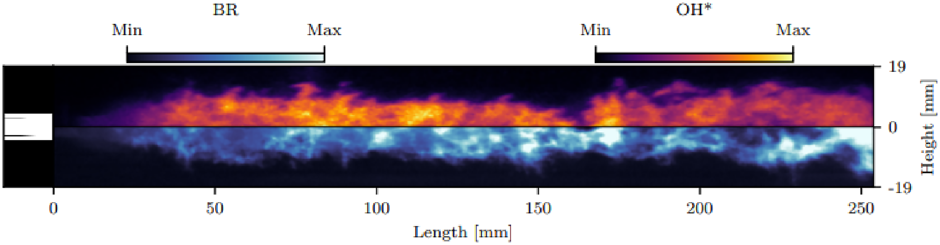
Image of a liquid oxygen-methane flame from experimental combustor Brenkammer N (‘BKN’). 47
In summary, great advances have been made in low-order acoustic modelling of complex flows. Nevertheless, the modelling of 3D modes (tangential and radial) is still an open problem. Furthermore, only the model by Schaefer et al. is capable of considering arbitrary gradients and area variations simultaneously. Lastly, none of the mentioned models can combine these effects with a distributed flame response throughout the entire chamber. Consequently, the need of new developments for rocket engine thermoacoustic simulation is clear.
Flame response modelling
The most common approaches to implement the flame response are flame transfer functions (FTFs), which are created from experimental data, and analytical models, which require an expression for the unsteady heat release. The most widely used unsteady heat release model is Crocco’s simple time lag model. 38 There are other models, such as the ones by Polifke 39 with dual time delay models and distributed time delay models, as well as frequency dependent time delays. The report published by Casiano 40 summarizes multiple time lag models.
The time lag models need to be combined with a flame model. Examples valid for laminar premixed flames include the work by Polifke,39,41 as well as from the OSCILLOS team.
32
These models are used to represent conical and wedge flames. Another work by Polifke et al.
42
slightly modifies the model based on the Rankine-Hugoniot equations and simple time lag model by introducing losses in the flame element. It introduces the pressure losses as a freely adjustable coefficient and names the model ‘
Experimentally measured FTF can also be included in the network models, as shown by Schuermans et al. 43 This approach has become very common for gas turbine combustor modelling. A common approach to obtain the FTF is the multi-microphone method. 44
In rocket engines, the measurement of time lags and gains is much more difficult than in gas turbine combustors. The work by Martin et al. 45 managed to obtain the time lag values for a sub-scale combustor, thanks to its large optical access. Obtaining an accurate experimental FTF for a rocket engine is yet to be achieved.
Limitations of existing network model elements for rocket combustion chambers
In the combustion chamber of a rocket engine, the gradients in the mean flow variables are significant. This is especially so for the speed of sound and density, which are key variables for acoustic analysis. Furthermore, these gradients extend throughout a significant length of the chamber, not allowing to consider them as discontinuities, contrary to the usual approach for gas turbine combustors. Moreover, the rocket engine nozzle also presents these strong gradients in mean flow along with a significant variation in area. Most importantly, tangential and radial modes are of high relevance for rocket engines, as they have been the cause of instability in the past. 46 As stated before, this generated a need to develop a set of new acoustic elements.
In gas turbine combustors, the compact flame assumption allows to model the entire flow as isentropic, with an entropy discontinuity at the flame. For rocket engines, due to slower atomization, evaporation and mixing, the flame length is of the order of the combustion chamber length (see Figure 1). This invalidates the compact flame assumption. Consequently, the entire flow-field needs to be solved as non-isentropic. This motivated the development of a distributed flame element which allows the spatial extent of the flame to be captured, as well as the previously described gradients in mean flow.
Novel models
In this section, the novel elements developed will be presented, showing their mathematical description and highlighting some key aspects. The full derivation for all the presented models is present in the Appendix.
One-dimensional (1D)-chamber with varying background mean flow and area
In this model, all the background flow variables are considered to be a known function of the axial coordinate. Both the background and acoustic flows are isentropic. The model allows for the computation of the longitudinal resonant frequencies of the system. The acoustic pressure and velocity are described as follows:


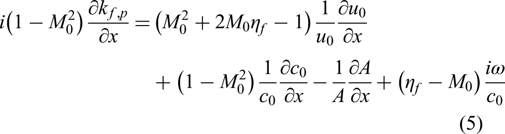
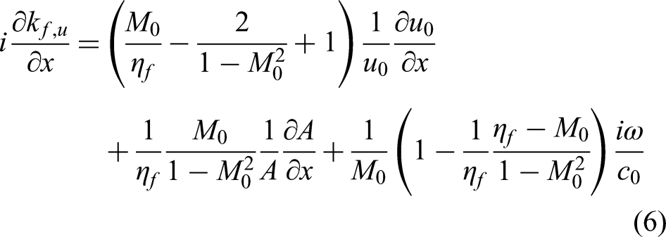
The equations for

The function
Sonic boundary condition
The expression for a sonic BC at the throat of a rocket engine (convergent to divergent transition) is:
Its derivation is present in the Appendix (equation (88)). The BC is meant to be used in this shape for the 1D isentropic element. Nevertheless, for a qualitative feel of what the BC represents, the acoustic pressure and velocity will be substituted by
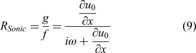
Note that for low frequencies, this approximate reflection factor equals 1 (closed BC) and for very high frequencies it approximates 0 (non-reflecting BC), which matches experimental measurements.31,48 Keep in mind that this reflection factor is only qualitative, as it has been shown that for this model the expression for the acoustic velocity carries a correction factor for the
The sonic BC for an acoustic 3D non-isentropic flow is shown next. To obtain the 3D isentropic BC it is sufficient to substitute
3D element with varying background mean flow to model transverse acoustic modes
This model considers a known, purely axial background flow and a 3D acoustic flow. Both are considered isentropic. Cross-section area needs to remain constant. The model allows for the computation of the longitudinal, radial and tangential resonant frequencies of the system. The acoustic variables are described as follows:
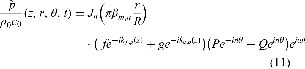
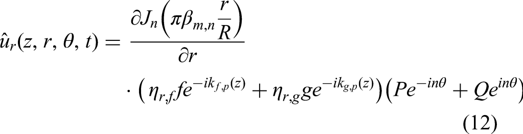
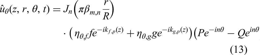
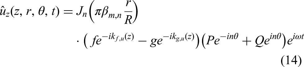
The equations for
Distributed flame response model
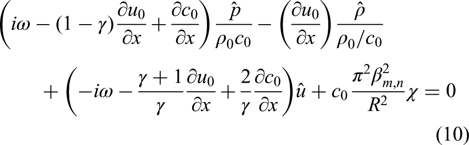
The background flow is assumed to be purely axial but not isentropic, as there is a heat release along the length of the element function of the axial coordinate. The model allows to compute the resonant frequencies of the system, along with its stability. The acoustic pressure and velocity are described as shown for the 1D isentropic element in equations (3) and (4). For the distributed flame model, the acoustic density needs an additional description as follows:
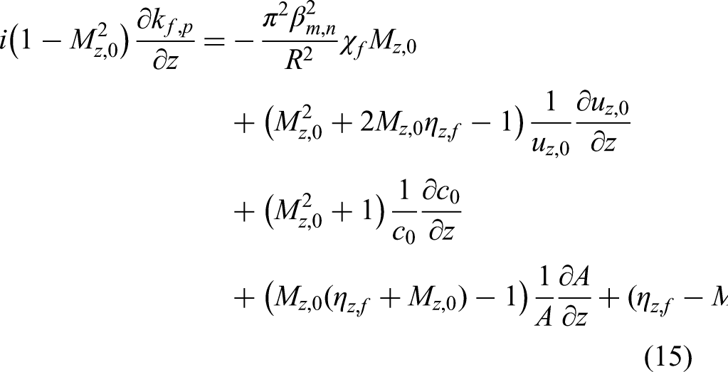
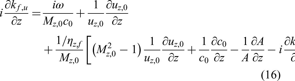
The wave numbers for pressure, velocity, and density need to be solved for, leading to a system of six uncoupled first-order ODE:
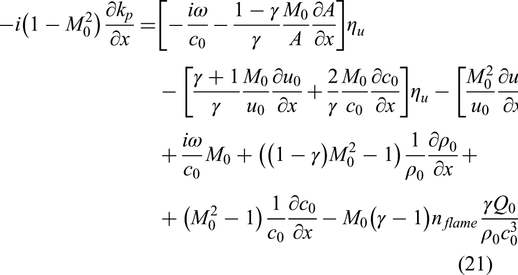
Once more, the equations for the
For the results that will be subsequently presented, the unsteady heat release was modelled as follows:
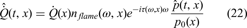
Furthermore, in this work, due to the limited experimental data available, both
Verification of models
Multiple verification steps were taken for the first model. First, the expressions for the acoustic variables are a solution of the acoustic equations, as they have been derived fully analytically. Furthermore, if the gradients of area and background flow are removed from the isentropic elements, the solutions for the 1D and 3D incompressible ducts are retrieved, respectively, (see the Appendix, equations (42) and (43)). This shows that the new model correctly describes incompressible flows.
Further verification was performed using cases with moderate gradients in background flow and/or area. The new models require only one element to describe this behaviour. They were compared with network models made of multiple basic elements from literature. One of these verification cases is highlighted next.
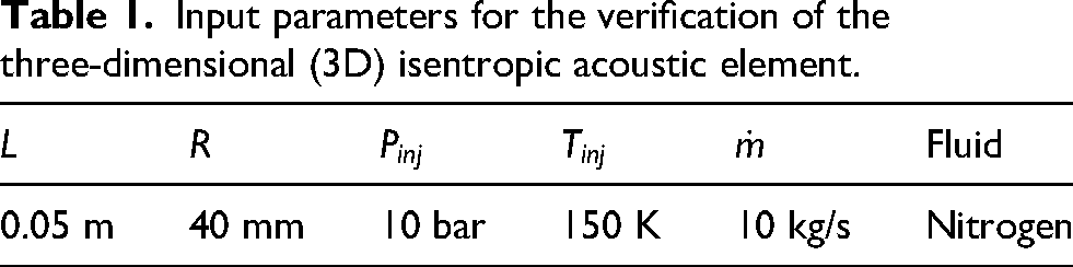
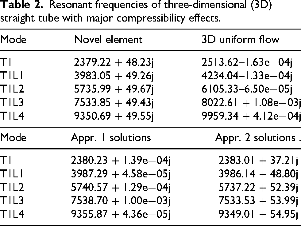
The results of the novel 3D element are compared to the results of the literature 3D incompressible tube, those of simulating the system discretized into 100 3D uniform flow elements (approximation 1) and those of the same discretization but with added compact discontinuity elements between the 3D uniform flow tubes (approximation 2). Input parameters are summarized in Table 1. The results are shown in Table 2. Given its simplicity, it was to be expected that the single 3D uniform flow element would differ the most from the novel element. Furthermore, approximations 1 and 2 both match very closely the real part of the solution from the novel element, but only approximation 2 shows a similar behaviour of the imaginary component (to be expected given that approximation 1 only contains elements that conserve acoustic energy). This shows that the new model adequately describes resonant frequency and damping rate for moderate gradients. Note that, for the more extreme gradients present in a rocket engine and especially regarding the flame, the approximations made from the basic elements get worse, which is why the new elements are needed. Their performance in more complex systems will be shown in the Results section.
Input parameters for the verification of the three-dimensional (3D) isentropic acoustic element.
Resonant frequencies of three-dimensional (3D) straight tube with major compressibility effects.
A more extreme example was also tested, where two tubes connected through an area discontinuity are considered. Both have a length of 0.05 m, left tube with area
Modelling of a compact discontinuity between two straight tubes with the newly introduced one-dimensional (1D) isentropic element.
Modelling of a compact discontinuity between two straight tubes. Solution obtained with the state-of-the-art network element for a compact area discontinuity superimposed with that of the newly introduced one-dimensional (1D) isentropic model.
Consequently, the new models have been shown to converge to the incompressible and compact solutions (no gradients and ‘infinite’ gradient, respectively), as well as always being solutions to the acoustic equations. This justifies going further into validation against experimental data.
Computational framework
The software LORESA was developed at DLR, in which these new models were implemented. Said software was used to obtain the validation results. The software is not publicly available, but a complete description of the models is present in the Appendix.
The solution procedure is simple: once the desired model is chosen, it can be computed for a given frequency. Only for the resonant frequencies of the system will the longitudinal downstream BC be satisfied. Therefore, using a minimization algorithm the set of frequencies that satisfy said BC can be found. Other approaches, such as a sweep of values of the frequency are also valid, although might be more computationally demanding.
In order to perform the computation for a given frequency, the ODE of the given model need to be integrated. This can be done with any stiff ODE solver library. It is recommended to use a stiff or adaptive solver, as the gradients in the background flow of a rocket engine can be quite large.
Running the non-optimized Python code on a single thread on a regular desktop, the average computation time required to compute the longitudinal resonant frequencies of the system are of 15 minutes for the isentropic models and around 20 minutes for the flame model. To compute the main longitudinal, tangential and radial resonant frequencies with the 3D flame model, the expected time is around 1 hour.
Experimental test cases
The described modelling environment was benchmarked with two published rocket combustor experiments of different scale and propellant combinations (liquid oxygen and hydrogen (LOX/H2) and liquid oxygen and natural gas/methane (LOX/NG)). Both combustion chambers showed operating conditions with stable combustion and unstable combustion.
Further information on the first combustor, Brennkammer D (BKD), can be found by Armbruster et al., 46 Gröning et al., 49 Armbruster et al., 50 Gröning et al. 51 and Armbruster et al.52,53 and previous studies about its stability behaviour include4,9–12,15,54–57
For the second combustor, Brenkammer N (BKN), information can be found by Martin et al.45,58,59
Results
In this section, the results obtained for two load points of the BKD engine and four load points of the BKN engine, computed using the new models implemented in the software ‘LORESA’ (Low-Order Rocket Engine Stability Analysis), are shown. In both cases, the results of the purely acoustic simulation (isentropic models) obtained with LORESA are presented first, followed by the stability analysis performed with LORESA using the novel distributed flame elements.
BKD
The background flow data for the following simulations of BKD was obtained from the work performed by Schulze. 11 The system is modelled using a single new isentropic element with an ideal closed BC at the inlet of the combustion chamber and the novel sonic BC at the throat of the nozzle.
Chamber acoustics
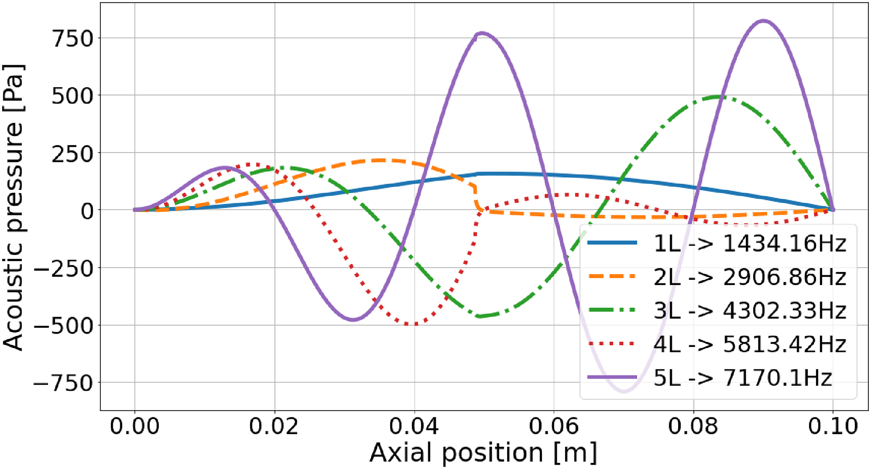
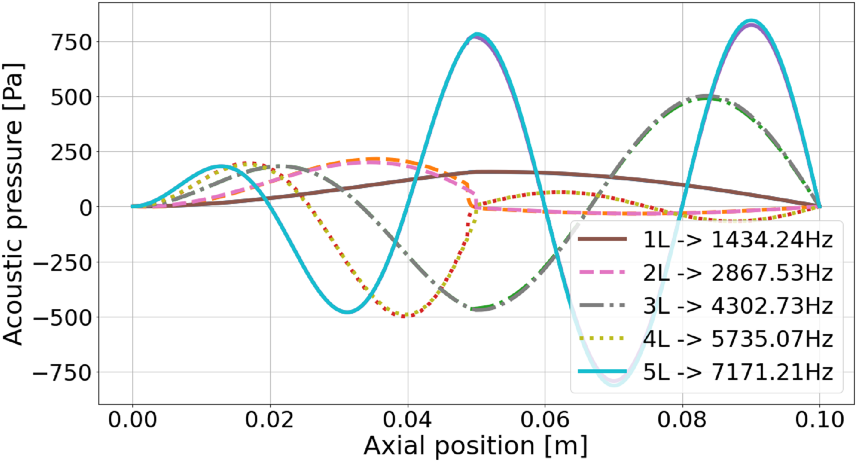
The values of the acoustic resonant frequencies computed with LORESA are compared to the experimental values obtained at DLR. The data for the so-called LP4 is shown in Table 3 and for LP3 in Table 4, respectively. The absolute error in the resonant frequencies obtained is between 0.29% and 5.18% and the mean error is 3.30%.
Resonant frequency comparison between experimental and acoustic simulations for BKD LP4.
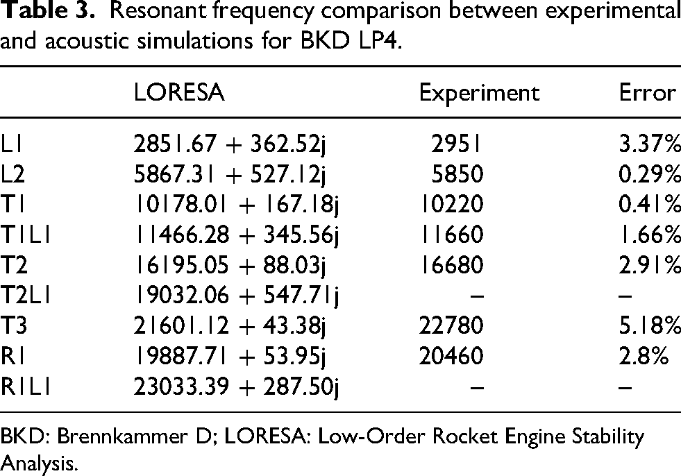
BKD: Brennkammer D; LORESA: Low-Order Rocket Engine Stability Analysis.
Resonant frequency comparison between experimental and acoustic simulations for BKD LP3.
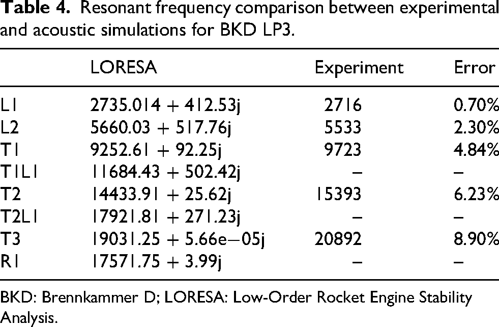
BKD: Brennkammer D; LORESA: Low-Order Rocket Engine Stability Analysis.
It is noted that LP3 presents slightly higher errors and that higher frequencies are typically predicted worse than low frequencies. It is also notable that the imaginary part representing the damping rate (negative growth rate) is positive for all the simulated frequencies. This is to be expected as the acoustic effect of the flame is not considered and, therefore, there are no excitation mechanisms.
Chamber stability
The stability of the chamber is studied using the newly developed distributed flame elements. The acoustic response of the flame is included, as well as its effect on the mean flow. The values of the boundary conditions are kept the same: closed at the inlet and the new sonic condition at the nozzle’s throat.
Given that for both load points of BKD no experimentally-measured gain nor time lag were available, a sweep of possible values was first performed. Using said sweep, a set of ‘stability maps’ was generated, for which the stable and unstable combinations of gain and time lag were identified. In Figures 4 and 5, the stability maps for the T1 and R1 modes, respectively, of LP4 are presented and in Figures 6 and 7, for LP3. The white region represents the stable combinations, the rest of the regions represent the unstable configurations, with darker colours indicating a larger number of unstable modes appearing in the simulation.
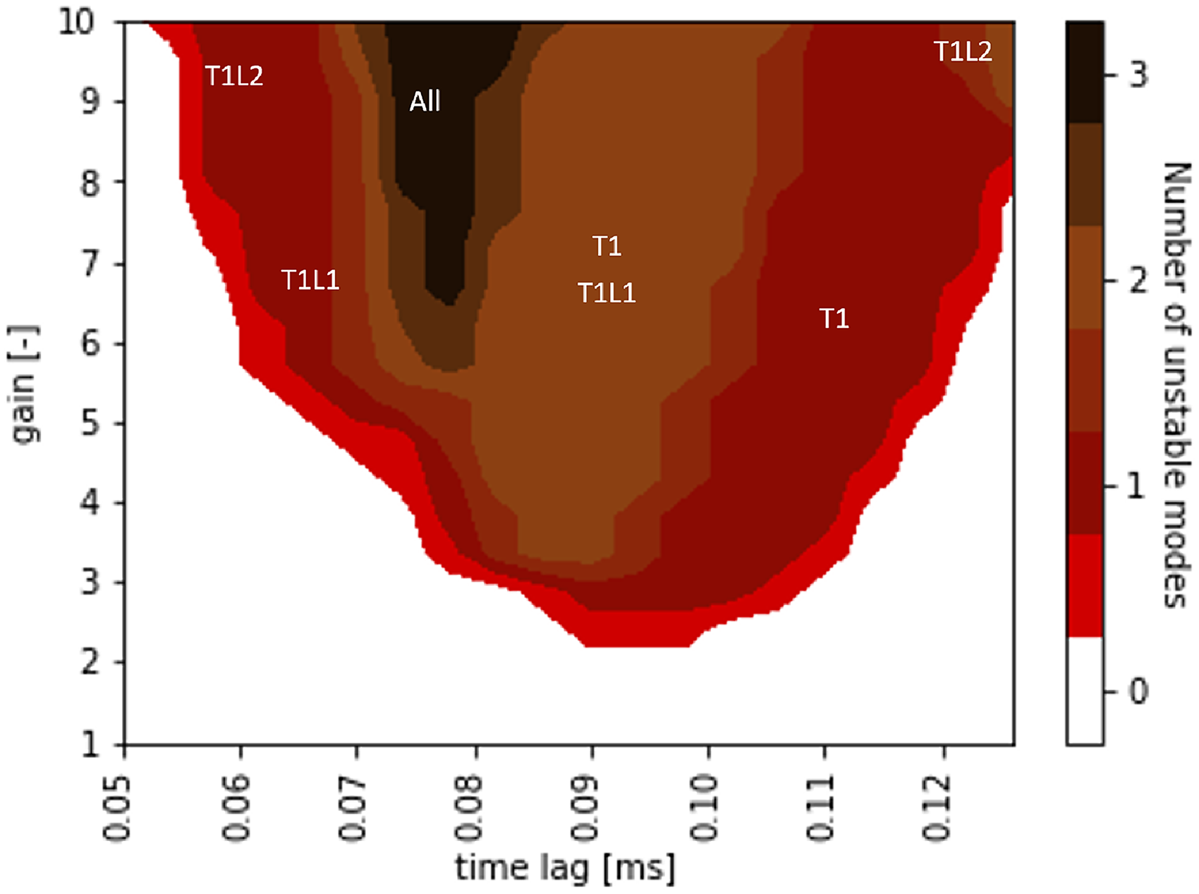
Stability map of Brennkammer D (BKD) LP4 T1Lx modes.
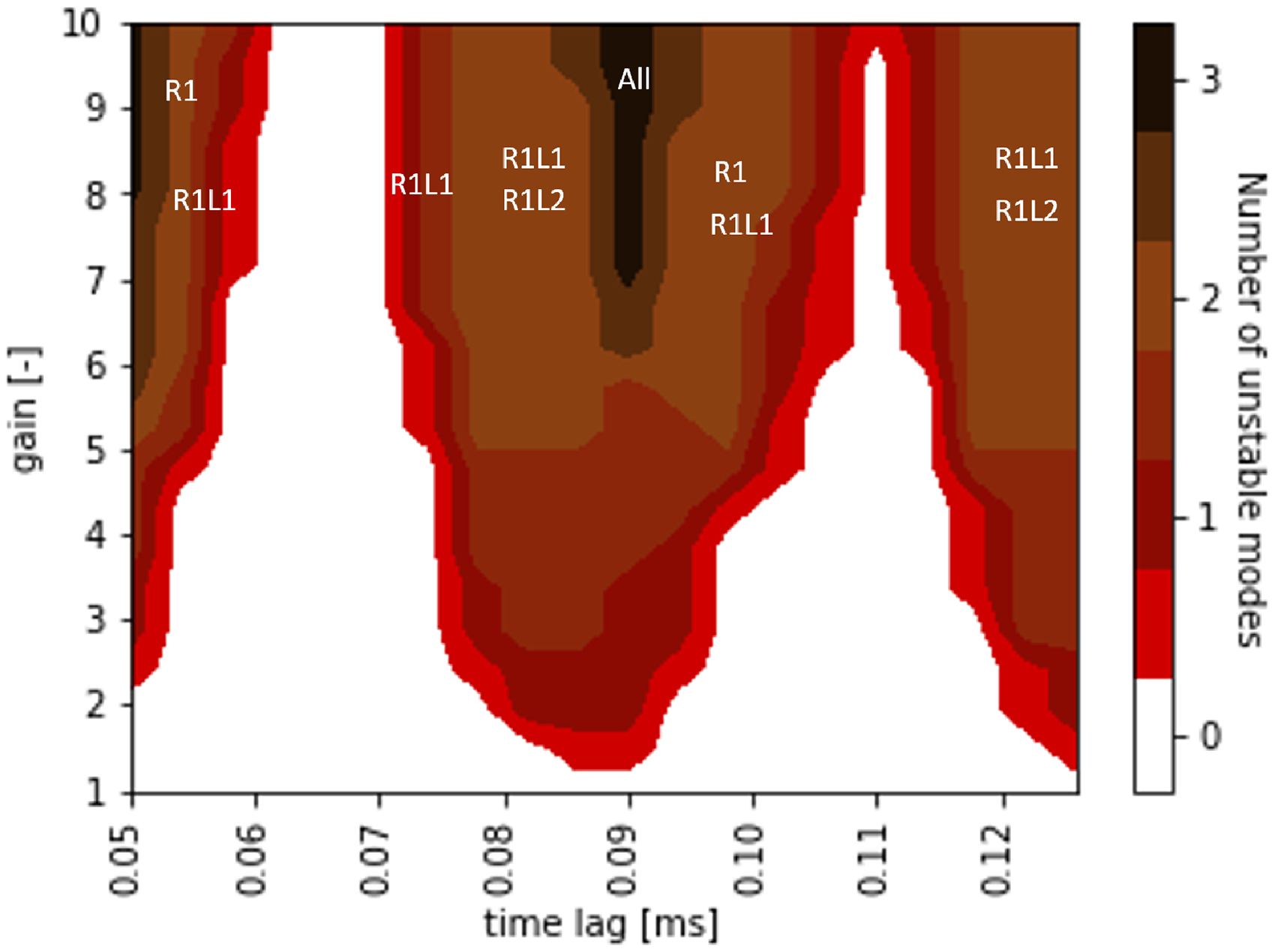
Stability map of Brennkammer D (BKD) LP4 R1Lx modes.
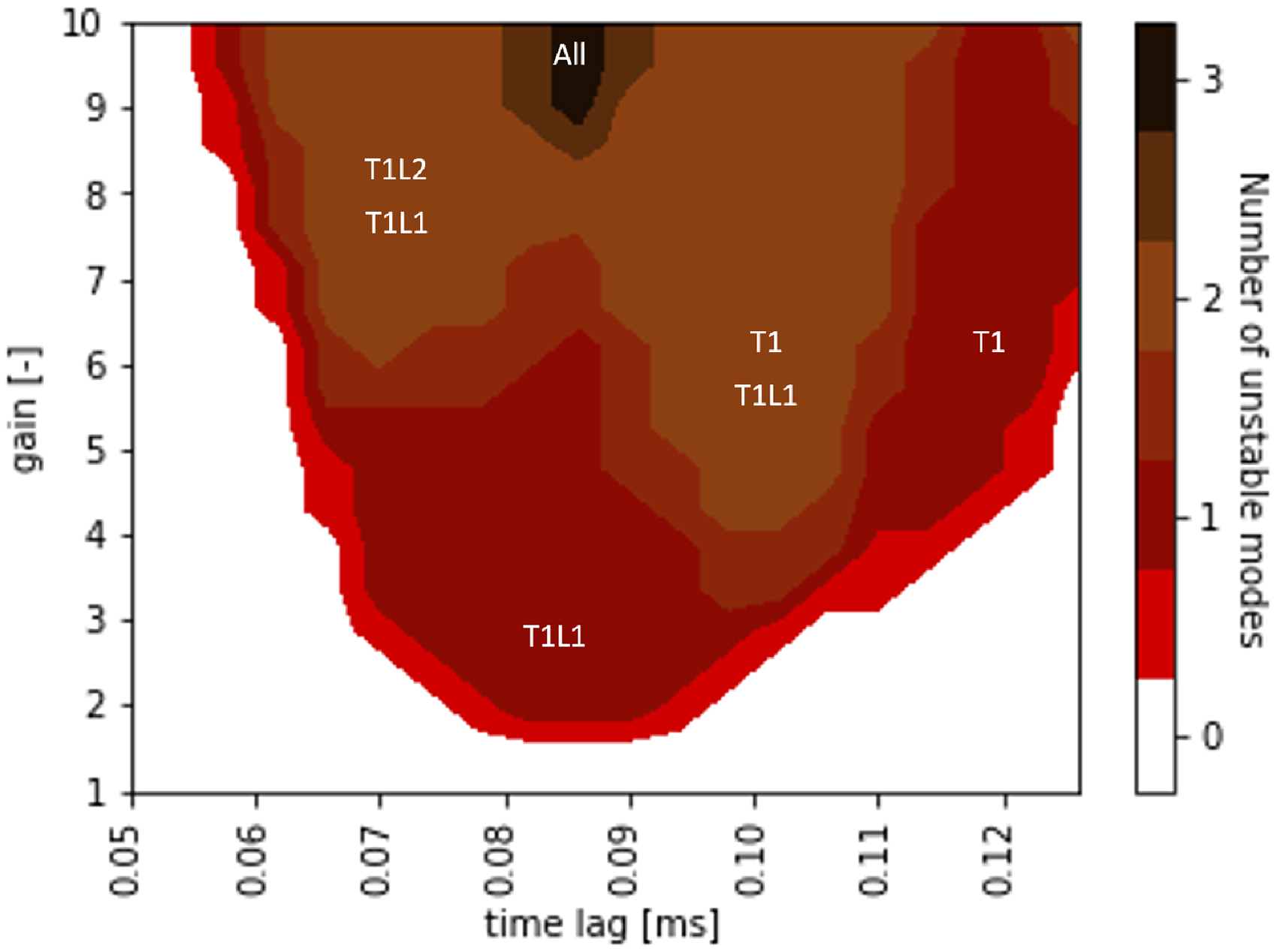
Stability map of Brennkammer D (BKD) LP3 T1Lx modes.
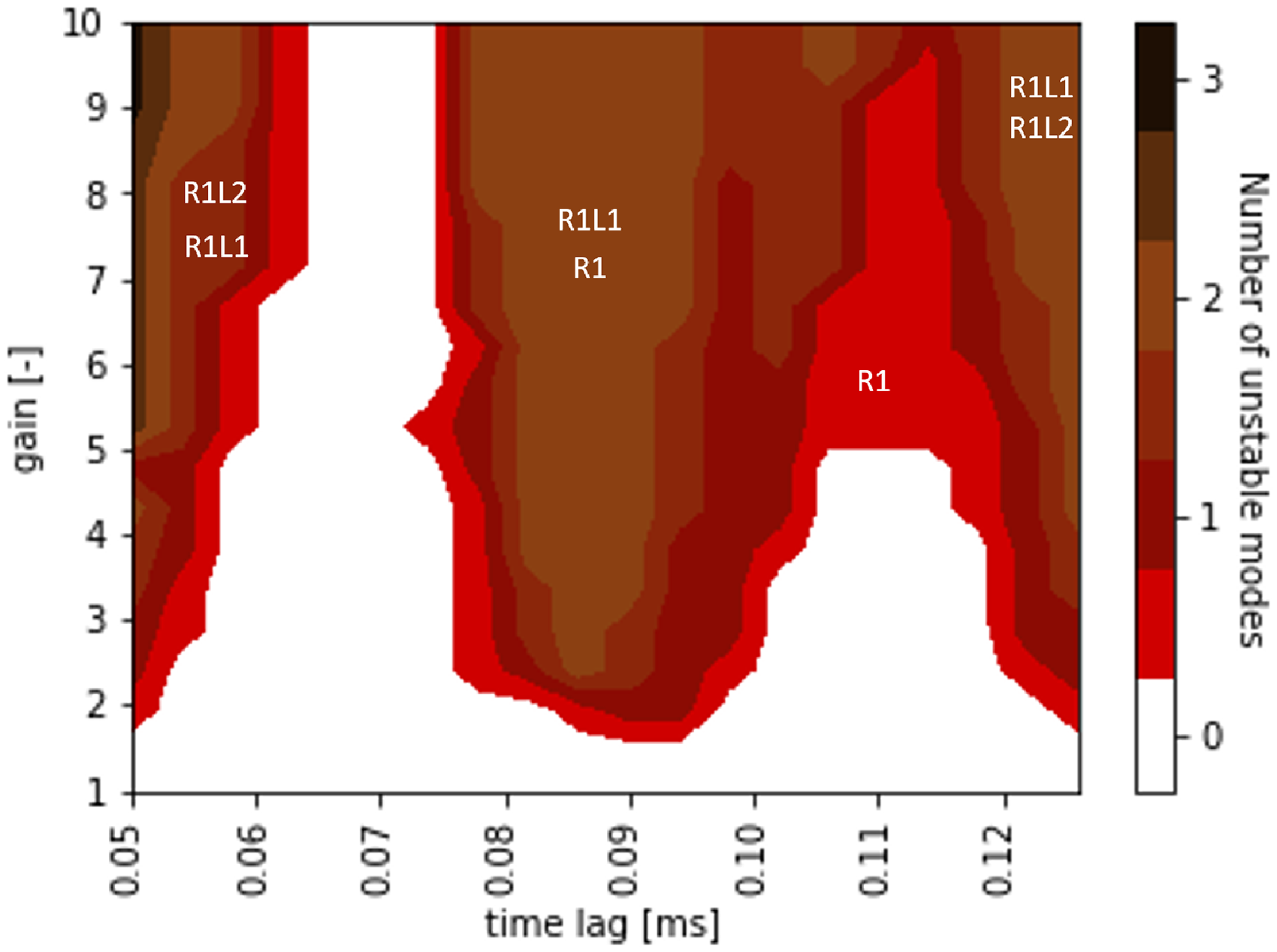
Stability map of Brennkammer D (BKD) LP3 R1Lx modes.
It is observed that the stability maps for both load points show instability for given time lags even at low gains, while for other time lag values, the system is stable even for very large gains. This can be easily related to the Rayleigh criterion. For some time, lags there is a strong coupling between the heat release and acoustic pressure, leading to instability even if the gain is low. On the other hand, other time lags are completely off-phase with the acoustic pressure, leading to stable configurations even for large gains.
For LP4, the experiment showed instability in the T1 mode. From experiment, it was found out that the R1 mode is also excited, but its amplitude is much less than the T1 mode. From the findings by Urbano and Selle, 55 it is known that the Rayleigh Index for the R1 mode is much smaller than that of the T1 mode. Furthermore, the T1 mode contributes significantly to the amplitude of the R1 mode. Thus, going to the stability map, we would expect to be at the limit between stable and unstable for the R1 mode (marginally unstable). Combining this with the clearly unstable T1, a gain around 3 and a time lag around 0.095 ms were estimated. Using these values resulted in a stable T1 mode for LP3 and an unstable T1 mode for LP4 (Table 5). For LP3, this gain and time lag also showed unstable T1L1 and R1L1 (Table 6). As the LP3 was stable, there might be some differences in the gain and time lag between LP3 and LP4 or some improvement to be made to the modelling. Nevertheless, the simulations correctly identified that the T1 mode was unstable for LP4 while stable for LP3.
Resonant frequency comparison between experimental and distributed flame simulations for BKD LP4.
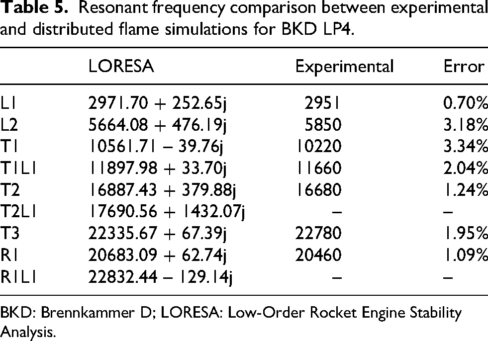
BKD: Brennkammer D; LORESA: Low-Order Rocket Engine Stability Analysis.
Resonant frequency comparison between experimental and distributed flame simulations for BKD LP3.
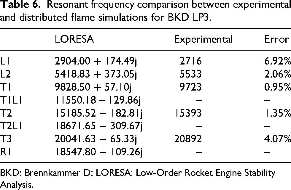
BKD: Brennkammer D; LORESA: Low-Order Rocket Engine Stability Analysis.
Using these values of gain and time lag, the resonant frequencies were computed again. The results for LP3 are presented in Table 6 and for LP4 in Table 5. The average error of the resonant frequencies is 2.41%. There is a general decrease in this error as compared to the results of the purely acoustic approach. The largest errors are now found for the lower frequencies instead of the larger ones (specially in the LP3 L1 mode). It is considered that the larger errors in the longitudinal modes, when compared to the acoustic case, could be due to a necessity to introduce a different dependence between unsteady heat release and acoustic pressure based on the mode under consideration, since tangential and longitudinal oscillations affect the combustion process differently. If this is true of longitudinal modes, it could explain why the T1L1 and R1L1 are wrongly predicted as unstable.
For both load points, experimental values for the damping rate of the T1 mode were computed by Schulze.
11
For LP3, damping was computed to be between 180 and 390 rad/s, while LORESA giving a lower value of 57 rad/s. For LP4, the damping ranges between
BKN
The background flow data for the simulations of BKN was obtained from a radial average of a 3D RANS simulation performed at DLR. As this 3D RANS simulation was performed for a different chamber configuration than the one considered in this work, the data was scaled accordingly for each load point using the chamber and flame length. The system is modelled using a single new isentropic element with an ideal closed BC at the inlet of the combustion chamber and the novel sonic BC at the throat of the nozzle.
Chamber acoustics
The values of the acoustic resonant frequencies computed with LORESA are compared to the experimental values obtained by DLR. As LP1 and LP2 have the same chamber configuration and flame length, it results in the same scaling of the background flow. In consequence, they are treated as a single simulation case and compared with both experimental cases in Table 7. The comparison for LP3 is performed in Table 8 and for LP4 in Table 9. The mean error of the BKN simulations is 2.84%.
Longitudinal acoustic resonant frequencies comparison between simulation and experiment for BKN LP1 and LP2.
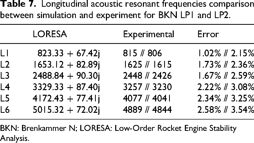
BKN: Brenkammer N; LORESA: Low-Order Rocket Engine Stability Analysis.
Longitudinal acoustic resonant frequencies comparison between simulation and experiment for BKN LP3.
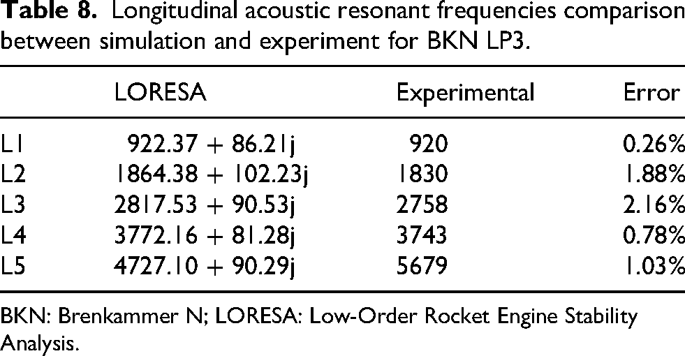
BKN: Brenkammer N; LORESA: Low-Order Rocket Engine Stability Analysis.
Longitudinal acoustic resonant frequencies comparison between simulation and experiment for BKN LP4.
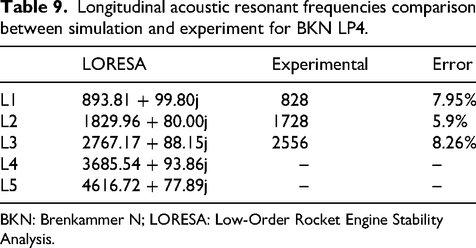
BKN: Brenkammer N; LORESA: Low-Order Rocket Engine Stability Analysis.
The results for LP4 are considerably worse than for the other cases, while LP1, 2, 3 have similar errors to BKD. It is believed that this might be caused by the background flow data scaling, as the flame length for LP4 case is unknown since it extended beyond the end of the window.
Once again, all the frequencies are predicted with positive damping rates and thus as stable since the excitation caused by the unsteady heat release is not included in this purely acoustic analysis.
Chamber stability
The stability of the chamber is studied using the newly developed distributed flame elements. The acoustic response of the flame is included, as well as its effect on the mean flow.
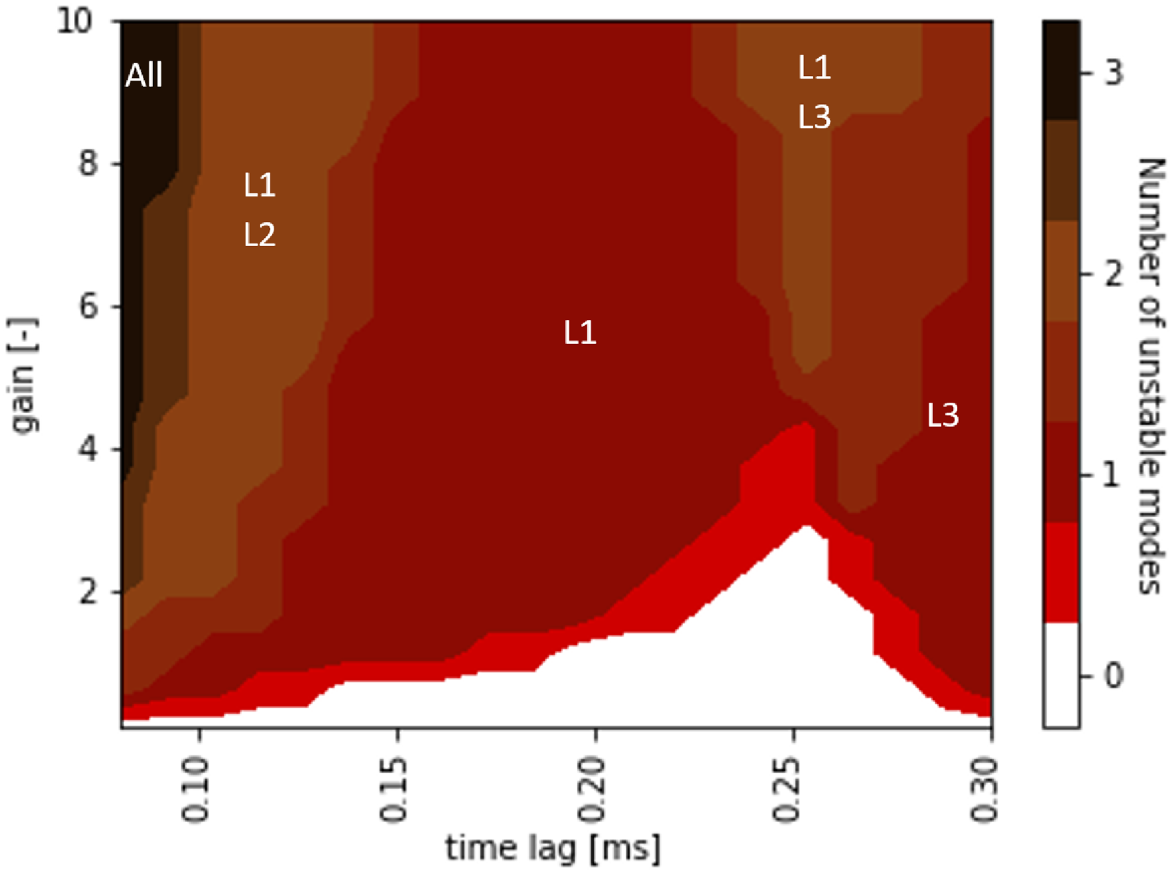
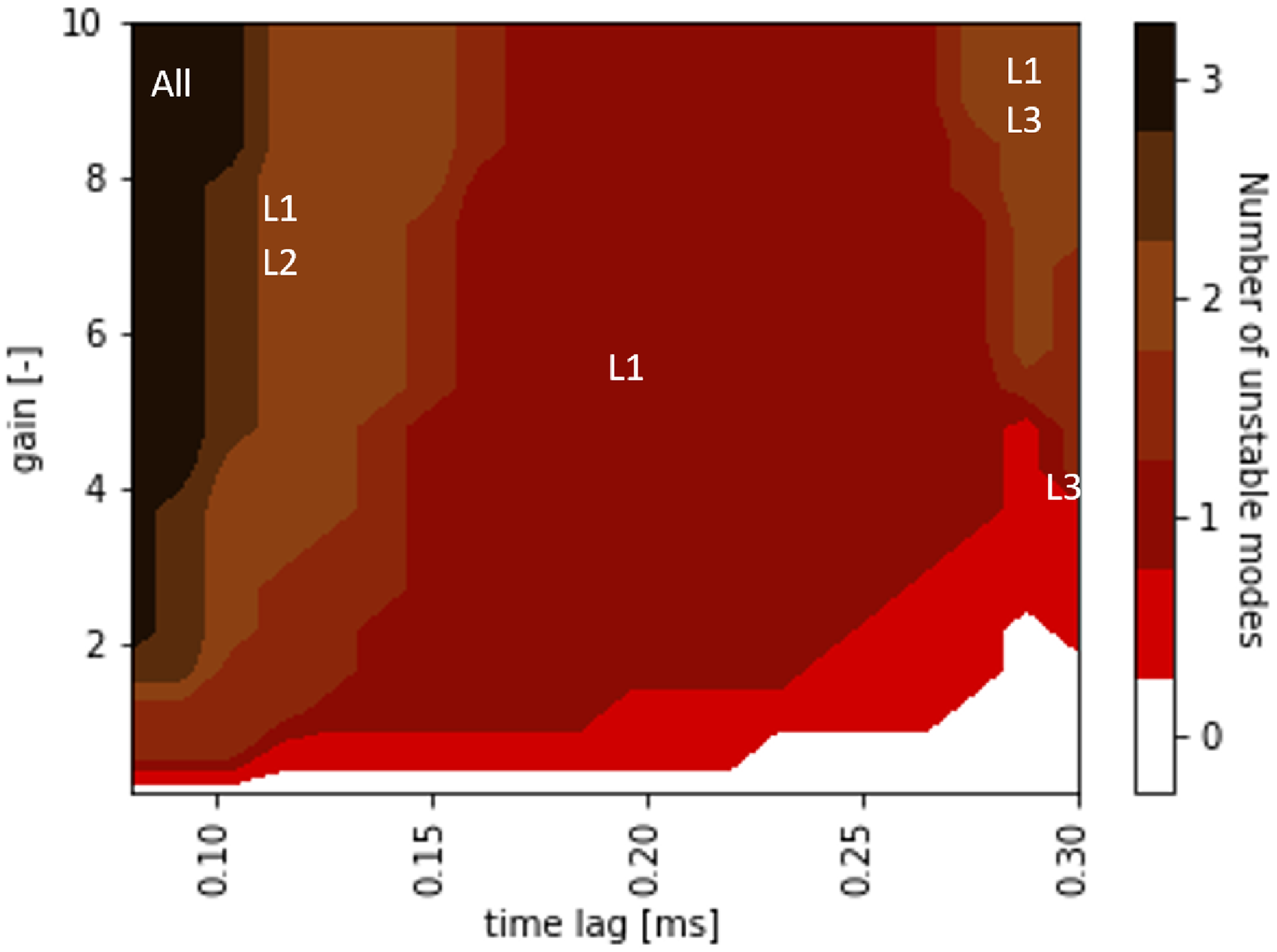
For BKN, the time lag values for all four load points were experimentally measured 60 and provided in Table 10. As the gain is still unknown, the stability maps were once again generated via a sweep of various combinations of gain and time lag values. The stability map of the longitudinal modes for the short chamber (LP1 and LP2) is presented in Figure 8 and for the long chamber (LP3 and LP4) in Figure 9. Once again, the white region represents the stable combinations, the rest of the regions represent the unstable configurations, with darker colours indicating a larger number of unstable modes appearing in the simulation.
Stability map of Brenkammer N (BKN) short chamber Lx modes.
Stability map of Brenkammer N (BKN) long chamber Lx modes.
Experimental determined time lag values for the four BKN LPs. 60
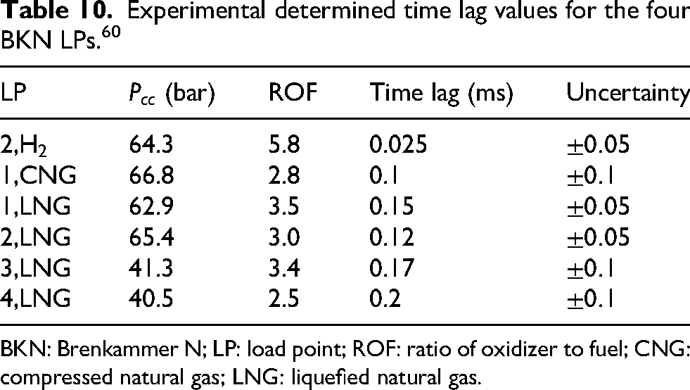
BKN: Brenkammer N; LP: load point; ROF: ratio of oxidizer to fuel; CNG: compressed natural gas; LNG: liquefied natural gas.
The first finding to be drawn, is that the lengthening of the chamber offsets the region of stability. The longer chamber (corresponding to LP3 and LP4) results in larger time lags needed for stability at high gains. As the length fundamentally changes the resonant frequency of the system, this once again shows that the code predicts coupling of the acoustic pressure and unsteady heat release based on the time lag value.
Using the stability maps and the experimentally measured values of the time lag, as well as the observed stability behaviour, an estimate of the gain can be obtained. Given that all four load points are relatively similar, a common gain value will be assumed. Since LP4 was at the boundary of stability (growth rate close to zero) and the other load points unstable, it is concluded that the gain should be close to 1. This gain results in matching stability between experiment and simulation.
Using the experimentally measured time lag values along with the gain values obtained from comparing the stability maps with the experimental observations, the four load points were once again simulated. The resonant frequencies computed using the distributed flame model are compared with their respective experimental measurements in Tables 11 to 14.
Longitudinal acoustic resonant frequencies comparison between distributed flame simulation and experiment for BKN LP1.
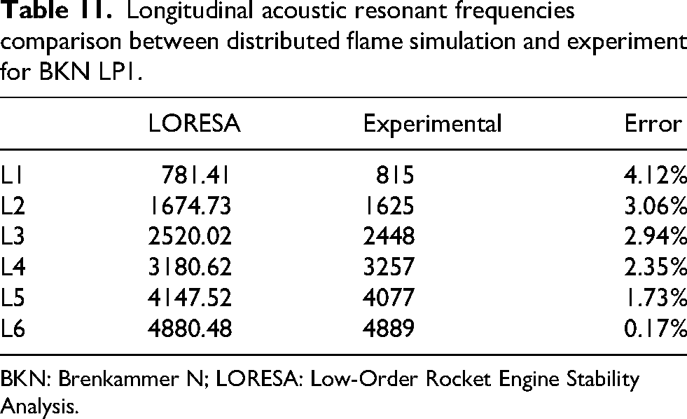
BKN: Brenkammer N; LORESA: Low-Order Rocket Engine Stability Analysis.
Longitudinal acoustic resonant frequencies comparison between distributed flame simulation and experiment for BKN LP2.
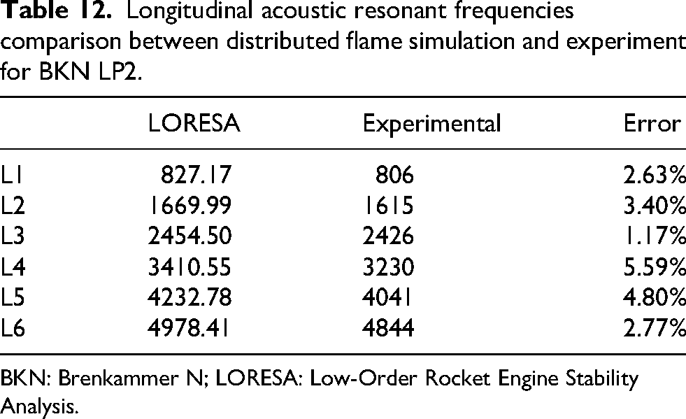
BKN: Brenkammer N; LORESA: Low-Order Rocket Engine Stability Analysis.
Longitudinal acoustic resonant frequencies comparison between distributed flame simulation and experiment for BKN LP3.
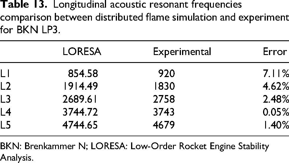
BKN: Brenkammer N; LORESA: Low-Order Rocket Engine Stability Analysis.
Longitudinal acoustic resonant frequencies comparison between distributed flame simulation and experiment for BKN LP4.
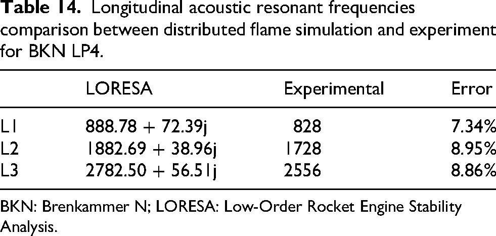
BKN: Brenkammer N; LORESA: Low-Order Rocket Engine Stability Analysis.
For the results of load points 1, 2 and 3, the imaginary part was not included. The resonant frequency was measured at the limit cycle at which, due to the longitudinal instability, there is a significant shortening of the flame. On the other hand, given the linear nature of the code, the stability prediction needs to be done at low amplitudes, while the acoustic oscillations are still small. Consequently, the flame length used for stability prediction is much larger than the one used to predict the resonant frequency of the shorter flame configuration present at the limit cycle. Note that, for the longer flame (corresponding to the linear case), modes 1, 2 and 3 are correctly predicted as unstable, as shown in the stability maps, it is just for the shorter flame (corresponding to the behaviour at the limit cycle) where the damping rates are not correctly predicted.
The average error for all BKN simulations with distributed flame is 3.78%. This error is slightly larger than the one for the acoustic analysis. This could be related to the frequency being simulated with a linear tool but being measured at the limit cycle. Additionally, the distributed flame model generally exhibits larger errors on longitudinal modes than transverse modes.
Summary and conclusions
A set of new models for acoustic network elements have been developed which allow for a more accurate description of the acoustic field in rocket engine combustion chambers compared to the models highlighted in the state-of-the-art. The new models predict the acoustic resonant frequencies of the system for both longitudinal, tangential and radial modes as well as their stability. The models were implemented in an acoustic network environment tool called ‘LORESA’. LORESA is capable of simulating both the injectors and combustion chamber including the convergent nozzle of a rocket engine.
The most notable of the new elements is the distributed flame model, which can be used to predict the stability of the longitudinal, tangential and radial modes of a rocket engine combustion chamber. The model accounts for typical characteristics of cryogenic rocket combustion chambers, such as a long flame, non-isentropic behaviour and strong axial gradients in speed of sound and density.
The average error in the prediction of resonant frequencies obtained with the acoustic model was 3.4%. The errors for the predictions of the distributed flame model had an average of 3.56%. The stability of the main modes was correctly predicted for all the validation cases. The average error for the flame model was slightly higher than for the acoustic modelling. Nevertheless, for the cases in which most of the resonant frequencies were measured in the linear regime (BKD), the results proved to be much better for the stability modelling than for the purely acoustic modelling.
In conclusion, the newly developed models are able to give a stability prediction both for LOX/H2 and LOX/NG. The model also correctly differentiates the stability behaviour of two load points based on differences of inlet conditions or chamber length. The prediction of thermoacoustic resonant frequencies is achieved with low errors even across the different propellants and geometries tested. The linear stability analysis of the benchmarking test cases was successful, identifying values of gain and time lag that gave a correct stability behaviour across the different load points for each combustion chamber, matching their experimental behaviour.
Footnotes
Ethical considerations
No ethical approval was required.
Author contributions
WA: conceptualization; JH: resources; WA, JM and MB: data curation; NJC: software; NJC: formal analysis; WA and BZ: supervision; NJC and WA: investigation; NJC and WA: validation; NJC, WA and JM: original draft preparation; NJC, WA, JH and MB: review and editing; NJC and WA: visualization; WA, NJC, BZ and JH: project administration; JH: funding acquisition.
Funding
The authors received no external financial support for the research, authorship, and/or publication of this article.
Declaration of conflicting interest
The authors declared no potential conflicts of interest with respect to the research, authorship, and/or publication of this article
Data availability statement
The original contributions presented in this study are included in the article. Further inquiries can be directed to the corresponding authors.