
Abstract
The global COVID-19 outbreak made our society aware of the significant role that mask-wearing plays in the prevention of viral transmission. Almost everywhere, world health authorities have been recommending the use of face masks in public spaces, with some even making it mandatory. Therefore, a significant rush is underway to develop automated face mask detection systems for surveillance purposes in areas such as transportation systems, shopping malls, and educational institutions, with the aim of monitoring the implementation of face mask policies. This work introduces a unique approach to enhance face mask detection by combining an Active Learning (AL) system with a Convolutional Neural Network (CNN), and fine-tuning the CNN's hyperparameters using a Genetic Algorithm (GA). We use the AL framework to query the most informative data samples, which not only minimizes the labelling cost but also achieves high model accuracy. To improve CNN's performance, hyperparameter optimization uses a genetic algorithm to optimally select the network parameters. The study leverages transfer learning and pruning on the CNN model to improve results. Pruning simplifies the network for faster inference, while transfer learning increases accuracy by leveraging the weights and biases of previously trained models. Benchmark datasets assess the proposed method, demonstrating its superior performance in face mask detection with higher accuracy and robustness compared to previous methods. According to the experiment, there are different levels of accuracy in training different active learning sampling strategies that use the transfer of learnt CNN pruned. The entropy sampling method outperforms all other methods, achieving an accuracy of 98%. We compared the transfer-learned pruned CNN model with the Corona mask two-stage CNN model and the fine-tuned Yolov6 model for real-time face mask recognition.
Keywords
Introduction
The COVID-19 pandemic has been a tragic reminder for all of us of the pivotal role, played by face masks in the fight against the spreading virus. 1 Mask-wearing became a global priority when public health authorities rushed to state that it is one of the crucial preventive measures against the transmission of SARS-CoV-2 virus. 2 The requirement and recommendations for the use of face masks became normal in public spaces. It became a crucial aspect of the public health movement focused on the decrease of viral infection transmission. However, the implementation of face masks has exposed a new requirement for efficient monitoring mechanisms to assure compliance. 3
Active learning, a type of algorithm that is designed to choose the most informative samples for the training dataset, is very efficient in the process of data annotation for image classification tasks. 4 The overview of the active learning is presented in Figure 1. This iterative process includes the algorithm choosing data points that it considers to be the best for the model's improvement, thus, cutting down the manual annotation of large datasets. 5 Through the intelligent selection of the samples that are to be labeled, active learning algorithms can greatly decrease the annotation work that is needed while at the same time, still maintaining high classification accuracy. The selected active learning techniques in this study are entropy sampling, 6 least confidence sampling, 7 random sampling, 8 margin sampling, 9 and k-means sampling, 10 which are used to choose the most informative data points for labeling in the task of face mask detection using deep convolutional neural networks. These techniques make the model concentrate on the samples that are the most uncertain or ambiguous, thus the training process becomes more efficient and effective.
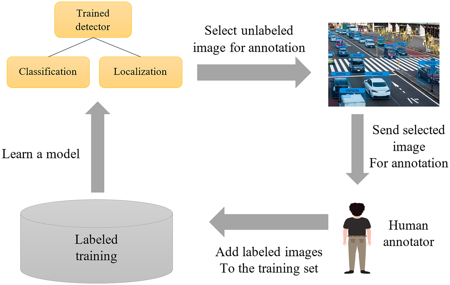
Overview of active learning flow.
In the middle of the world's first-ever public health emergency arising from the coronavirus, the urgent need to develop and implement a system of reliable and efficient control over mask compliance has become the head of the global agenda. 11 The effectiveness of the mask-wearing policy is directly proportional to not only its wide implementation, but it equally depends on the sophistication of the enforcement and monitoring mechanisms in place for compliance. However, usual methods of control compliance, such as manual observation or sporadic spot-checks have their limits. 12 They are manpower intensive, need massive personnel and time, and have room for errors that are embedded in human judgments. Besides, the traditional approaches often come short at the level of solving the whole problem and treating its complexity. 13 During this pandemic, the demand for practical and scalable solutions is more than ever needed to overcome the existing limitations and make sure the mask-wearing rules are properly applied in various places.
Traditional compliance methods for monitoring face mask usage include manual inspections by security personnel in public spaces, such as transportation systems, shopping malls, and educational institutions. 14 These methods are labour-intensive and time-consuming, relying on human oversight to ensure adherence to mask-wearing policies. Basic surveillance camera systems are used for visual monitoring, but they often lack advanced mask detection capabilities. Public announcements, signage, and manual reporting mechanisms also play roles in encouraging compliance. Temperature scanning stations and manual spot checks are employed to enforce mask-wearing. 15 While these methods can be effective, they are often inefficient and prone to human error, underscoring the need for automated solutions like the proposed deep-learning-based face mask detection system using CNNs and active learning techniques.
Nevertheless, this study will be discussing more profoundly than just the accuracy that includes active learning - a purposeful method that is aimed at streamlining the model and making it more efficient and effective. The concept of active learning implies a purposeful method of data annotation that aims at optimizing the labeling process through the selection of the most informative data instances for annotation. This methodology also maximizes the information gained from the selected data samples and thus minimizes the annotation effort required for model training which is one of the most expensive failures in the data-limited domain. Time is of the essence since the world is on the verge of breaking the chain of COVID-19 transmission at present, thus mask-wearing compliance monitoring is a significant step towards reducing the spread rate. 16
To meet this demand, the research utilizes the socialites of deep learning, active learning, and creative optimization methods to put forward a new face mask identification method. Extensive learning through the use of CNNs is included as a core component of the proposed strategy. CNNs are, indeed, the best in their class when it comes to image classification tasks which makes them the perfect fit for the complex face mask detection work. They can differentiate and recognize the unique characteristics of people wearing masks by their capacity to detect complex features and patterns from visual data. The research notes that although accuracy may be high, it may not solve the face mask detection vulnerabilities completely. Therefore, it does it by deploying AL—the right methodology that is focused on improving annotation and making the best use of the scarce labeled data. Smartly picking the most informative data points for annotation, active learning reduces the interval of annotation needed for model training and at the same time enhances the model's efficacy and responsiveness for different scenarios.
The objective of this study is to create a powerful and precise face mask detection system that is successfully deployed into the existing framework, to improve public health and safety measures. The major contributions of this study are as follows:
The study uses active learning, a method in which the model picks the most informative unlabeled data points for labeling, thus, the labeling effort and the training efficiency are reduced. To put it differently, it is a pool-based sampling scenario where a pool of data is assumed to have only a small fraction labeled, and five sampling techniques including entropy sampling, least confidence sampling, random sampling, margin sampling, and k-means sampling are used to select data points for labeling. The selection of the samples for labeling is based on the model's uncertainty in its predictions, which gives priority to the most uncertain samples. The process starts with the selection of samples from the unlabeled pool, which serves as a benchmark for the comparison with other active learning techniques. An optimization algorithm, GA is employed to tune the hyperparameters of the CNN, effectively optimizing network configuration to achieve superior performance in face mask detection tasks. This study utilized Transfer learning to enhance CNN performance by transferring knowledge from pre-trained models, while pruning simplifies the network structure for faster inference without compromising accuracy. The proposed method is rigorously evaluated on benchmark datasets, demonstrating significant improvements in accuracy and robustness compared to traditional methods and state-of-the-art models like the Corona mask two-stage CNN and Yolov6.
The rest of the paper is organized as follows: A literature review survey including existing research, motivating the proposed framework is presented in section 2. A detailed description of the proposed approach is presented in Section 3. Simulation results showcase the framework's performance, followed by a discussion on implications and limitations in section 4 and section 5 respectively. Section 6 presents the conclusion discusses findings and future research directions.
The research study of the team Habib 17 was trying to create an accurate and time-efficient deep learning-based model for real-time face mask detection. The process was composed of a comprehensive examination of the different deep learning architectures. Out of all these, the researchers chose MobileNetV2 as the backbone. They developed their model in that the autoencoder to perform abstract representations as well as augment the data was broadly applied. The study underlined the essence nature of immediate face mask recognition in the prevention of COVID-19 transmission. Their model with an accuracy rate of state-of-the-art models is the manifestation of a long and exhausting development process through an experiment on every aspect of the model. The research project gave me a chance to evaluate real-time face mask detection. The authors, Ilyas and Ahmad 18 designed a powerful deep learning model enhanced for automatic face mask detection. They employed the deep learning algorithm by feeding a lightweight model and deploying different classifiers for face mask detection with MobileNetV2 acting as a feature extractor. The cameras placed in public places helped them to collect data that they, in turn, made use of to achieve excellent performance on larger sets of data and showed the model's capacity to operate in real-time. Nevertheless, the study pinpointed the limitations such as user inspection and the lack of feather-light models.
Malakar, Kumar, and Majumdar 19 concentrated on using a real-time face mask detection method built on CNN and OpenCV. The team used a two-layer CNN model trained on 12,000 images which showed not only high-test scores but also no overfitting. Although the work established the effectiveness of real-time mask detection, they highlighted the product's limitations, including only using one technology and dataset, as well as no discussion on how it would be used in the real world. The topic of the three researchers, Sethi, Kathuria, and Kaushik, 20 was the same that was reducing the risk of coronavirus spread using the techniques of deep learning for face mask detection. Their approach was based on the combined use of an ensemble of detectors, transfer learning with ResNet50, and experimentation with the baseline models to mirror the performance to provide high precision and speedy operation. As their model was focused on developing an exceptionally accurate approach for recognizing non-masked faces in public, their proposed technique reached an accuracy of 98.2% when they used ResNet50.
In their study, De Magistris et al. 21 presented an automatic CNN-based algorithm for face mask detection, which can be particularly useful for the identification of individuals who are not wearing masks during the COVID-19 pandemic. This technique involved designing a CNN-approach model more suitable for attracting faces covered by surgical masks. After a comprehensive assessment of their model on unmasked and masked faces with the test set, which was over 96% precise in facial mask detection, the team was satisfied with the accuracy of their model. Not only did the study show the stability of the model for different mask types and fitting variations as commonly found in hospitals, but it also reached the highest accuracy and generalization rate in comparison with the existing model.
Another team, Athif and colleagues, 22 was focused on the issue of face mask detection under low light conditions. In their research, they applied the CNN method. The implementation of their methodology was via a CNN model with data transformation, processing, augmentation, and the prediction of face mask steps. Noteworthy, the model which was based on the convolutional neural network got a 98% accuracy in identifying those who wore face masks under low light conditions. Nevertheless, the research drew attention to several limitations, including not fully explaining the reasons people do not wear masks in low light conditions and the focus on recreational images recorded under low light, which limit the study's ability to generalize beyond the context of this specific situation.
In his research presented at the 2021 Integrated Communications Navigation and Surveillance Conference (ICNS), Zhang 23 introduced a real-time deep transfer learning model designed for facial mask detection. The methodology focused on developing a facial mask detection software model utilizing Deep CNN (DCNN) and integrating computer vision techniques for facial detection. Zhang has developed a system that employed deep learning models to perform binary classification of mask detection which has yielded an outstanding validation accuracy of 98%. On the other hand, this accomplishment brings an opportunity to lessen the number of human staff involved in managing mask-wearing compliance, as well as to give immediate feedback in real-time surveillance systems, thus helping with public health efforts.
Similarly, Ling et al. 24 presented a new method to identify mask-wearing in almost real-time based on deep learning. Their approach was to do it by fully utilizing human posture recognition, CNNs with Convolutional Networks, and also supervised learning for face mask detections. Cropping the imaged area to the mask region the authors from Lin et al. managed to achieve a recognition accuracy of 95% only. 8% only during the daytime while 94% is at night. In these scenarios, CO2 effluence at night will be reduced by 6%, at various times. This novel technique may have an impact on face mask detection practices, namely, in places where fast response is of importance for keeping the safety of the public and ensuring adherence to health norms.
Venugopal and others 25 proposed a cloud-based intelligent monitoring system to reduce the issue of mask violation detection by the use of alert simulation. Their approach employed deep learning techniques and convolutional neural network methodologies, which are based on cloud computing, for face mask detection. The study was summarized as the CNN classifier has shown the best results on the computer vision tasks giving a precision of 98%. Max Pooling was used to determine if the person wore a mask. Although the paper did not address limitations, some inferences can be made regarding potential constraints from discussing topics like model accuracy, real-time implementation, technological infrastructure, and mask-wearing rules, which opens up areas for further research.
Pandey and Bhaidasna 26 introduced a new model of a Deep Learning-based Face Mask Detection system with Auto-indignant. Their approach centered around essential machine learning instruments like TensorFlow, Keras, OpenCV, and Scikit-Learn for exact face and mask recognition. Through this work, they have been able to hone the parameters of the Sequential Convolutional Neural Network model and take it to the next level. How Pandey and Bhaidasna discovered that a face mask could be detected precisely through the use of very basic machine learning tools, was the result of their studies. By implementing this method, not only the positioning of faces and mask detection but also further customizing settings for quality detection are achieved. The study is noteworthy because it reveals the application conditions of the model and the significance of identification accuracy and efficiency for face mask detection systems. Moreover, such research advocates for an extensive examination of optimization options to optimize the model's effectiveness.
The summary of the literature review is presented in Table 1.
Summary of literature review with their methodology used, main findings, and limitations.
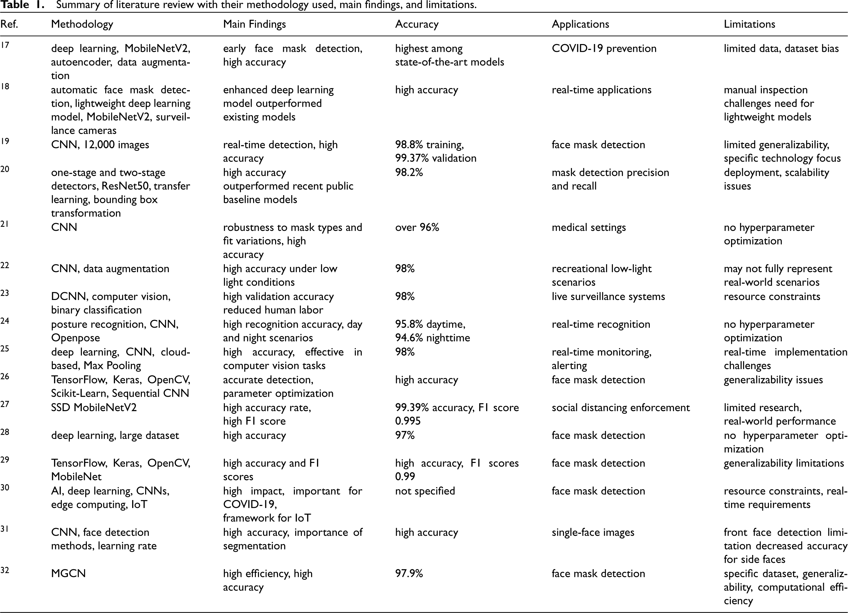
Summary of literature review with their methodology used, main findings, and limitations.
The literature review has revealed some research gaps that require further focus. The issue of models’ limited applicability for different populations, mask types, and environmental conditions is another thing to note. Many research works focus on the analysis of a single dataset or use a small variety of data sources. Such an approach may cause the model to be biased and would not perform well in real-world situations. Besides these, there has been a lack of proper evaluation of how models perform in real-world conditions which could be different lighting and varied mask-wearing habits. Another research problem is the challenge of integrating face mask detection models in real-time surveillance systems or IoT devices due to the high computational demands that they impose. Some studies try to use small-sized models, but the most complicated task is to find the optimal balance between accuracy and efficiency. Besides, the ethical and privacy issues, that real-time face mask detection in public spaces involves, especially the data collection and processing, must be considered carefully.
The study adds to the literature by presenting a CNN-based method for the detection of face masks with the help of active learning techniques. This strategy is a strong solution that is very essential for the implementation of automated systems that can track and monitor the implementation of mask-wearing policies in public areas. Active learning strategies are incorporated by the study to reduce the annotation effort that would be needed to train the model and for the optimization of the use of limited labeled data. This leads to more effective training of the model and improved performance. The study contributes to the knowledge gap in the literature by comparing the performance of active learning sampling methods like entropy sampling, margin sampling, least confidence sampling, and others for improving the accuracy of mask detection. The research evaluates the suggested transfer-learned pruned CNN model against the existing models like the Coronamask two-stage CNN model for real-time face mask recognition. The proposed model comes ahead of the alternatives in terms of training time, accuracy, precision, and recall, thus it further solidifies its worth in the field.
Materials & methods
The proposed method combines active learning with deep convolutional neural networks for the detection of face masks, targeting to reduce the data labeling effort and to achieve the best performance. In active learning, the model automatically selects the most informative unlabeled data points for labeling, thereby, achieving a better training process in terms of efficiency and effectiveness. The approach assesses various sampling techniques that apply to the pool-based sampling scenario, for example, entropy sampling, least confidence sampling, random sampling, margin sampling, and k-means sampling, to discover the best method for locating data points that will lead to the most significant improvement of the model. The proposed approach selects the most informative data points with the use of entropy sampling by its capability to choose them with high information content, especially when the model is uncertain about the labels. To get even better results, the method takes advantage of the transfer learning and pruning applied to the CNN model. Pruning will simplify the network and make deduction faster, whereas transfer learning will increase the model's accuracy by utilizing the previously trained ones’ weights and biases. To improve CNN's performance, hyperparameter optimization is conducted using a genetic algorithm to optimally select the network parameters. This blend of techniques is responsible for the fact that the system is more accurate and effective in recognizing masks in images and videos. The overview of the proposed approach is presented in Figure 2.
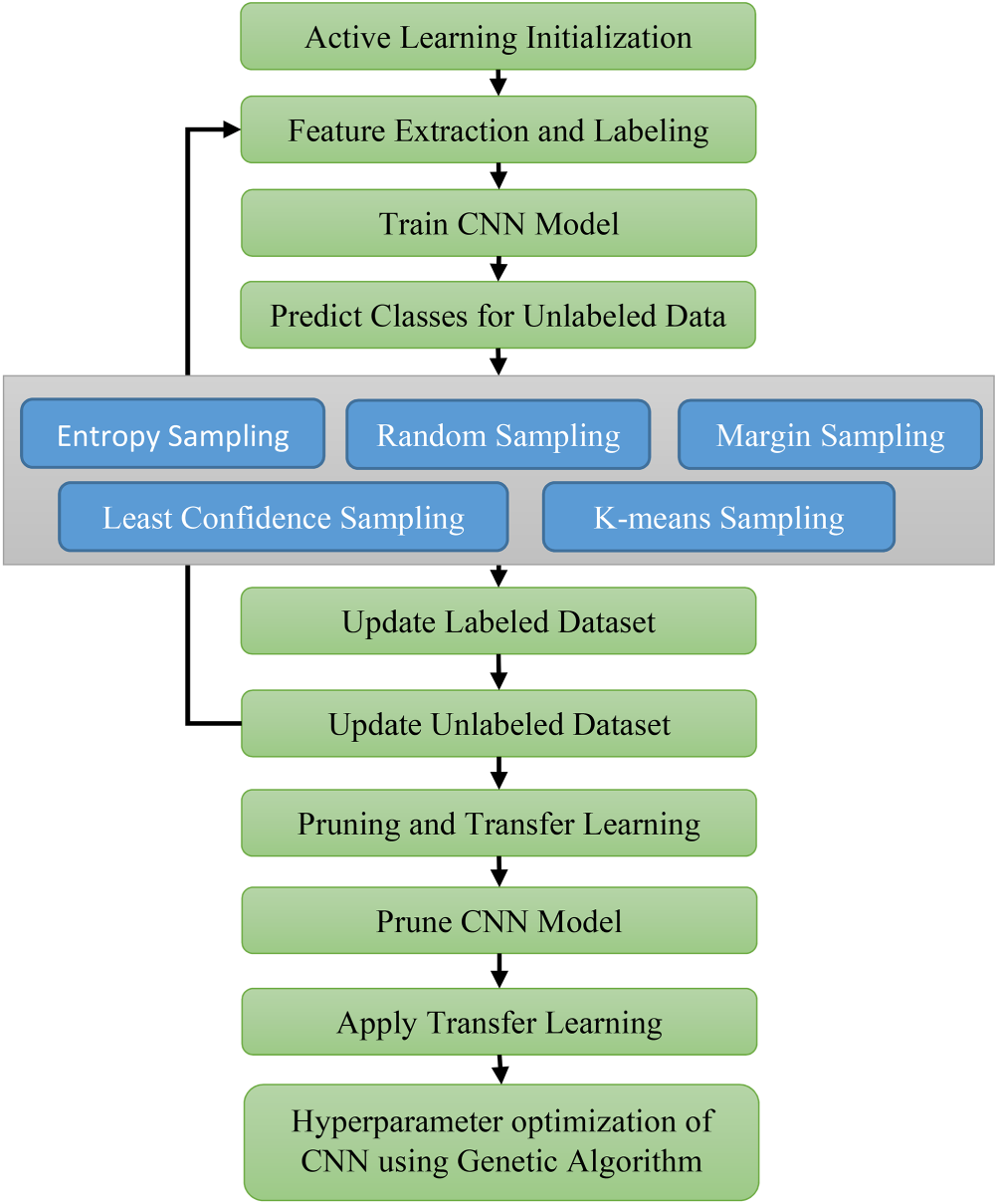
Overview of the proposed approach.
The essential tenet of AL is that a machine learning algorithm can perform better with fewer training sessions and data if it can choose the data it learns from. A model is frequently trained in a controlled learning system using thousands of labeled instances. These labeled cases may occasionally have a large amount of overlap. As a result, a different sample might improve the model's performance more than several samples of the same instance. The unlabeled data points chosen by active learning algorithms are those from which it anticipates the most significant improvement in the model. AL next requests the data point's label from an oracle. The labeled data point can be utilized in training, much like in supervised learning. The classic AL acquires labels one by one. However, this is not possible when training CNN because a single point will not have a statistically significant effect on the model due to the local optimization procedures; due to the size of many fundamental problems of relevance, it is impossible to train as many models as there are points. Therefore, a batch AL selects a large set of points labeled with each iteration in this study. At each iteration, AL identifies and labels data points and then classifies them using previous and newly labeled data points with the help of a classifier.
Least confidence sampling
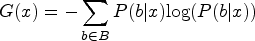
The LCS technique 7 is a method used in active learning that is aimed at finding and selecting the samples of which labeling is the most uncertain. It is a technique that enables the model to concentrate on the samples that it is not confident about, thus, the use of the labeling resources becomes more efficient and the training becomes more effective. The aim of least confident sampling is to identify the samples for which the model is most uncertain about its predictions. This is achieved by obtaining the difference between the highest predicted probability for each sample and 1.
In this technique, the uncertain samples are chosen. For example, there is a matrix, Tp,s, in which each column represents a sample and each row represents a class. For each sample, a vector Vc contains the probability of whether a sample belongs to a specific class ‘c.’ Then, the samples have a small max (Tp,s) for s € {1, 2, 3, …., i}, where i is the total number of samples queried. In a pool-based sampling scenario, the samples with the lowest confidence are picked to avoid the labeling cost. This technique takes the difference between 1 and the most confident predicted label, as shown in Equation 1.


The above equations is used to identify the samples with the highest values which are then given priority for labeling. This implies that the model is paying more attention to the data points on which it is less sure, thus making the greatest improvement in model performance possible when labeled. Through the selection of samples with the least confidence, the model will be able to focus the labeling efforts on the most uncertain data points and thus, more informative ones.
LCS in active learning effectively improves model accuracy by focusing on the most uncertain samples for labeling. This way of labeling is very effective in using the labeling resources and also improves the model with fewer labeled samples. LCS also minimizes labeling costs and time by focusing on uncertain samples, which results in faster enhancement of the model's performance and resilience. However, LCS can be computationally expensive and challenging to implement since it requires the determination of the confidence levels of each sample before comparison. Bias may occur in the model since it may overemphasize certain types of uncertainty at the expense of other areas of the dataset. The method's success depends on the performance of the initial model, and if the initial predictions are bad, they may lead to wrong sample selection and thus inferior learning results.
As a result of choosing random samples from a pool of unlabeled data for labeling, random sampling is a basic form of active learning. 8 There is no prejudice at all in the algorithm as it does not take into account any factor like model uncertainty or information, therefore the samples are selected randomly from the available set of unlabeled data. This is a type of random sampling technique that is regarded as simple and objective at the same time and is used as a reference point to compare other types of active learning. With random sampling, researchers can find the efficiency of novel strategies like the least confidence sampling and the entropy sampling against the simple and bias-free approach. Unlike other methods, that prefer a certain type of samples, random sampling is an impartial technique that treats all the samples uniformly, irrespective of their source. Thus, it can provide a fair assessment of how other methods perform about a completely neutral method. Random sampling may be easily implemented by the random selection process, for instance, using a random number generator to pick samples from the unlabeled pool. Because of its simplicity, it can be an easy-to-use tool where other active learning strategies may be too complicated or expensive. Testing the model on the data where the labels are randomly assigned gives the researchers an insight into the performance of the model without what is known as active learning. Meanwhile, this allows for assessing how well the other active learning techniques succeed.
Random sampling is easy to implement, requiring only a random number generator to select samples from the unlabeled data pool. It is unbiased, treating all samples equally without considering factors like model uncertainty. Serving as a neutral baseline, it allows researchers to compare the effectiveness of more sophisticated active learning techniques. Its simplicity makes it cost-effective and accessible for preliminary analysis, providing a fair assessment of how other methods perform in comparison. Random sampling is inefficient as it does not prioritize informative or uncertain samples, potentially requiring more samples to achieve the same performance as targeted methods. It does not leverage the model's uncertainty, leading to slower improvements in accuracy. While useful as a baseline, it offers limited insight into the learning process. The performance of models trained on random samples can be inconsistent, as the random selection may not capture the most representative samples. Thus, it is not an optimal strategy for active learning.
Entropy sampling
Entropy sampling
6
is an active learning technique involving the uncertainty of the class prediction to choose the sample. The method deals with the entropy information, which is the value of distribution uncertainty or unpredictability, to select the most uncertain samples from the unlabeled data set. The aim is to select the samples that will be most useful for the model when it is being labeled so that the model can be made to perform better. This technique is an uncertainty-measuring technique. In this technique, the user chooses a sample of labels having the highest-class prediction information entropy. Entropy is evaluated as follows:
The approach achieves it by choosing the samples with the highest entropy which means the samples with the many possible labels are going to be labeled. This approach is effective since it helps the model understand the data better by focusing on the areas where it is most in doubt. Thus, it enhances the model's capacity to generalize. Margin sampling which is also one of the methods is a procedure of selecting samples depending on the difference of odds between the most probable class and the second probable class. As the margin shrinks, the model will tend to misclassify the sample the more, the smaller the margin is. Margin sampling is expressed as in equation (4)
The idea was put into practice by Jimmy McQueen in 1967 (J, 1967).
10
This method serves to get rid of or find homogeneous data in a given dataset. Every homogeneous group is called a cluster, or area, in the N-dimensional space where the data points are closer to those regions. Every gathering has a centroid. From the points that are nearest to the centroid, the data points are picked for labeling. The distance is considered as the Euclidean distance as indicated by Equation 5:
K-means sampling 10 is a suitable method of selecting samples for labeling from the dataset because it groups similar data points and selects samples with proximity to the centroid of the group. This approach is useful for labeling as it only focuses on the most significant data points in each cluster, which in turn can improve the model's accuracy because the labels will be more reflective of the data. Since K-means sampling leads to the reduction of the variance within the clusters as well as the increase of the variance between the clusters, it helps in the creation of a well-balanced and informative labeled data set that is useful for the generalization and learning of the model. K-means sampling method may take a lot of time particularly when working with large data sets in that it requires many computations of distances and the recalculations of the centroids of the clusters. This process may also be sensitive to the initial placement of centroids which may be a disadvantage since it may at times produce poor clustering. Moreover, K-means sampling assumes that the points within the radii of the centroids are good samples of the clusters which may not be the case particularly when working with complex or jagged densities. This assumption can sometimes lead to the selection of less informative or less diverse samples for labeling which in turn can limit the improvement of the model.
A CNN is an instrument that allows image processing and image classification. It is composed of several convolution layers that are used to extract features from the images as opposed to operating on the entire image at once. CNNs are made up of an input layer, an output layer, and several hidden layers that enable the network to learn. To enhance the detection, in our study, we used a deep CNN with three layers of convolution. Convolution is a process of summing two mathematical functions which are useful in creating new features which are very essential in classification. Max pooling is a sample-dependent discretization process that reduces the complexity of the input representation used in the paper. This simplification enables decision-making that is more efficient due to the features of the binned sub-regions that are present. Figure 3 shows the working of our CNN model with max pooling as to how it works for feature extraction and image classification.
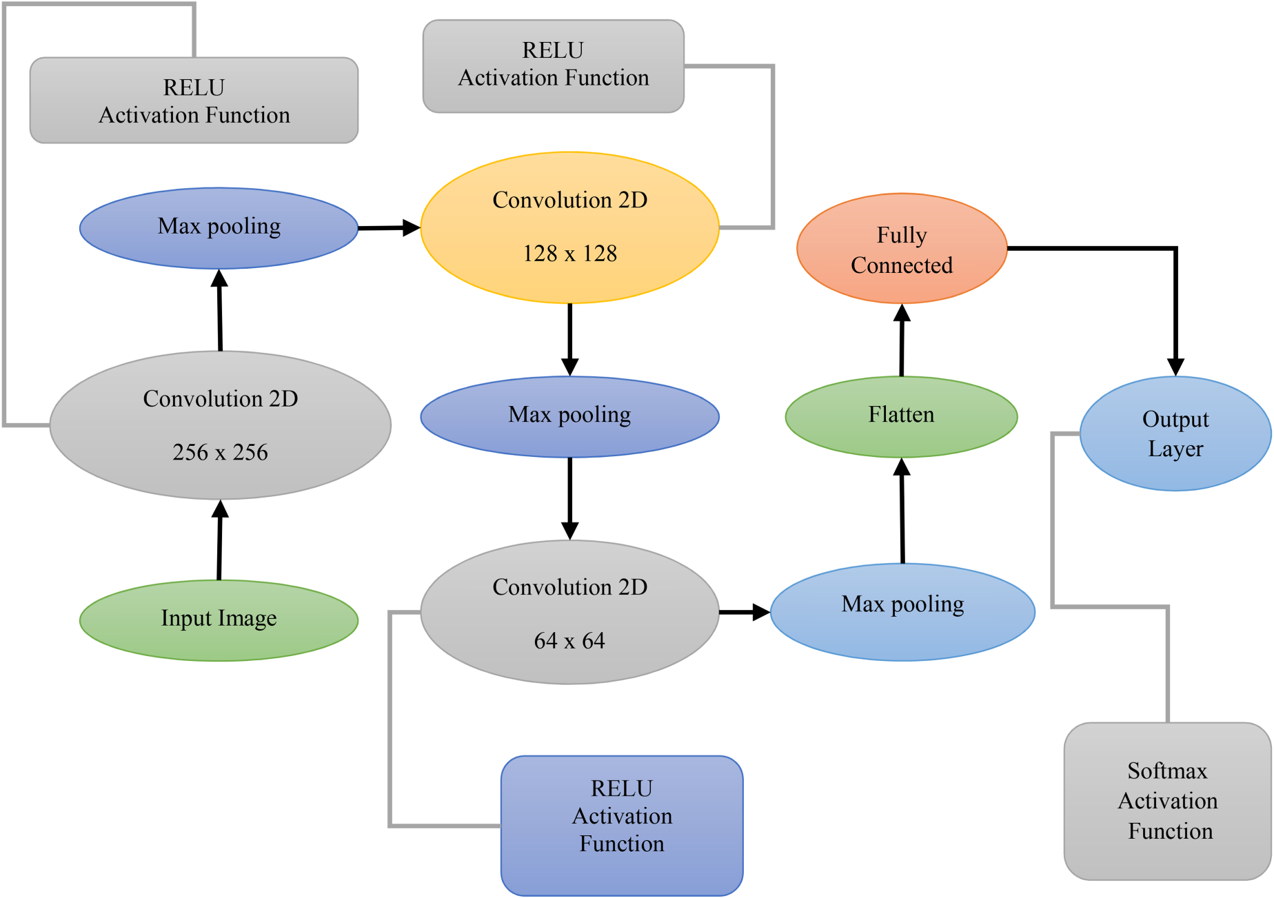
Three convolution layer with Max pooling operation.
CNN is used in image processing and the classification of the images. CNN is made up of one or more layers of convolution. Rather than dealing with a picture as a whole, CNN looks for aspects that work well inside images. CNN comprises an input layer, an output layer, and several hidden layers. We used a deep CNN with three convolution layers in this research. By mixing two mathematical functions, convolution aids in the creation of a new function. One sample-dependent discretization technique is max pooling. Reducing an input representation's complexity will allow choices to be made about the characteristics contained in the binned sub-regions. Figure 3 shows how our CNN model operates with Max pooling.
This time, an average pooling mechanism is used in addition to the same architecture for function mapping. Figure 4 depicts the model's activities. In average pooling, all values in the image matrix's area of interest are averaged, while in maximum pooling, the maximum value is taken in that region. We begin our CNN model using
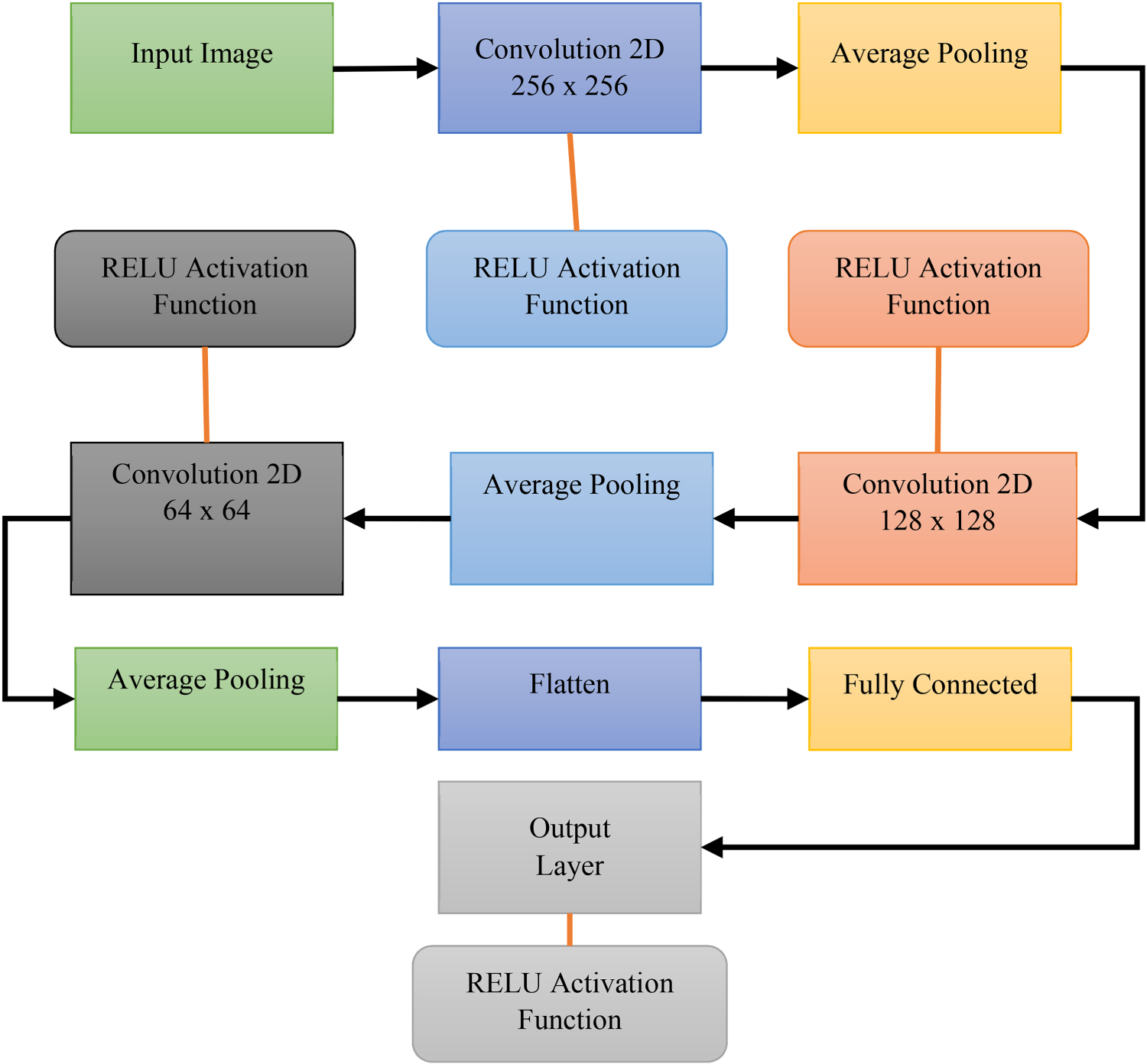
Three convolution layer with average pooling operation.
All the above-stated sampling techniques will be applied with CNN for face mask detection. The complete algorithm for AL with CNN is illustrated below, using entropy sampling techniques.
The active learning algorithm first selects a small sample of data that is labeled manually as presented in Algorithm 1. The model is trained on this small labeled data. Each unlabeled data set's class is predicted using this trained model. The sampling techniques come into account when choosing the data samples for labeling. Once the sampling technique is finalized, the selected technique is used to label the data. This algorithm selects two subsets, L1 and L2, from the dataset. L1 is the labeled set, and L2 is the unlabeled dataset. L1 dataset will increase with each round of iteration, and L2 will decrease with each round of iteration. Each experiment runs for a different number of iterations. On these subsets, all the sampling techniques are applied one by one. The model CNN is trained with the L1 dataset. Based on the sampling technique, the topmost samples among unlabeled data are chosen and sent to Oracle for labeling. Entropy sampling is used when the model is not confident enough for labeling. As this experiment proposes a novel transfer-learned pruned CNN model, it was assumed that the model might not be sure about labeling. Therefore, the entropy sampling technique is used. The results in section 4 also prove that the decision to use the entropy sampling technique is perfect.
Active learning-based CNNs offer several benefits compared to traditional CNNs trained on static datasets. Active learning allows for the selection of the most informative data samples for labeling. This means that instead of labeling the entire dataset, which can be time-consuming and expensive, only a subset of data points is labeled, leading to more efficient use of human annotator time and resources. Active learning permits the model to adapt to the variety of data distribution at different times. Iteratively, the active learning system can choose the most relevant data samples to label as new unlabeled data becomes available. So, the model will always be up-to-date and robust to changes in the environment. The scalability of active learning to large datasets and complex models is the possibility to perform training of deep CNNs on a humongous dataset without having to take a lot of time on the manual labeling of data. With the method of choosing only the most important samples for labeling, active learning can effectively cut the high annotation costs of large datasets. This is specifically for situations where you are dealing with big data sets, for example in computer vision or medical imaging, where labeling is labor and cost-intensive. Altogether, active learning-based CNNs provide a powerful and precise method by the way of selecting representative samples for labeling. Due to the capability of these models to accomplish high performance with fewer labeled examples, the development and deployment of deep learning systems are faster.

Pruning and transfer learning (TL) of CNN
The pruning process is one of the ways to reduce the parameters while at the same time leading to the diminishing of the detection accuracy of the model. A transfer learning technique is used to increase the accuracy of the algorithm detection. The proposed transfer learning algorithm is employed in this study to improve CNN's detection accuracy. Algorithm 2 provides the complete procedure which is used for pruning CNN.

Pruning is carried out to decrease the model's parameter count and speed up inference. The proposed pruning algorithm helps to adjust network depth and width. To restore the accuracy values lost during pruning, finetuning is also suggested in addition to the pruning process. During fine-tuning, the fully connected nodes where actual class label predictions are generated are deleted and replaced with newly initialized nodes. Finetuning also freezes older convolutional layers in the neural network to avoid the loss of any robust characteristics gained by convolutional layers. After the previous convolutional layers are frozen, newly initialized, fully linked layers are learned. All of the frozen conceptual levels are at last unfrozen. Algorithm 3 describes the transfer learning algorithm with pruned active-learned CNN.
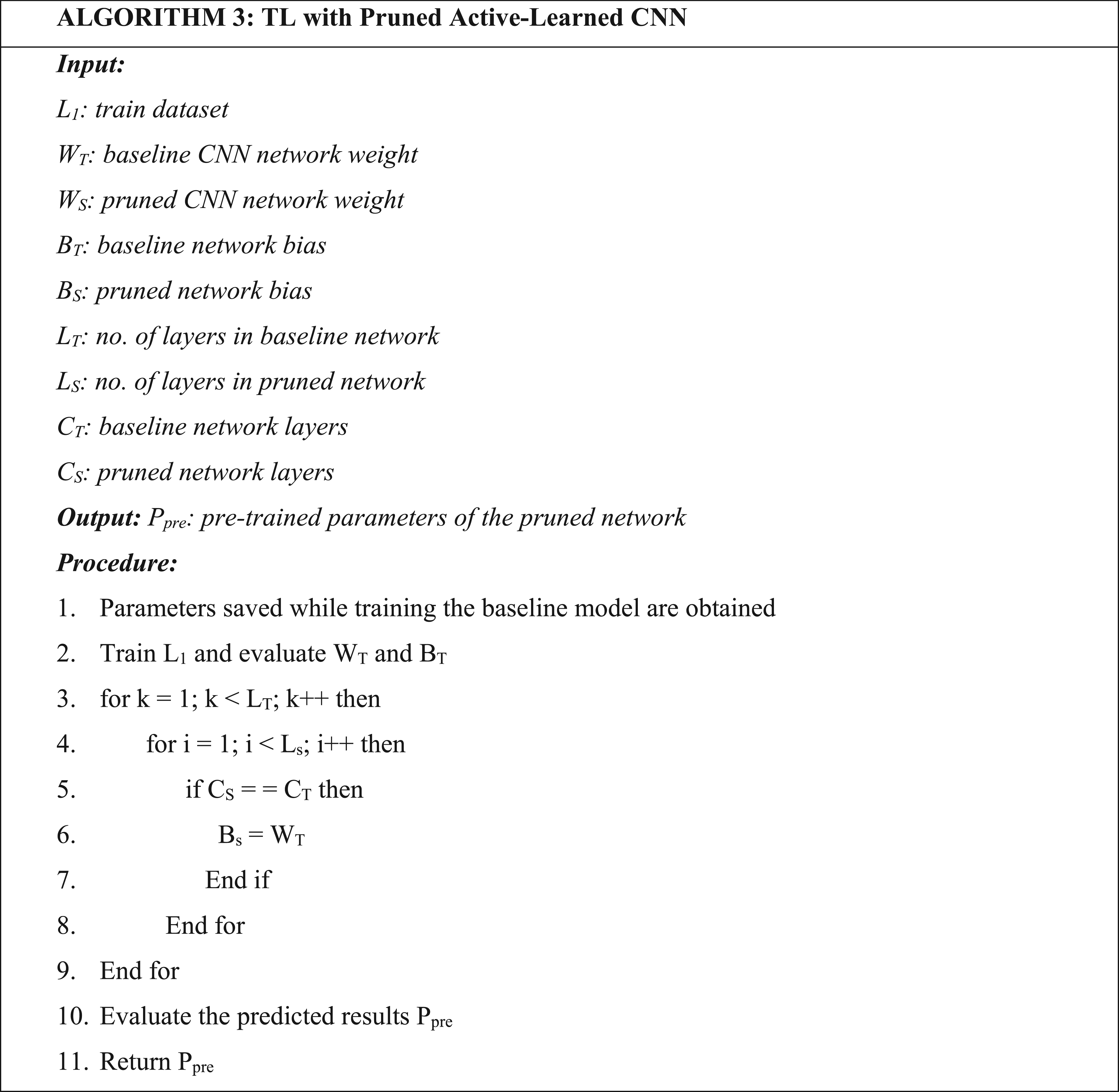
In TL, a student-teacher network of CNN is used. The weights and biases of the teacher network are used to initialize the student network. When baseline CNN and pruned CNN have identical channel counts, the teacher or baseline network weights are applied to the student or trimmed CNN biases. This approach enhances the model's general functionality as well as the model's ability to recognize objects more accurately.
Genetic algorithm-based CNN hyperparameter optimization
The trial was conducted manually, allowing us to identify a suitable fully connected layer design with an appropriate learning rate. Due to the time-consuming nature of these tests, we recommend using optimization methods. We selected GA 32 for this purpose. For both methods, we optimized the learning rate, the number of fully connected layers, the number of neurons per layer, dropout occurrence after layers, and dropout rates. The learning rate (LR) is represented as 10lr, where lr ranges from 1 to 6. The number of neurons per layer (fc) ranges from 3 to 10 and is converted to 2fc for the fully connected CNN layer. The dropout rate is a float between 0 and 0.6. Dropout layers are added after each fully connected layer, influenced by the algorithm's individual or particle definitions. These bio-inspired optimization strategies aim to identify an optimal architecture for fully connected layers with a satisfactory learning rate.
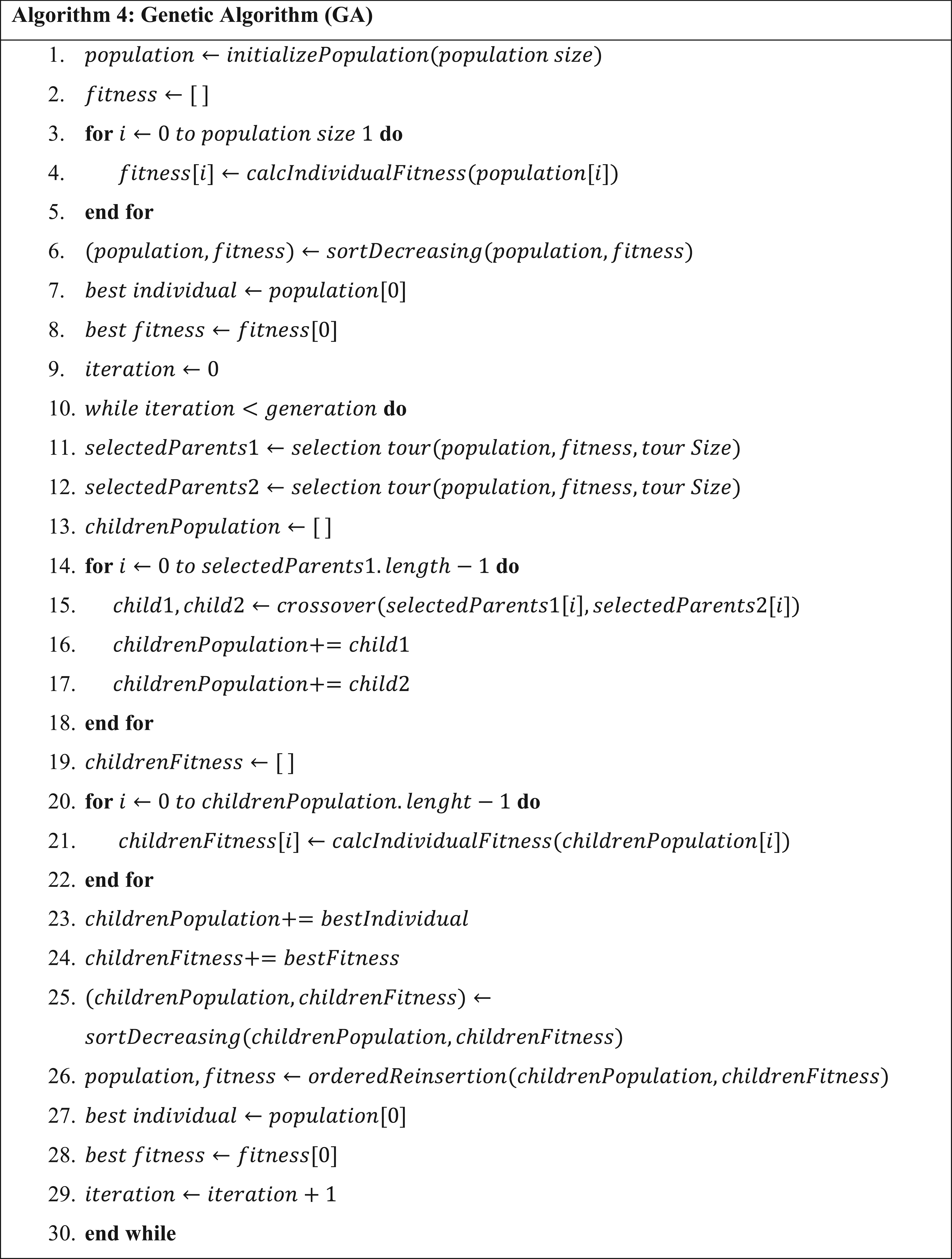
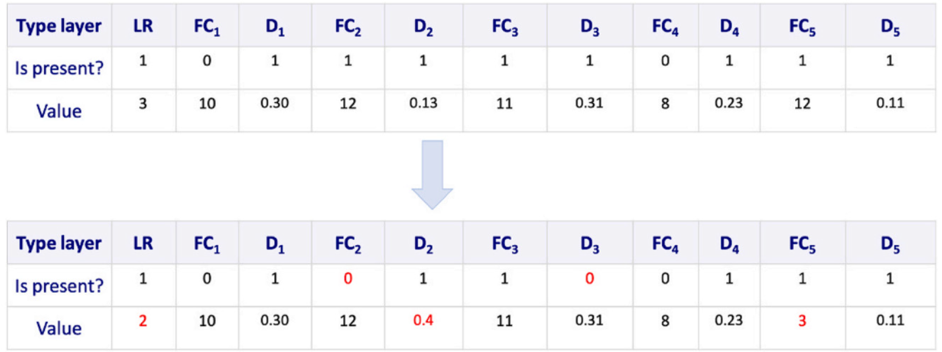
In this study, we use a similar approach to the optimization approach described in. 33 Each GA individual is defined with twelve chromosomes, each consisting of two sections: a flag indicating whether the chromosome can be modified (“Is present?”) and a value specifying the parameter or layer size. The learning rate is determined by the first chromosome. From the second to the eleventh chromosome, the odd chromosomes define dropout layers, while the even chromosomes define fully connected (FC) layers. To ensure the individual corresponds to a valid CNN, the final chromosome is always an FC layer with a value of 1, as 21 is the output of the CNN. This structure allows for precise optimization of the neural network architecture using GA, effectively balancing the flexibility and specificity of the model parameters.
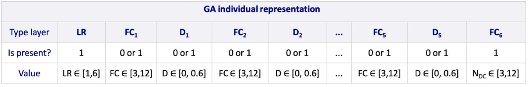
GA person definition.
In our GA approach, a dropout chromosome is ignored if the preceding FC layer chromosome has an ‘Is present?’ value of zero, as a dropout is only applied to the FC layer directly before it. There is a direct relationship between the number of FC layers and the number of ‘1’ values in the ‘Is present?’ flags for the FC layer chromosomes. To evaluate the effectiveness of the CNN architecture designed by the GA, we train the CNN and assess its performance using the F1-score on the validation set. During the experiment, we observed that some designs exhibited a non-decreasing number of neurons across layers, which is uncommon in CNN architectures. To address this issue, we introduced a penalty factor of 0.7 for architectures that showed a non-decreasing trend in the number of neurons from one layer to the next. For example, a configuration of 256 → 256 → 1024 is penalized, whereas a configuration of 1024 → 1024 → 256 is not penalized.

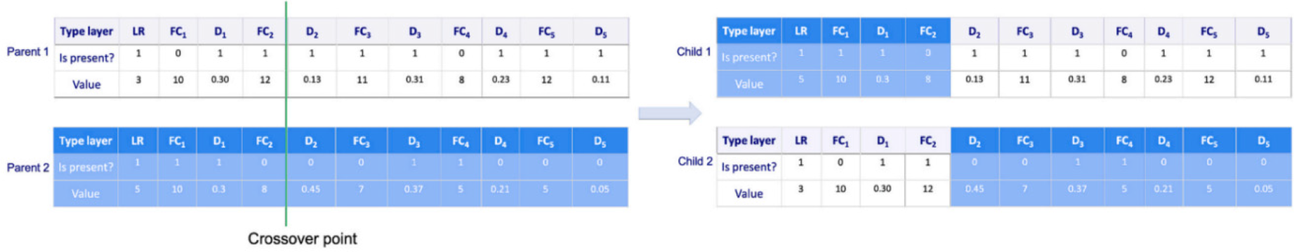
GA crossover.
GA individual mutation.
Experimental setup
The experimental setup for this study used Python 3.3 as the programming language on a system equipped with an 11th Gen Intel® Core™ i5 processor, 16 GB of memory, and Windows 11 as the operating system. With 145 GB of storage, the system managed datasets, models, and experimental results effectively. TensorFlow v2.13.0 served as the deep learning framework for developing and testing the CNN and implementing active learning techniques. The NVIDIA GTX 750 GPU was used to perform the computations for training the model and making predictions. This configuration made it possible to successfully develop, implement, and evaluate the proposed face mask detection methods.
The experiment concentrates on active learning, a procedure for choosing the most relevant data for training a model. The experiment is carried out with the help of PyTorch, which is an open-source deep-learning framework. To facilitate automated detection of mask usage, a dataset available on Kaggle provides 853 images categorized into three classes: “With Mask,” “Without Mask,” and “Mask Worn Incorrectly.” Each image is annotated with bounding boxes in the PASCAL VOC format, enabling precise localization of mask usage. This dataset serves as a valuable resource for developing machine learning models that can accurately identify and classify individuals based on their mask-wearing status, contributing to public health and safety measures. (Dataset Link: https://www.kaggle.com/datasets/andrewmvd/face-mask-detection/data). The goal is to create a classification model that can correctly predict these classes. The active learning process is cyclical and consists of five queries; at each query, the model chooses certain instances from the dataset to use for further training. The performance of the active-learned CNN is compared with two existing models: The Corona mask, a two-stage CNN developed by Gupta et al. for real-time face recognition, and a Yolov6 model fine-tuned by the same authors. The study evaluates the outcome of all five queries with the transfer-learned pruned CNN model. Transfer learning involves utilizing a pre-trained model and fine-tuning it on the specific task at hand. The efficacy of this approach in conjunction with active learning is evaluated. The study then compares the real-time face recognition performance of all three models. This comparison highlights the relative strengths and weaknesses of each approach in practical applications. During training, a batch size of 16 is used, along with the Adam optimizer. The input image size is set to 640 × 640 pixels to ensure compatibility with the chosen models. Training is carried out for 300 epochs to allow models to converge to optimal performance levels. The Kaggle dataset is partitioned into training and testing sets in an 80:20 ratio to facilitate model evaluation and validation.
Performance metrics
To evaluate the performance of each model, several key metrics are used:
Precision
Precision, in simple terms, tells us how trustworthy the model is when it predicts something as positive. It shows the percentage of correct positive predictions out of all the instances the model labeled as positive. High precision means the model is accurate in identifying positives, reducing the chances of wrongly labeling something as positive.
Thus, the model classifies people correctly into this group, out of all actual people in the dataset. It showcases the models’ ability to portray sensitivity in the detection of any particular class, which illustrates its capacity to pick out the relevant information.
This is the harmonic of precision and recall. It gives a generalized measure of the model's effectiveness, by considering both its tendency to make correct positive predictions and its capacity to evade false negatives.
This is a calculated measure, which, effectively, is the area under the precision-recall curve. It assesses the precision of the model at all recall levels of the operating points providing information about the performance level of the model at various points of operations.
This is the equivalent of the evaluated average precision computed across different classes. It is a world-scale statistic of the model's performance, considering its capacity to properly determine pictures of all categories. The highest mAP implies that the model exhibits excellent performance in terms of the accuracy of the recognition of images with masks.

The table shows the distinction in the models’ performances when they are trained with different learning rates and various amounts of labeled data. The accuracy rate is the main metric that demonstrates the performance of a model, and it is the percentage of correct predictions made by it. A model with a higher accuracy rate is performing better compared to others. The table shows that increasing the learning rate (the faster the model learns from data) makes the model better at prediction. Furthermore, as label data (already classified data) is increased, the model accuracy will improve. In other words, no matter what learning rate is used, this dilution effect is common, and hence training a model with more data (usually) makes it better to perform. Usually, the best results are generated when the learning rate is set to zero. 05 or 0. The rates are quite good at giving the model the ability to learn fast while also being precise. Now, as more labeled data is being gradually stuffed into it, the model becomes more and more perfect, but there comes a time when adding data does not make as impactful an improvement as before. Thus, not only the number of data samples and the learning rate are worth studying; however, but the model should be improved by analyzing other influencing factors. In general, the table shows that to achieve the finest results, one should make the right choice of learning rate and train on sufficient labeled data. More learning rate and data are indeed good for the performance of the model, nonetheless, the question is as to what extent we can improve the model by just using these factors. We will, therefore, need to look deeper at the other aspects of the model like as the choice of architecture and the training algorithm which may help to keep the progress going.
Table 2 provides a comparison of different LR and labeled LS using a random sampling technique. As seen in the table, at LR of 0.001 and LS of 1000, the accuracy is 0.117, while at LR of 0.05 and LS of 6000, the accuracy reaches 0.963. Analyzing the results, it's clear that increasing the LR generally leads to improved accuracy across different LS values, especially as LR progresses from 0.001 to 0.1. For instance, at LS of 7000, the accuracy rises gradually from 0.782 to 0.964 as LR increases from 0.001 to 0.1. Regarding the impact of LS on accuracy, it's evident that higher LS values tend to result in better accuracy for all LR settings. For instance, at LR of 0.01, the accuracy increases from 0.424 at LS of 1000 to 0.954 at LS of 7000. This demonstrates that having a larger labeled dataset contributes to enhancing model performance. The table demonstrates how LR and LS affect the model accuracy and the need to choose the correct LR and adequate-sized labeled data for training the models. It underscores the significance of finding a balanced combination of LR and LS to achieve optimal performance in model training.
Comparison of various LRs with different LSs using a random sampling technique.
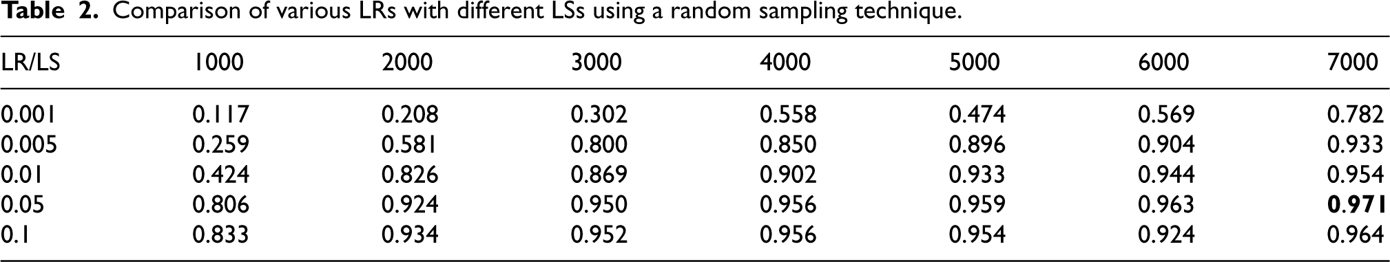
Comparison of various LRs with different LSs using a random sampling technique.
Figure 8 is a graphical depiction that shows the relation between the learning rates and the labeled sample sizes using random sampling. This number assists the researchers in determining the impact of the various learning rates and labeled sample sizes on the model accuracy and consequently, the researchers gain an understanding of the ideal parameter settings for the model training.
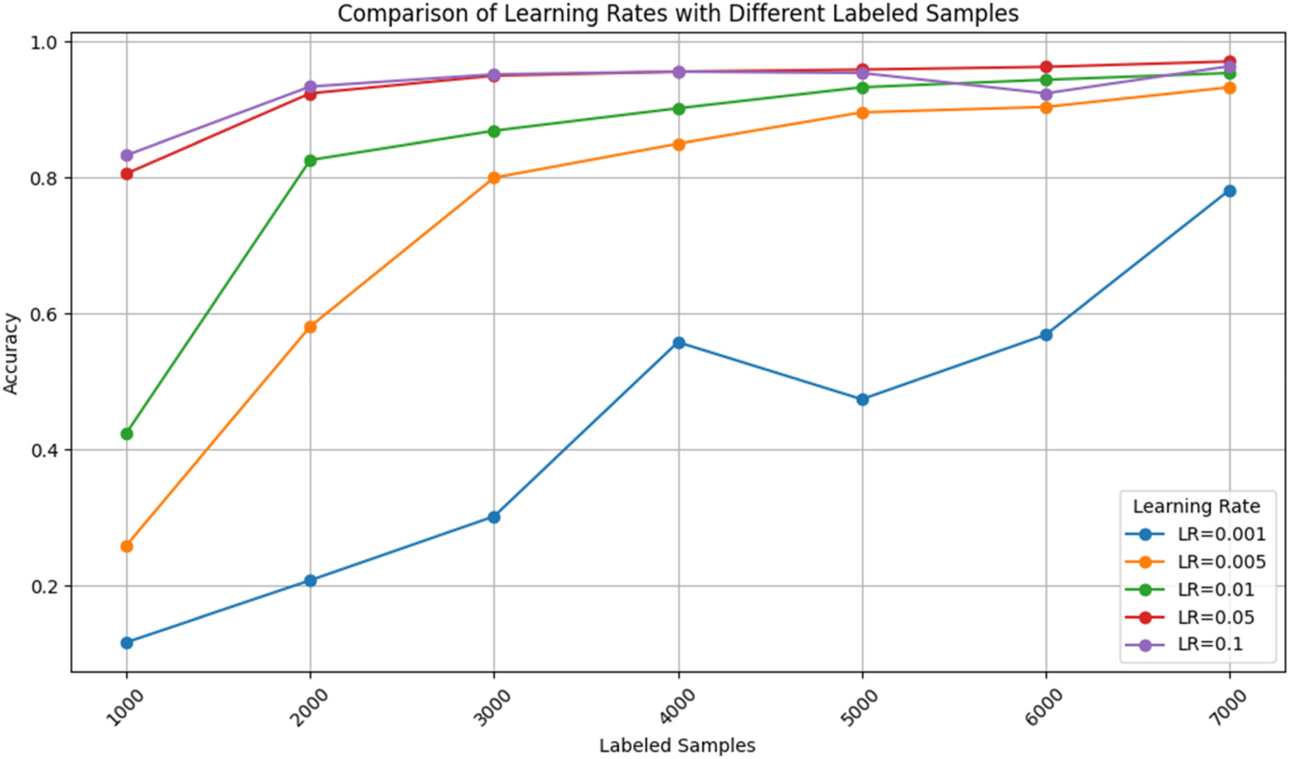
An accuracy comparison with different learning rates and labeled sample sizes using random sampling.
Table 3 offers a detailed comparison of different LR with varying LS using the least confidence sampling technique. Each LR represents a specific value ranging from 0.001 to 0.1, while each LS indicates the number of labeled samples, ranging from 1000 to 7000. A prominent trend observed in the table is the positive impact of increasing LS on the model's performance across all learning rates. Usually with an increase in the number of labeled samples, the model gets better, meaning the accuracy score increases and the performance metrics improve. This fact is common for all values of LR. For example, at LR of 0.002, it is seen that the model performance improves along with the increase of the LS from 1000 to 7000. Accuracy scores are on the increase from 0.116 to 0.782, the model is demonstrated as having more power of prediction with more labeled data. The table highlights how the different LR values affect the models’ output as well. LR of 0.1 consistently brings the accuracy scores to a high level for different LS values, demonstrating that it is capable of learning with the labeled data. Conversely, LR of 0.001 and LR of 0.005 seem to have slightly lower accuracy scores, especially with fewer samples for being labeled, hinting at the requirement of more data to have a minimum acceptable performance. Fundamentally, the table gives important inference which is the relationships between learning rates, labeled samples, and model performance with the help of the least confidence sampling approach. This is because it highlights the importance of choosing the right LR and LS values to improve model performance for specific tasks and datasets; which makes increasing labeled data a great thing for accurate model and good generalization.
Comparison of various LR with different LS using the least confidence sampling technique.
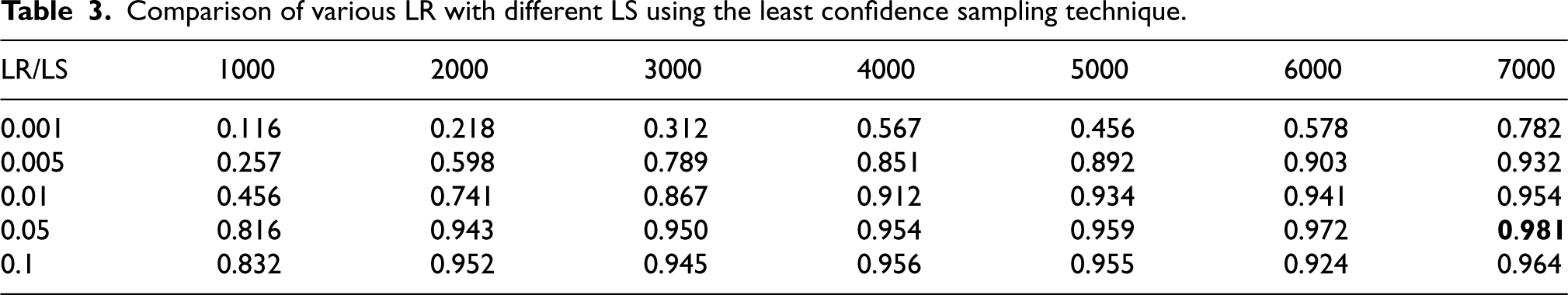
Figure 9, on the contrary, stands as a line graph that shows the learning rates with different sample sizes that are labeled using the least confidence sampling technique. How the differing learning rates, the sample sizes, and the model accuracy are charted, researchers can be able to see how the least confident sampling technique affects the model performance under different conditions.
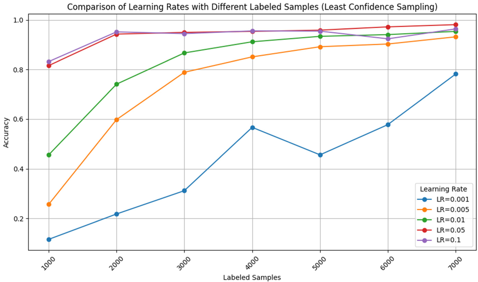
Accuracy comparison with various learning rates with different labeled samples using the least confidence sampling technique.
Table 4 constitutes a comparison of different LRs with different LSs, which has been carried out using the principle of entropy sampling. The data shows a key pattern that with the rise in the number of LS, the model performance gets better in all learning rates. This is signified by the fact that the accuracy scores improve as LS grows. For example, at LR of 0. 001, the model's accuracy develops as LS rises from 1000 to 7000. Precision jumps from 0.118 to 0.782 gave evidence that the model performed better with more labeled samples. The results address the matter of the response of the model to different LR coefficients. LR of 0.1 demonstrates a high accuracy of LS values consistently across all the labeled data settings, which means that learning from labeled data is efficient for it. In contrast, LR of 0.001 and LR of 0.005 are less precise, particularly with fewer marked samples, meaning that they need a lot of data to optimize their performance. Briefly, these are the major conclusions of the table concerning the interplay of learning rates, labeled samples, and model efficiency through entropy sampling. It implies that one can get better results by choosing the correct LR and LS values for the chosen tasks and datasets. It also underlines the possible use of annotation to improve the quality and increase of data which, in turn, facilitates the increase of model accuracy and generalization.
Comparison of various LR with different LS using an entropy sampling technique.
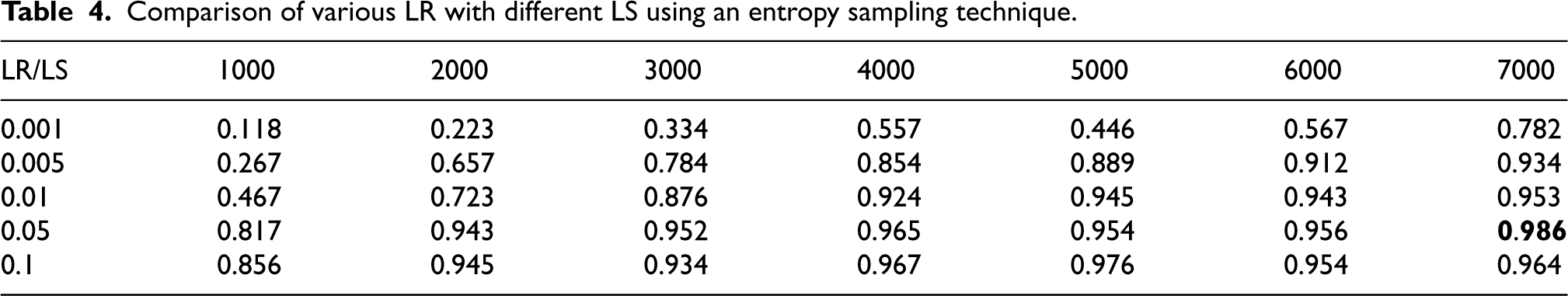
Even as in the case of Figure 10 which is a line graph that depicts the variability in learning rates with the entropy sampling method indicated by the sample sizes. This graph assists in figuring out the degree to which the entropy sampling approach is impacting the model accuracy at different parameters, consequently, researchers can discover the best scheme for training machine learning models.
Accuracy comparison with various LR with different LS using an entropy sampling technique.
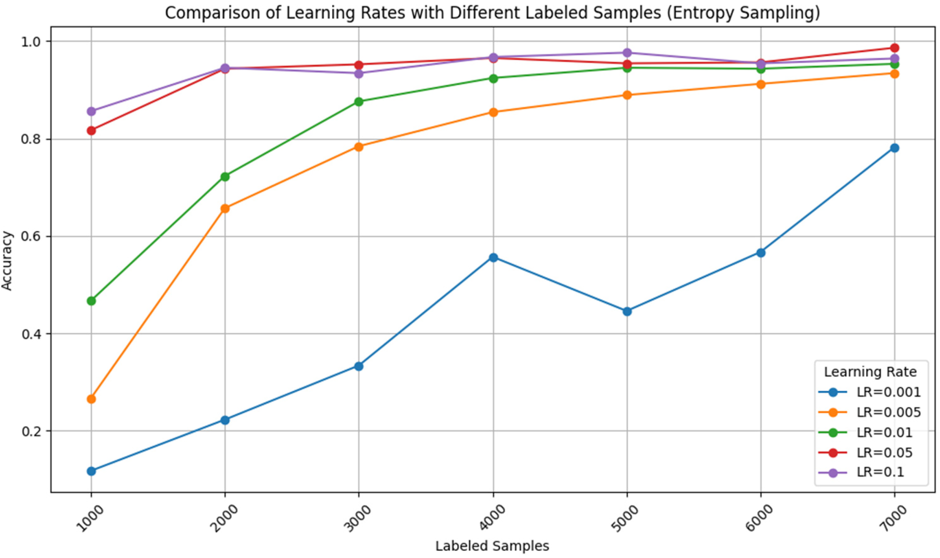
Table 5 shows the comparison of different LR with mixed LS sizes using the margin sampling method. We encounter the downfall of our model's performance when involving either of different LR and LS combinations. The variability points out the impact made by the choice of LR and LS on the accuracy of the model predictions using the sampling method based on the margin. For example, at LR of 0.001, the performance also depends on values other than LS. Usually, LR values with a higher score led to a higher accuracy, but the optimal LS may differ. Moreover, we discover that the model's performance is either at a plateau or declines as the LR gets very high, most likely in combination with the LS. This fact points out a possible drawback of using a large number of labeled data versus learning rate, thus, this relation should be carefully managed to have a positive effect on the model performance. In the end, the table shows the importance of picking the LR and LS numbers carefully and the margin sampling method as the factors that determine the model's performance. It underlines the need for trying different approaches and adjusting things until you find the right combination for a specific dataset and mission. It demonstrates the complex interaction between the learning rate, number of samples with labels, and model success, thus, the need for intense analysis and interpretation in machine learning experiments.
Comparison of various LR with different LS using a margin sampling technique.
Figure 11 shows the information that the margin sampling method affects the model performance by different learning rates and the number of training samples. Through the visualization of the relationship between these parameters and the model accuracy researchers can evaluate the efficiency of the margin sampling technique regarding the improvement of the model performance in various situations.
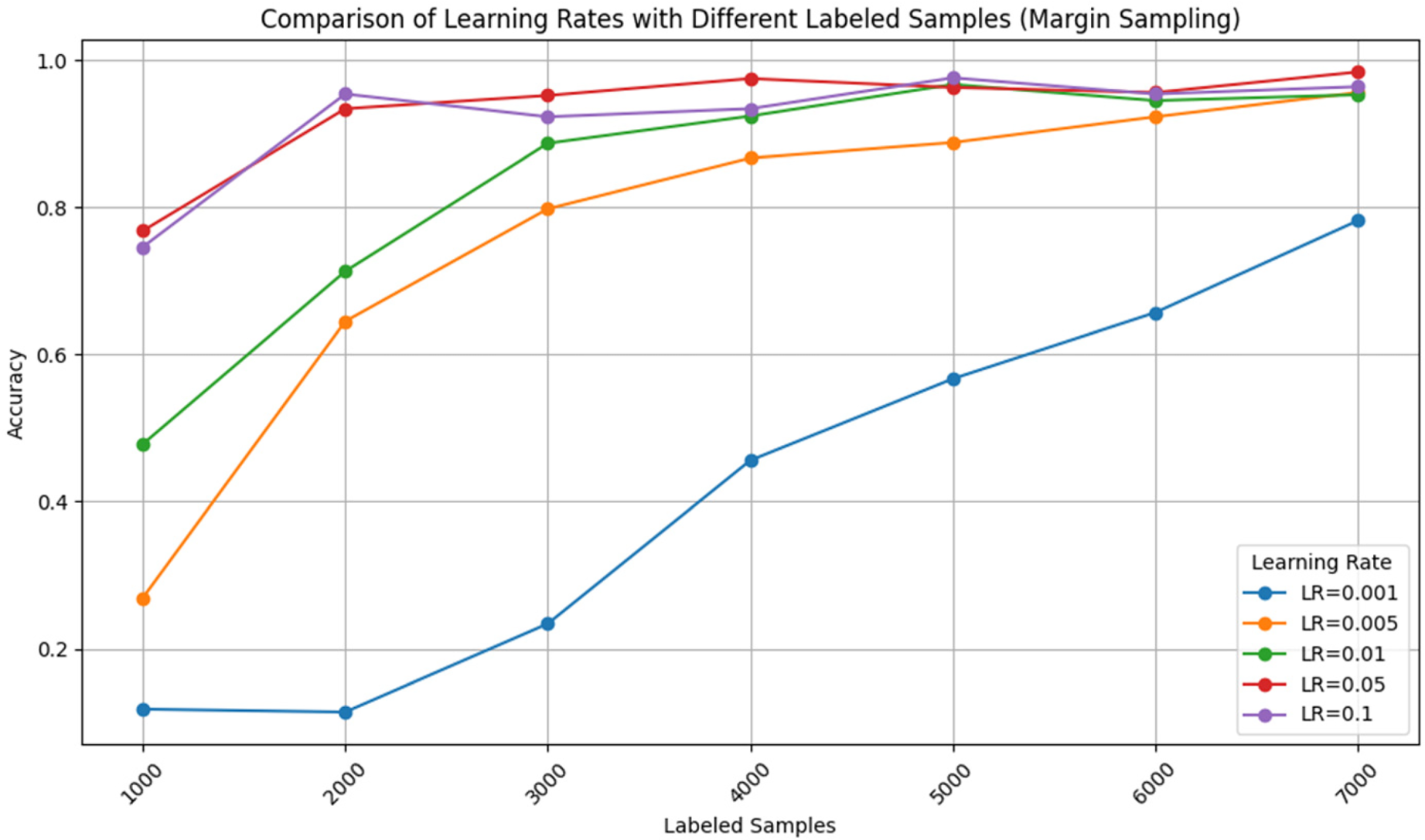
Accuracy comparison with various LRs with different LSs using a margin sampling technique.
Table 6 compares different LR with varying labeled LS using the k-means sampling technique. LR ranges from 0.001 to 0.1, while LS varies from 1000 to 7000. As seen in the figure, several key observations emerge. As the number of LS increases, there is a general trend of improvement in model performance across different LR values. This improvement is particularly noticeable for lower LR values. For example, at LR of 0.001, the performance shows a consistent improvement from LS of 1000 to 7000 with the accuracy scores increasing from 0.117 to 0.782. This fact is observed for all k values, which means that better performance can be achieved if more samples with the labels are to be used. Moreover, the influence of the LR on model performance is significant. High LR values, such as 0, indicate the most immediate needs. Relatively low LR values, such as 1.05 and 0.1, often prove to be more accurate in practice compared to other LR estimates. Conversely, the rate of advancement could be different as LR value and the details of the LS configuration, would affect how fast it improves. Additionally, the k-means sampling method shows good performance for different LR values as well as different LS configurations and has accuracy scores always above 0. 9 for most scenarios. This seems to mean that the k-means sampling method capable of choosing the informative points for the training of the model notwithstanding the changing of LR and LS settings. The accuracy performance of the model is shown in Figure 12 for learning rates with different sample sizes labeled but applying the k-means sampling approach.
Comparison of various learning rates with different labeled samples using a k-means sampling technique.
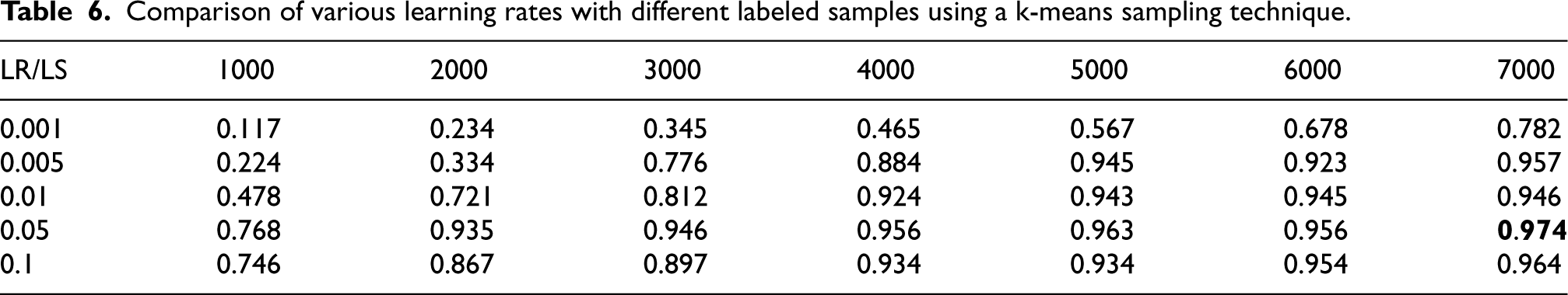
The performance of a model trained with different LRs across various LS sizes, using the k-means sampling technique.
In this section, a detailed comparison is carried out among three face mask recognition models: there was a pre-trained transferred pruned CNN, the Coronamask two-stage face mask detector. The evaluation includes using the dataset with labeled pictures illustrating people while wearing masks in diverse settings and live image streams from a webcam. The main purpose is to measure the model performance utilizing precision, recall, F1 score, average precision, and mean average precision metrics. This analysis covers also real-time settings, which means that researchers can assess their performance in dynamic and uncontrolled settings. The researchers can do so by watching the images that are captured on the spot directly and thus, find out the accuracy of the models in real-time. The assessment of the models on already existing datasets and real-time streams allows one to obtain insights into their strengths and weaknesses in practical use considering factors such as the level of their accuracy, speed, adaptability in different conditions, and the degree of their overall performance in real-life situations. The key takeaway here is that information in this description should be used in model selection and deployment for public health surveillance, security surveillance, and compliance enforcement, all of which should contribute to public safety and general wellness. Table 7 highlights the precision values for all the three models.
Results of all compared three models.
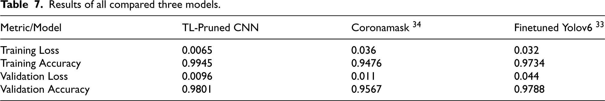
Results of all compared three models.
Table 7 outlines the training and validation outcomes of three distinct models: TL-Pruned CNN, Coronamask, and Yolov6 finetuned with four metrics: training loss, training accuracy, validation loss, and validation accuracy. The model was set off with the TL-Pruned CNN, consequently, the training loss was impressively low, 0. The accuracy of training more or less 65% implies that it is quite close to the ground truth. The prototype showed a very high training accuracy of 99.45% which demonstrates the effectiveness of learning from the training data. The TL-Pruned CNN demonstrated this in the validation step by having a low validation loss of 0.0096 and getting a validation accuracy of 98.01% which shows good generalization performance on unknown data. Considering the following model, the Coronamask, the training loss was slightly higher with the value of 0.0.36 as opposed to the 0.44 of TL-Pruned CNN, which shows that the propensity for losing accuracy is slightly higher during training. On the other hand, the training accuracy of 94 means that this model is eventually more likely to make accurate predictions. Accessing the ROC curve, the algorithm showed a 76% aptitude for learning from the training data. The Coronamask model validation reveals 0 loss. The result showed the performance of the model at 011 and a training accuracy of 95. 67%, meaning the satisfactory generalization capacity, though it is not the highest, yet slightly lower than the performance of TL-Pruned CNN. Next, we saw that the training loss of the yolov6 model is 0. 032 while the training accuracy is 97. 34%, which shows that during the training period overall stability had improved. Although the validation loss was higher qualitatively it only amounted to 0. As the RMSE value shows 044 compared to the other models, it details the likelihood of overfitting or worse generalization. Although Its validation accuracy of 973 out of 88% was average rank and not better than the performance of a CNN whose TL-Pruned Network was predicted. To sum up, the T-CNN model with the smallest weights and the highest activation showed the highest performance, having the lowest training and validation losses and the highest accuracy. The Coronamask model had its shape exactly like the Finetuned Yolov6 model, but, although the latter was still performing well, there was an indication of the possibility of overfitting in the latter during validation.
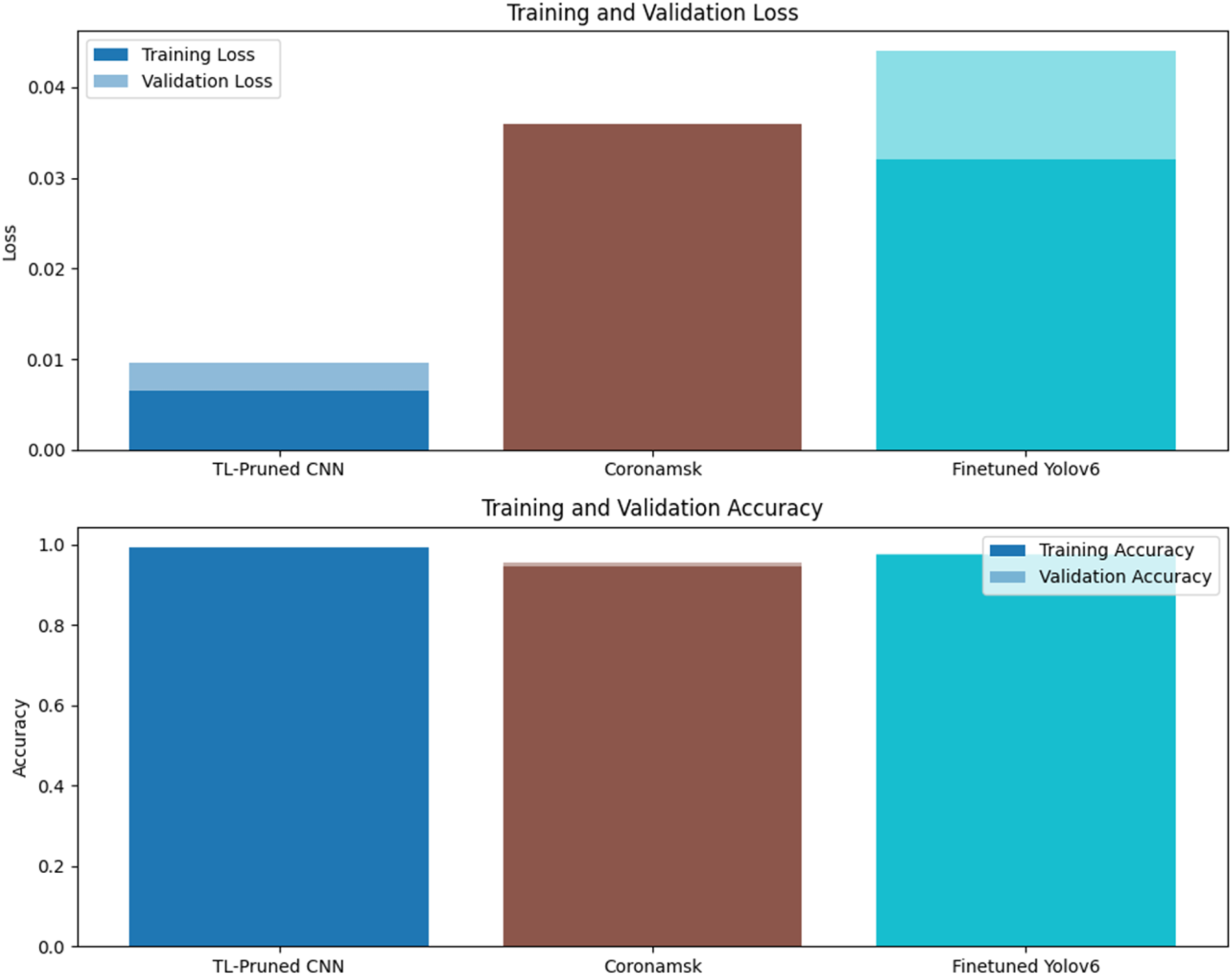
Accuracy results for the three models. TL-Pruned CNN, Coronamask, and Finetuned Yolov6.
Moving beyond training and validation, Figure 13 displays the accuracy results for three different models: TL-Pruned CNN, CoronaMask, and Finetuned Yolov6. Thus, the visualization allows the researchers to compare the performance of these models by their accuracy scores, thus, they can find out the strengths and weaknesses of these models in the face mask detection tasks.
When looking at the performance metrics of TL-Pruned CNN, Coronamsk, and Finetuned Yolov6, it's clear that TL-Pruned CNN outshines the other models. TL-Pruned CNN excels in precision, recall, F1-score, and mAP, demonstrating its superior overall performance. Coronamsk follows closely but consistently lags behind TL-Pruned CNN. Finetuned Yolov6, while decent, falls behind both TL-Pruned CNN and Coronamsk, especially in terms of F1-score and mAP. In summary, TL-Pruned CNN emerges as the top performer, with Coronamsk in second place and Finetuned Yolov6 in third based on these evaluation metrics Table 8.
Figure 14 goes on to the analysis of the three models’ performance by presenting the precision, recall, F1-score, and mAP metrics. This graph permits researchers to evaluate the models’ performance comprehensively and to find out which model is better in different evaluation metrics.
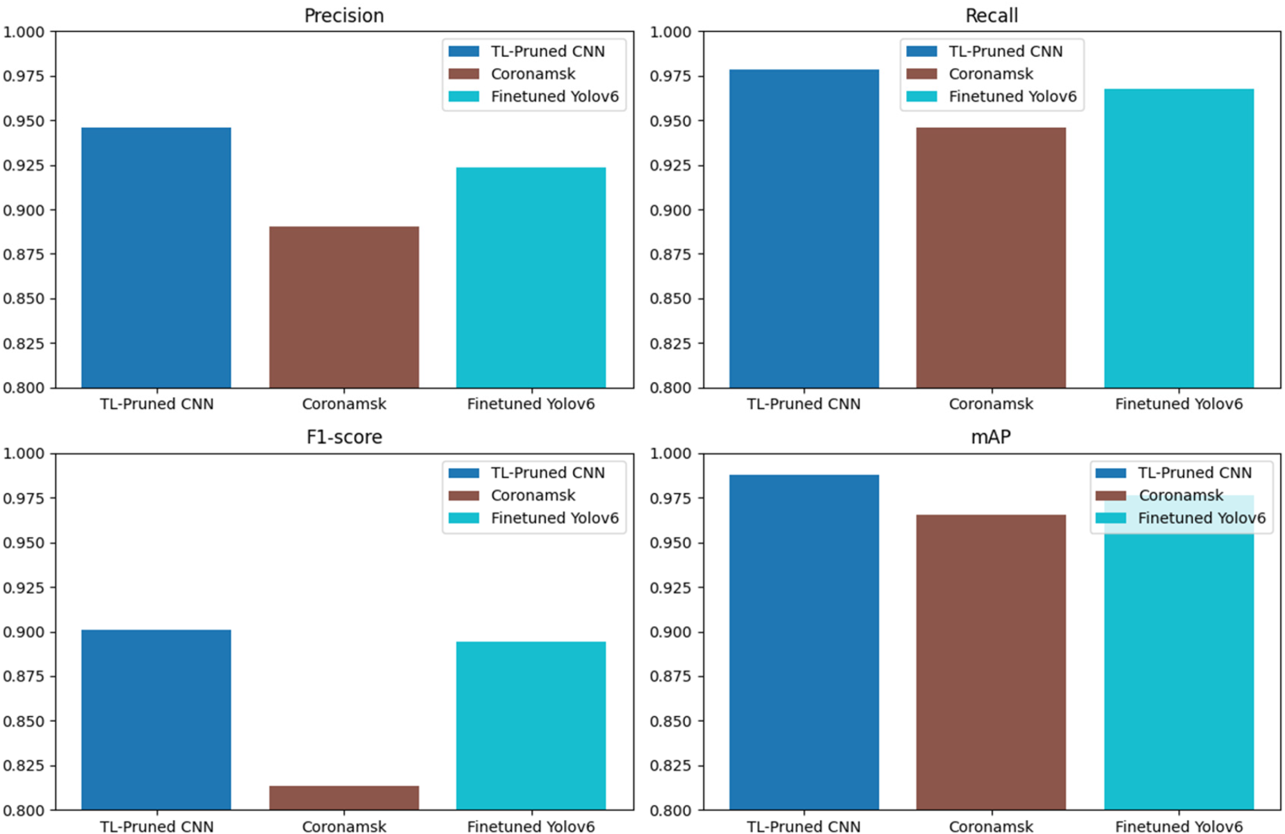
Figure 15 compares the models’ performance in real time through the use of YouTube videos. Through the presentation of the model evaluation results in a real-life situation, this figure provides valuable information about the practicality of the models for tasks like public health monitoring and security surveillance. In a nutshell, these visual representations are very important in the process of the interpretation and the understanding of the experiment results, hence, researchers can make the right decisions and the advancements in machine learning for face mask detection.
The meaning of these findings is not only limited to the evaluation of the model, but also it is a source of valuable information for real-world applications like public health monitoring and security surveillance. Through the analysis of models in dynamic and uncontrolled environments, researchers get a better idea of their strengths and weaknesses, which means that they can make the right choice in the selection and deployment of the model. The experiment results of this study will contribute to the advancement of machine learning in face mask detection. In this way, the researchers gain important insights into the model performance, parameters, and real-world applications, which help in the advancement towards the improvement of the face mask detection systems.
Performance evaluation of all models.
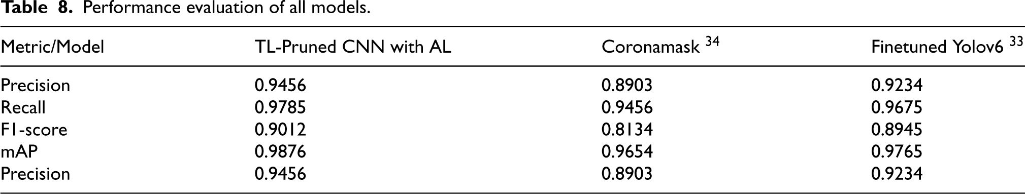
Performance evaluation of all models.
Comparative analysis of the precision, recall, F1-score, and mean average precision (mAP) with existing models.
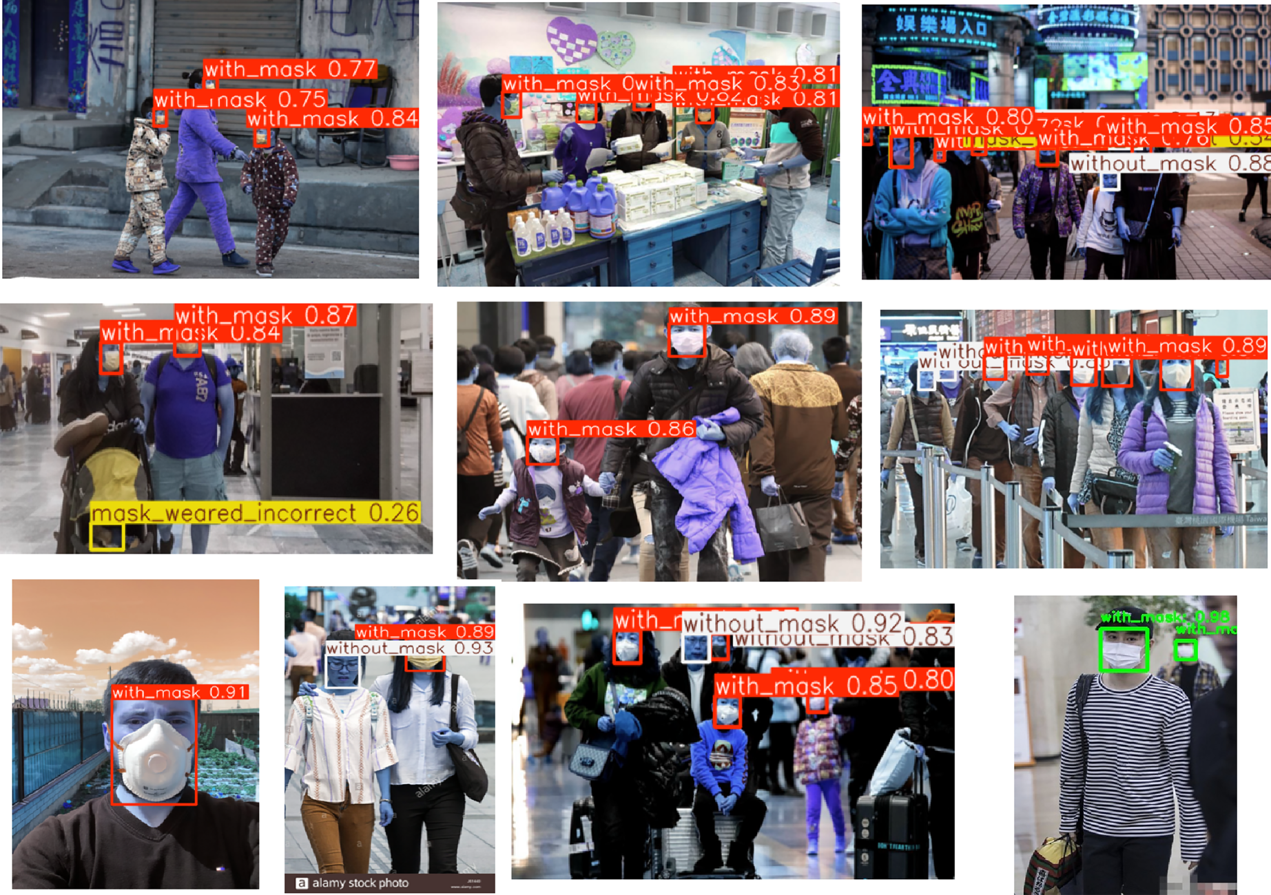
Face mask detection accuracies for different images using TL-Pruned CNN with AL.
Entropy sampling is one of the AL methods that greatly improves the model accuracy by directing the learning process to the most informative samples. As for the results, this study proves that choosing high-uncertainty samples along with transfer-learned pruned CNNs is more effective than the random sampling approach, proving the effectiveness of the proposed data selection strategy. Random sampling is used as a reference point because it is easy to implement and has no bias; thus, researchers can compare it with other strategies and determine the extent of enhancement. This goes to show that the more advanced the AL techniques, the better the performance of the model.
When applied to CNN models, pruning can help in the reduction of the number of parameters and the depth of the network which in turn increases the efficiency and shortens the time of inference. However, this process results in a reduction of the detection accuracy. To overcome this, fine-tuning is applied which involves replacing fully connected nodes with new nodes training them from scratch, and freezing and un-freezing some of the convolutional layers to maintain the robust features learned during the initial training. 35 The use of transfer learning increases accuracy even further because the pruned network is started with weights and biases from a well-trained base model. Balancing pruning for efficiency and mitigating accuracy loss is crucial, as it aims to maintain high performance while optimizing computational resources, ensuring the model remains both effective and efficient. 36
The practical implications of the study are huge, and they can effectively deal with real-world problems emerging from the pandemic. First of all, by applying the deep learning method the problem of automatizing mask detection for the benefit of public health authorities and institutions is resolved and so compliance with the mask policy is controlled. The application of CNNs which are known for their high accuracy in image classification can help the system to determine the individual's wearing masks in public spaces like transport, commercial establishments, and schools. This capacity is indeed most important to implementing mask-wearing mandates successfully and limiting the risk of transmission by a large number of people in highly populated public spaces.
Thus, building the simulated model training around active learning provides an advantage in the areas of streamlining and resource management. Through active learning, this method labels the most important data points selectively, thus requiring fewer annotations to build the model. In this way, the limited labeled data is used more efficiently. This efficiency becomes extremely essential in cases where one may not be able to assemble a large number of annotated datasets in a practical or resource-constrained manner. Therefore, the employed active learning approach widens the scalability and accessibility of the face mask detection machine, making it a more implementable system than a simple feed-forward one.
Limitations
This research work has drawbacks. Though the model shows good performance on benchmark data, it is still unclear if the method will perform well on real-world datasets with diverse scenarios because of the possibility that the data may be biased. It should be also mentioned that scalability and deployment issues may hamper the practical implementation of this approach in a variety of contexts demanding the consideration of computation resource needs and privacy protection implications.
Conclusions
This paper proposes a unique face mask detector that is more reliable and effective by further improving the two-stage detector using active learning, pruning, and transfer learning techniques. The active learning technique works on five queries, namely, least confidence sampling, entropy sampling, k-means sampling, random sampling, and margin sampling. Out of these five AL techniques, entropy sampling provided the most appropriate results. A dataset from Kaggle that was broken down into three categories: “mask,” “incorrectly wore a mask,” and “no mask” was used to train the models. For real-time verification of all the models, YouTube videos were employed. YouTube videos were used for extracting frames from them, and then classification was done with the help of models. Performance was measured using precision, recall, F1 score, average precision, and mean average precision. Comparisons were made with the CoronaMask and a fine-tuned Yolov6 model. Results indicated that higher learning rates and larger labeled sample sizes generally improved model accuracy. The TL-Pruned CNN demonstrated superior performance with a training loss of 0.0065, training accuracy of 99.45%, validation loss of 0.0096, and validation accuracy of 98.01%. The study underscores the importance of optimizing learning rates, sample sizes, and model architecture for enhanced accuracy in real-time face mask detection applications.
Future research will explore more advanced sampling methods such as Bayesian optimization, reinforcement learning-based sampling, or hybrid approaches that combine multiple sampling strategies could be investigated to further enhance model performance.
Footnotes
Author contribution statement
Adel A. Alyoubi worked solely on the manuscript.
Funding
The author received no financial support for the research, authorship, and/or publication of this article.
Declaration of conflicting interests
The author declared no potential conflicts of interest with respect to the research, authorship, and/or publication of this article.
Availability of data and materials
The data that support the findings of this study are available on request from the corresponding author.
References
