
Abstract
As the secondary ship market becomes increasingly active, achieving precise ship valuation while fully accounting for market fluctuations has grown increasingly important. This paper establishes a price assessment framework integrating static valuation with dynamic market adjustments: the static component employs an ACO–FA-optimized BP neural network to derive benchmark prices based on individual vessel characteristics; the dynamic component constructs a price index combined with oil prices and freight rates into a multivariate time series. A GRU model captures market adjustment factors, which are then fused with static valuations via Kalman filtering to generate final transaction prices. Empirical results based on Chongqing's 2020–2025 dry bulk carrier transaction data demonstrate that this model significantly enhances second-hand vessel price assessment while simultaneously delivering static valuations, market adjustments, and composite prices. It provides buyers and sellers with a well-explained quantitative basis for pricing, negotiation, and investment decisions across varying market conditions.
Introduction
As the global shipping market gradually recovers, the pace of vessel replacement accelerates, drawing significant attention to the activity and price trends in the second-hand ship trading market. Compared to the lengthy construction cycles and high costs of newbuilds, secondhand vessels offer advantages such as shorter delivery times and flexible pricing, making them a key option for corporate asset allocation and fleet capacity adjustments. However, ship transaction prices are influenced by multiple factors including vessel age, tonnage, market freight rates, and macroeconomic fluctuations, resulting in significant volatility and uncertainty. 1 Without effective evaluation mechanisms, enterprises often face information mismatches and judgment biases in critical decisions such as “whether to purchase” and “when to purchase,” potentially leading to increased costs or investment losses. Therefore, developing a price prediction model that integrates both static vessel characteristics and dynamic temporal trends holds significant practical importance. It offers urgent application value for enhancing corporate risk management capabilities and market responsiveness.
Machine learning methods have been widely applied in valuing secondhand assets like ships, automobiles, and real estate. Zhang Xinyue and Xiang Xuanyi demonstrated that in predicting used sailboat prices, the Random Forest regression model achieved the highest accuracy, with hull length emerging as the most significant price determinant. 2 Bal et al. employed a four-stage machine learning workflow to evaluate ultra-large vessels, ranking the XGBoost model as the top solution. 3 Zhao Jingzhou pioneered the application of stacked ensemble methods for pricing secondhand dry bulk carriers, achieving statistical metrics superior to base learners and accuracy surpassing benchmark generalized additive models (GAMs). 4 Peng Zhen et al. found that compared to linear regression and decision tree models, the XGBoost algorithm demonstrated stronger generalization capabilities and robustness when predicting secondhand housing prices, while avoiding overfitting issues. 5 Existing research indicates that machine learning methods generally demonstrate good predictive performance and practical value in used item pricing evaluation, though their predictive capabilities vary across application scenarios. Simultaneously, neural network-based approaches hold significant advantages in this domain, particularly excelling at capturing complex nonlinear relationships. Wang et al. proposed the SPPformer, a Transformer-based ship price prediction model. This model integrates sparse attention mechanisms (combining Atrous and local self-attention) to enhance training efficiency while effectively mitigating overfitting. 6 A. Azhar employed multi-method data processing and analysis techniques to determine used ship prices, constructing a cost estimation model for a used ship price index. 7 Neural networks demonstrate strong capabilities in modeling the complex relationships between used item prices and multiple factors, but practical deployment requires comprehensive consideration of factors such as model training efficiency and data dependency.
To enhance the performance of neural networks in price forecasting, scholars have pro-posed various improvement methods. Liu Botao addressed two shortcomings of the BP neural network by integrating the dynamic adaptive strategy from genetic algorithms, the nectar source elimination method from the bee colony algorithm, and the adaptive greedy strategy from the ant colony algorithm. 8 Yu Lihong et al. employed a chaotic krill swarm algorithm to optimize the BP neural network model. 9 Xing Haihua and H. Lin proposed an intelligent method based on genetic algorithms to optimize BP neural networks according to the error minimization principle, demonstrating that the optimized model effectively enhances prediction accuracy. 10 Pan Guo and Wang Na construct-ed a standard BP neural network model, finding that the PSO-BP algorithm achieved over 90% accuracy in predicting Shanghai Composite Index stock trends with superior results. 11 Şenel, F. A., et al. proposed a hybrid algo-rithm integrating the exploitability of particle swarm optimization (PSO) with the explora-tory capability of the grey wolf optimizer (GWO), converging to more optimized solutions with fewer iterations. 12 These methods enhance prediction accuracy and stability by optimizing neural network parameters through algorithmic fusion. Their modular design also offers excellent scalability, facilitating practical application and deployment.
Time series methods have been widely applied in forecasting crude oil prices, carbon emission prices, stock prices, and other variables. Zeng et al. employed a multi-variable variational modal decomposition combined with an attention-LSTM model for point-interval forecasting of carbon emission prices. 13 X, Li et al. constructed the China Fi-nancial Conditions Index (FCI) and compared forecasting models, demonstrating the effectiveness of GRU in capturing time-varying financial trends. 14 Vivek Varadhara-jan et al. employed Long Short-Term Memory Recurrent Neural Networks (LSTM-RNN) to forecast daily closing prices of Amazon stock. 15 Ahmed İhsan Şimşek et al. pro-posed an LSTM-based feature extraction combined with an Xgboost regressor to predict WTI crude oil spot prices. 16 These studies demonstrate that LSTM-based methods can capture long-term dependencies in time series data, yielding favorable results in price forecasting. Additionally, hybrid models have been applied to price forecasting. Mo-hammed Alruqimi and L. D. Persio introduced an ensemble multi-scenario bidirectional gated recurrent unit (Bi-GRU) network to capture Brent crude oil price fluctuations and enhance multi-step forecasting capabilities, demonstrating superiority over benchmarks and existing models. 17 Singh et al. employed a hybrid CNN-GRU-LSTM network to robustly forecast traffic trends. 18 While these time-based approaches offer distinct advantages when handling price data with time-series characteristics, they may exhibit dependencies on data quality and regularity. Furthermore, there remains room for im-provement in the intuitive interpretability of their results.
This paper proposes a method for evaluating the prices of used inland waterway vessels that integrates static valuation with dynamic market adjustments and incorporates Kalman filtering. The static component employs a BP neural network optimized via ACO–FA to provide a static valuation based on individual characteristics such as deadweight tonnage, age, and main engine power, thereby characterizing the vessel's value under “average market conditions.” The dynamic component constructs a price index based on historical transaction data. It integrates national inland trade fuel oil market prices and the Yangtze River dry bulk freight rate index, using GRU to learn the market dynamic adjustment effects driven by the combined influence of the price index, fuel prices, and freight rate indices. Finally, within a Kalman filter framework, the static valuation and dynamic adjustment results are weight-merged to derive the final price assessment. This methodology unifies “static valuation—market dynamic adjustment—information fusion” within a single framework. It enhances valuation accuracy and robustness while maintaining a robust modular structure and scalability, providing a reference for inland used vessel price assessment and related decision-making.
Model method
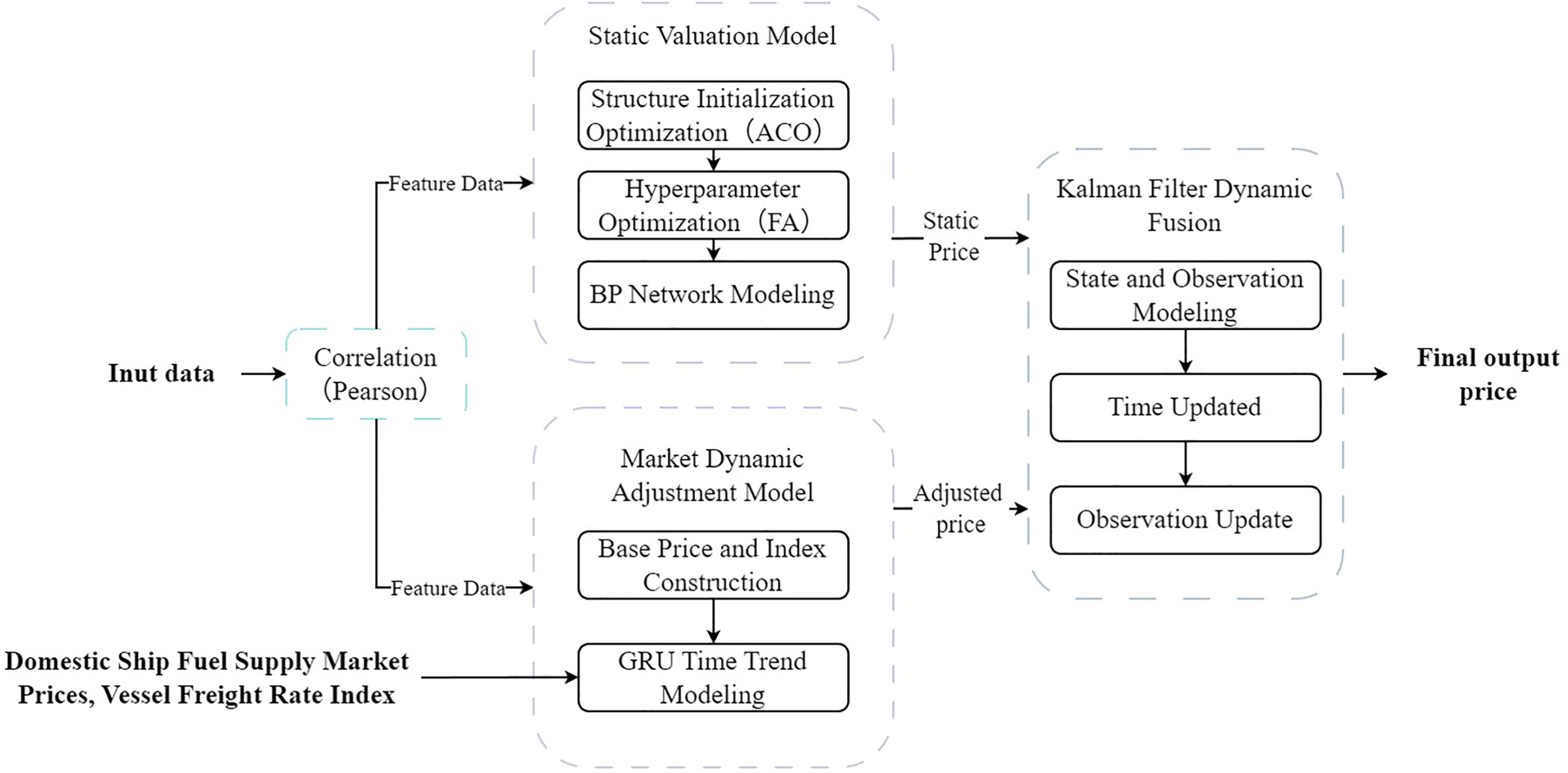
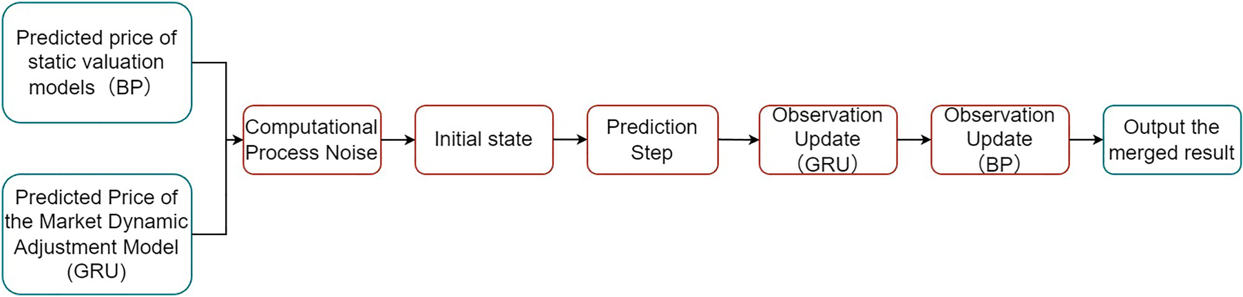
To enhance the accuracy and stability of ship price assessments, this paper proposes a used ship transaction price evaluation model that integrates static characteristics with dynamic time trends. The overall process, illustrated in Figure 1, comprises three components: the static valuation module, the dynamic market adjustment module, and the dynamic fusion module. Correlation Analysis of Secondhand Vessel Characteristics: To quantify the strength of association between secondhand vessel characteristics and transaction prices and identify key influencing factors, this study employs Pearson's correlation coefficient for correlation analysis. Static Valuation Module (ACO-FA-BP): This module proposes a BP neural network regression prediction model optimized by ACO-FA, aiming to enhance the stability and generalization capability of BP neural networks in predicting second-hand ship prices. Specifically, ACO optimizes the weight scaling factors across network layers to establish a robust initialization structure. FA then refines hyperparameters such as learning rate and weight decay on this foundation, thereby improving model convergence and generalization performance. This module outputs a benchmark price based on given static vessel characteristics, effectively evaluating the static value under “average market conditions.” Dynamic Market Adjustment Module (GRU): Based on historical transaction prices, a dimensionless price index is constructed. This price index is then combined with macroeconomic variables reflecting market conditions to form a multivariate time series. Specifically, a sliding time window is employed to use the price indices of six consecutive periods, national domestic ship-supplied fuel market prices, and the Yangtze River dry bulk shipping rate index as joint input features. The GRU neural network is then utilized to forecast future price indices, thereby capturing the dynamic impact of fuel costs and inland dry bulk shipping conditions on vessel prices over time. Dynamic Fusion Module (Kalman Filter): Within the state space framework, the Kalman filter linearly fuses the predicted values from the static model (BP benchmark price) with those from the dynamic market adjustment model (GRU price index-adjusted price). Based on the magnitude of observation errors and process errors at different stages, it dynamically adjusts the weights assigned to each in the final estimation, thereby achieving robust fusion of vessel prices.
Overall, this composite model can be understood as a layered structure comprising “static benchmark price assessment – market dynamic adjustment – information fusion”: the static module characterizes the impact of vessel-specific attributes on pricing, the dynamic module captures temporal evolution driven by macro variables such as oil prices and freight rates, while Kalman filtering integrates multi-source information through explicit linear weighting. For practical users, the benchmark price, market adjustment factors, and final valuation can be viewed separately.
Vessel characterization
The static characteristics of a ship reflect its inherent attributes and basic conditions, and these factors have a long-term and stable influence on the market value of a ship. This paper mainly selects the following indicators: Deadweight Tonnage (DWT): A key parameter reflecting a vessel's actual cargo-carrying capacity and operational scale. Generally, the higher the deadweight tonnage, the greater the vessel's cargo-carrying capability, and the higher its market value and profit potential. Vessel Age (VA): It indicates the number of years since the construction of the vessel was completed. The older the ship, the higher the maintenance cost, the lower the fuel efficiency, and the lower the market value. Horse Power (HP): reflects the performance of the ship's propulsion system, and the main engine power is directly related to the ship's speed, fuel consumption and oper-ating capacity. Dead Displancement (DD): a measure of the total weight of a ship in full load condi-tion. Gross Tonnage (GT): an indicator to measure the overall space volume of a ship, often used as a basis for port charges and tax accounting, and also has an important impact on the market value of the ship. Length, Breadth, Depth (L, B, D): these scale features together determine the design scale and loading space of the ship, which not only affects the seaworthiness and cargo capacity, but also indirectly affects the trading price. Length Overall (LOA): the horizontal distance between the foremost end of the bow and the last end of the stern of the hull (including the bow and stern raised decks) and superstructure of a ship.
The above static characteristics are relatively fixed and can reflect the basic technical level and design conditions of the ship, which are the basic factors for the formation of the trading price.
A framework for evaluating second-hand ship transaction prices based on static valuation and market dynamic adjustment using Kalman filter fusion.
In order to select the key static characteristics that have a significant impact on transaction prices, this paper adopts the Pearson Correlation Coefficient (PCC) to analyze the correlation of the main variables. Pearson Correlation Coefficient can measure the degree of linear correlation between two continuous variables, the range of values is, where 1 means completely positive correlation, −1 means completely negative correlation, 0 means no linear correlation. Its mathematical expression is as follows:
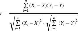
Where
In the task of ship price prediction, this paper employs a BP neural network as the core predictive model. To enhance the training stability and generalization capability of the BP neural network, this paper proposes an ACO–FA-based initialization and hyperparameter optimization method. The core approach involves: first, utilizing the Ant Colony Optimization (ACO) algorithm to optimize the initial layer scaling factor within a low-dimensional controllable space, thereby constructing a more robust initialization structure; then, based on this structure, fixing the initialization parameters and employing the Firefly Algorithm (FA) to optimize hyperparameters such as the learning rate and weight decay. This two-stage joint optimization improves both the network initialization and training process, ultimately enhancing the model's convergence and generalization performance.
BP neural network model
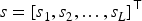
Let the input feature vector be

Where
Under the fixed BP network architecture and basic training framework, this paper further combines the Ant Colony Optimization (ACO) and Firefly Algorithm (FA) to jointly optimize the network's “initial structure” and “training hyperparameters.” The overall strategy comprises two phases: Phase 1 employs ACO to search for the scaling factors of weights across layers, enabling the construction of more optimal initial network parameters. Phase 2, building upon the fixed scaling, utilizes FA to search for scaling factors of learning rate and weight decay, thereby finely tuning the training process.
First, denote the parameter vector obtained through Xavier initialization as
Given s, multiplying the weights of the lth linear layer by a scale factor
This process maps different segments of
In the first phase, the ACO performs global optimization within the continuous search space
The ant colony algorithm iteratively searches for solutions under this objective through pheromone updates and a candidate solution generation mechanism based on Gaussian perturbations. It progressively converges toward regions with lower MSE, ultimately yielding the optimal scale factor
In the second stage, this paper introduces scaling vector
Where
The Firefly Algorithm performs swarm search on
After completing the above two stages, integrate
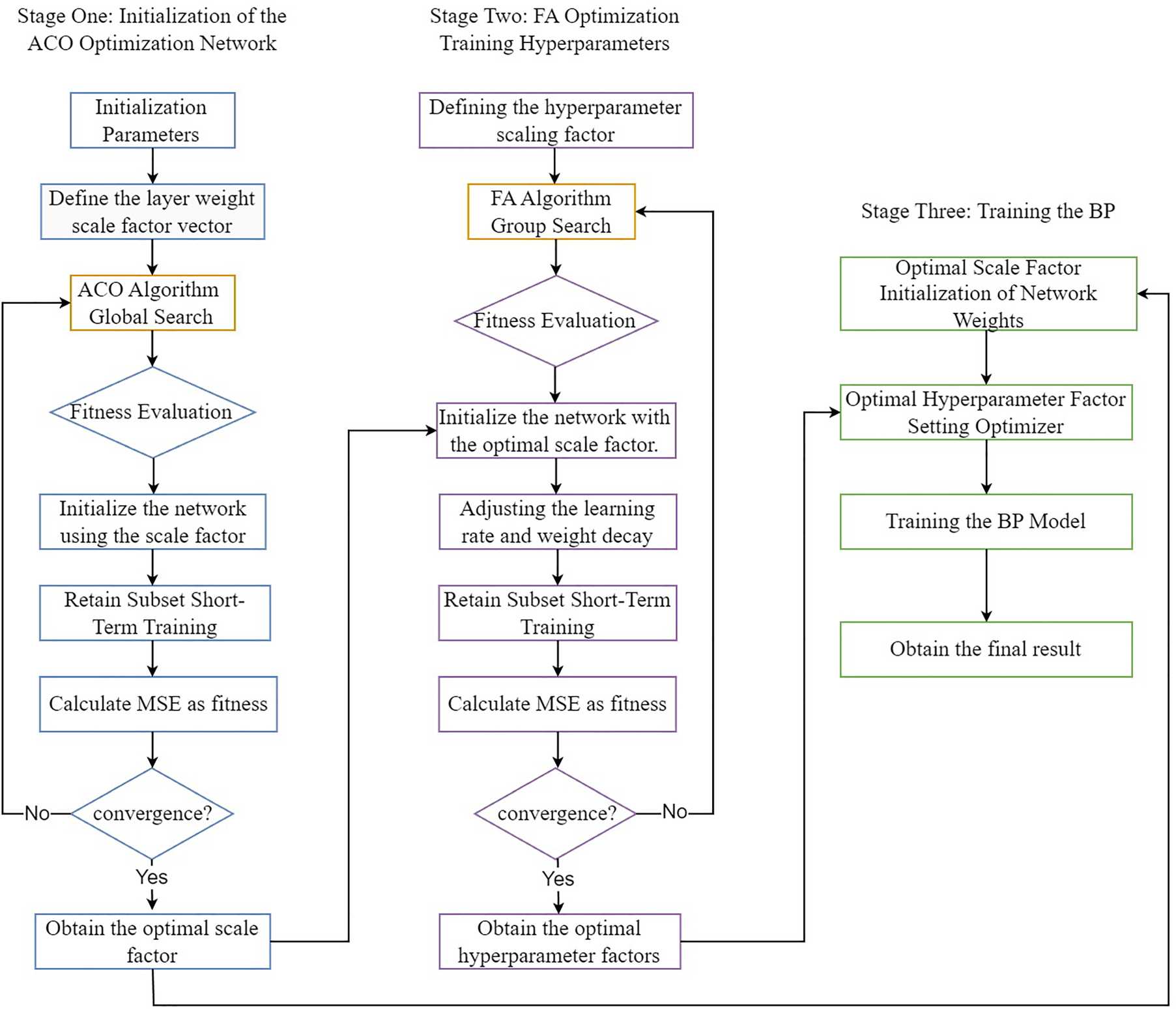
Flowchart of the ACO-FA two-stage optimization strategy.
Algorithm Pseudocode:
Algorithm 1 ACO–FA based training procedure for the BP neural network
Step 1: Data preprocessing & initialization Normalize input/output variables. Split data into training/validation (optionally keep a small hold-out subset). Define BP network architecture. Initialize weights (e.g., Xavier or small random values).
Step 2: Stage 1 — ACO for initialization scaling Encode each ant as a vector of layer-wise scaling factors (or neuron counts). For each ant: Apply its scaling to initialize the network. Perform short warm-up training on the hold-out/train subset. Compute validation MSE as fitness. Update pheromones based on fitness; generate new ants via pheromone-guided sampling. Repeat until convergence or iteration limit. Select the best ant as the ACO-optimized initialization.
Step 3: Stage 2 — FA for hyperparameters Define search ranges for learning rate, weight decay, etc. Encode each firefly as a hyperparameter vector. For each firefly: Train the network (using ACO initialization) for a few epochs. Compute validation MSE as brightness. Update fireflies via FA movement rules toward brighter ones. Repeat until convergence or iteration limit. Select the best firefly as the FA-optimized hyperparameters.
Step 4: Final model training Fix initialization (from ACO) and hyperparameters (from FA). Train the BP network on the full training set with early stopping. Save the final BP model for static valuation.
In ship second-hand market research, transaction samples are sparse and limited in distribution, making it difficult to obtain historical transaction data for second-hand vessels with fully consistent characteristics. This results in missing values in the time series, rendering it unsuitable for direct use in deep learning modeling. To address this, we first calculate a benchmark price for vessels, then construct a price index for the vessels. Finally, we employ a Gated Recurrent Unit (GRU) to model a multivariate sequence comprising this price index, national domestic vessel fuel supply market prices, and the Yangtze River dry bulk shipping rate index.
Price index construction
To eliminate the impact of individual vessel characteristics on transaction prices, this paper constructs a benchmark price based on historical transaction samples and calculates a dimensionless price index. Let the actual transaction price of the i-th transaction be

Among these,

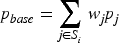
The benchmark price for Transaction i is the weighted average of comparable transaction prices:
Ultimately, the price index for Transaction i is:

By constructing this index, the influence of individual characteristics can be stripped away, transforming the original price sequence into a relative price sequence fluctuating around 1. This provides a smoother target variable for subsequent time series forecasting, with the specific process illustrated in Figure 3.
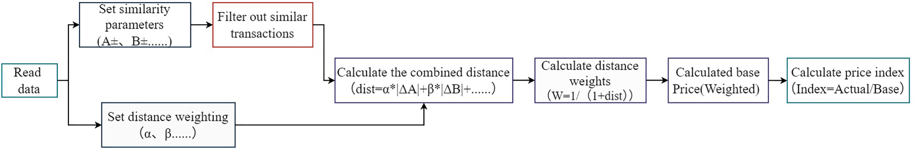
Flowchart for establishing benchmark prices and price indices.
After obtaining the price index series and corresponding benchmark prices, this paper employs a Gated Recurrent Unit (GRU) to construct a market dynamic adjustment model. With future price indices as the prediction target, historical price indices are combined with national domestic ship supply oil market prices and the Yangtze River dry bulk shipping freight rate index to form multivariate input features. The GRU predicts the next period's price index, which is then reconstructed into actual vessel transaction prices by integrating the corresponding benchmark prices. Sequence Sample Construction
To capture the dynamic characteristics of price indices, this paper employs a sliding time window to construct supervised learning samples. Let the time window length be L. For each time point t, the input vector

Among these, input vector
The corresponding prediction target is the price index for the next period. During sample construction, only historical data is used as input to prevent “information leakage” and ensure that the prediction pertains to future values. Sample pairs from all time points form the training and validation sets for model training and parameter tuning; a separate set of later samples serves as the test set to evaluate the model's external prediction capability. GRU Model
GRU is a commonly used recurrent neural network architecture that controls the retention and forgetting of historical information through update and reset gates, making it suitable for processing time-dependent sequential data. For input sequence
This paper employs a two-layer GRU architecture: the first layer receives multivariate time series inputs of length L (each period containing features such as price indices, national domestic ship supply oil market prices, and Yangtze River dry bulk shipping rates), outputting a sequence of hidden states. The second layer further processes these hidden states, outputting the hidden state at the final time step. Subsequently, a fully connected (Dense) layer maps the hidden state to a scalar prediction value:

Here, f denotes the nonlinear mapping of the fully connected layer, and W represents the network parameters. Model Training and Price Restoration
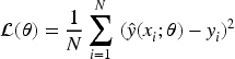
During the training phase, model parameters are optimized by minimizing loss functions such as MSE or Huber:
Here,
After obtaining the price index forecast value, restore the forecast price using the following formula:
Through the “index forecasting—price restoration” framework, the model isolates individual vessel characteristics while incorporating macroeconomic variables such as fuel prices and freight rate indices during the index forecasting stage. It ultimately restores the original price, thereby enabling time-series forecasting of vessel transaction prices.
Algorithm Pseudocode:
Algorithm 2 Training procedure for the price index and GRU-based market dynamic adjustment model
Step 1: Constructing the Base Price and Price Index For each historical transaction, identify comparable ships using key static attributes (e.g., DWT, age, engine power). Compute a base price as a weighted average of comparable ship prices. Define the dimensionless price index as the ratio of the actual transaction price to its base price. Collect the resulting price index series to represent market-level deviations from static valuation.
Step 2: Dynamic Feature Construction with Market Variables Align the price index series with external market variables, including domestic bunker fuel prices (coastal/inland) and the Yangtze River dry bulk freight index. For each time step, construct a feature vector consisting of the price index, fuel price, and freight index.
Step 3: Sequence Sample Generation Select a fixed window length L (e.g., 6 periods). For each time step ttt where a full window is available: Use the past Lperiods of features as the input sequence; Use the price index at t + 1 as the prediction target. Ensure that only past information is used to avoid information leakage. Split the samples chronologically into training, validation, and test sets.
Step 4: Data Preprocessing Handle missing values and outliers if necessary. Fit a standardization transform (e.g., StandardScaler) on the training features. Apply the same transform to the validation and test sets for consistency.
Step 5: GRU Model Construction (Market Dynamic Adjustment Model) Define a GRU-based neural network that accepts sequences of multi-dimensional features. Stack one or more GRU layers followed by fully connected layers, ending with a single output neuron for the next-period price index. Specify the loss function (e.g., MSE or Huber) and optimizer (e.g., Adam).
Step 6: GRU Model Training and Selection Train the GRU model on the training set and monitor validation performance. Apply early stopping and learning rate scheduling, saving the parameters that yield the best validation loss. Evaluate the trained model on the test set using metrics such as MAE, RMSE, and R2.
Step 7: Price Reconstruction and Dynamic Adjustment Interpretation Use the trained GRU to predict next-period price indices for validation and test samples. Multiply each predicted price index by its corresponding base price to obtain dynamically adjusted ship prices. Interpret the GRU output as the market dynamic adjustment term, capturing the joint influence of historical price indices, fuel prices, and freight indices.
To simultaneously utilize the prediction results of GRU and BP neural networks for ship price forecasting, this paper employs Kalman filtering to dynamically fuse the predictions from both models. State and Observation Modeling
Let the true price of period t be
Among these, Initial Value Setting
In the first phase, GRU and BP have provided initial prediction values
Here, Kalman Filter Recursive Fusion
Starting from the second iteration, each iteration of the Kalman filter process consists of two steps: the prediction step and the observation update.
First comes the prediction step. During this phase, the Kalman filter predicts the current state and covariance. Specifically, the current state is estimated as the previous iteration's state estimate

Next comes the observation update, which consists of two parts. First, the predictions from the GRU model are used to update the estimates, yielding the intermediate state estimate

Then, using the predictions from the BP model, the estimates are further updated to obtain the final fused state estimate

The Kalman gains
Kalman filter fusion flowchart.
This chapter will empirically evaluate the proposed Kalman filter framework that integrates static valuation with market dynamic adjustments using actual transaction data, comparing the performance of different models in ship price forecasting tasks. This includes an introduction to the dataset, an explanation of evaluation metrics, and a comparison of experimental results and analysis..
Data processing
Data sources
This study utilizes actual transaction data for secondhand dry bulk carriers in Chongqing, China, from 2020 to 2025. The dataset includes key indicators such as transaction value, deadweight tonnage, vessel age, transaction date, vessel dimensions, and main engine power. To ensure data quality and model stability, this study selected records of vessels under 20 years old and with deadweight tonnage below 8000 tons for analysis. After removing duplicate and outlier values, a total of 740 sample records remained. This screening criteria primarily aims to eliminate price distortions caused by excessively old vessels while avoiding the impact of extreme deadweight types on structural modeling. During the modeling process, the data was used in phases for different tasks. Data from 2020 to 2024 was employed for training, while data from June 2024 to May 2025 served as an independent sample for the final performance evaluation of the integrated model.
Data cleaning
Before constructing the neural network prediction model, this paper normalizes the original data, group aggregation and outlier processing to improve the data quality and consistency, and enhance the model learning effect and prediction performance. For the second-hand transaction data of inland dry bulk carriers in Chongqing (including deadweight tonnage, age, date and price), the transaction date is firstly standardized into “year and month” (YYYY-MM) format to realize the time dimension alignment; and then the data are grouped and aggregated according to the key indexes, and the average value of price is calculated to eliminate the redundancy and retain the first transaction id of each group as the index. The first transaction id of each group is retained as the index. In order to improve the robustness of the model, linear regression residual analysis is used to detect outliers: the model is built with ship parameters as features and transaction prices as dependent variables, and the standardized residuals (z-score) are calculated to eliminate 10 outliers with absolute values greater than 3, which effectively reduces the interference of extreme transactions and improves the generalization ability and prediction accuracy of the model.
Evaluation indicators
To quantify the model effect, the following three commonly used regressors are used in this paper:
MAE (Mean Absolute Error): a measure of the average of the absolute errors between the predicted and true values.
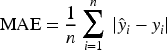
Where
RMSE (Root Mean Square Error): the square root of the mean of the squared error between the predicted value and the true value.
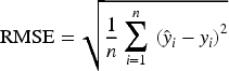
The RMSE is more sensitive to larger errors, so it can better reflect the performance of the model in dealing with extreme values. the smaller the RMSE is, the closer the model's prediction results are to the real values, and the better the model's performance.
R2 (coefficient of determination): a measure of the model's ability to explain variation in the data.
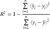
Where
A comprehensive evaluation of the above three metrics enables a holistic quantification of the model's predictive performance, providing a basis for model optimization and selection.
Before constructing the model, this paper first conducts an empirical analysis of the correlation between key variables and transaction prices to determine the strength of linear relationships among variables, thereby providing a basis for subsequent variable selection and modeling. Specifically, variables such as deadweight tonnage (DWT), vessel age (VA), and transaction time (year, month) from the sample data are selected for Pearson correlation analysis with transaction price (Price). The analysis results are as follows:
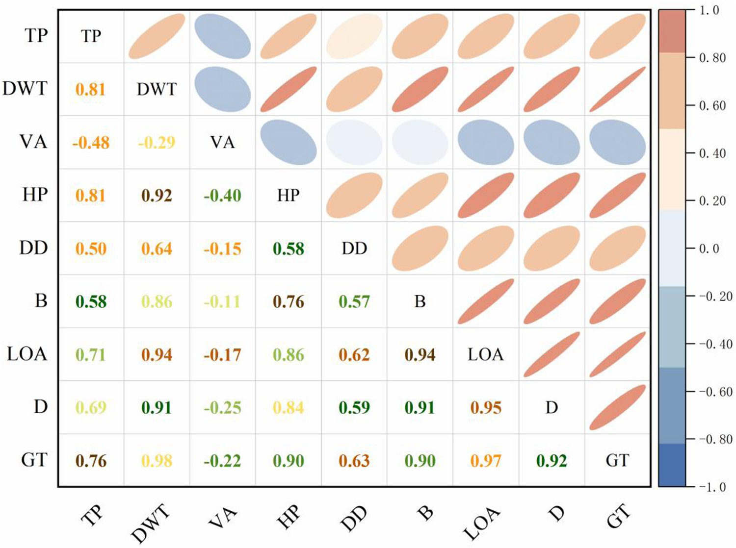
Correlation analysis between static structural parameters of used vessels and transaction amount.
As can be seen from the figure, Deadweight Tonnage (DWT) shows the strongest positive correlation (0.81) with Transaction Price (TP), while Vessel Age (VA) shows a significant negative correlation (−0.48) with price, indicating that the price of new vessels is generally higher than that of older vessels. Other variables such as Gross Tonnage (GT) and Length Overall (LOA), although also correlated with price, are prone to introduce redundant information due to high covariance with Net Tonnage (NT). Based on the above analysis, this paper finally selects Net Tonnage (NT) and Vessel Age (VA) as the main input features for both the static and dynamic modeling phases. This selection has clear economic interpretability and also helps to reduce model complexity and improve modeling stability.
Model and Hyperparameter Settings
This paper employs a feedforward BP neural network for ship price prediction, with inputs being deadweight tonnage (DWT) and vessel age (VA), and the output being ship price (Price). The network architecture consists of a two-layer hidden multilayer perceptron, with 128 neurons per layer and an ELU activation function, and a single linear neuron in the output layer. Weights are initialized using Xavier uniform initialization. Training employs the AdamW optimizer (learning rate 0.001, weight decay 0.0001) with a batch size of 32 and a maximum training epoch of 200. The loss function is mean squared error (MSE). Model optimization is divided into two parts: First, the Ant Colony Optimization (ACO) algorithm is used to optimize the weight scaling factor for each layer within the range of 0.5–2.0, with a population size of 30 and a maximum of 30 iterations. Second, the learning rate and weight decay scaling factors are optimized using the Firefly Algorithm (FA) within ranges of 0.5–3.0 and 0.3–3.0, respectively, with a population size of 30 and maximum evolution generations of 30. Prediction error serves as the evaluation criterion for both. Cross-Validation and Ablation Experiment Design
To comprehensively evaluate the effectiveness of the initialization search strategy, this paper employs a “5 random seeds × 5-fold cross-validation” design, taking the average of each fold's results as the comprehensive metric. The comparative experiments for the three training schemes are as follows: ① Baseline-BP: Standard BP training with Xavier initialization and fixed AdamW hyperparameters; ② ACO-init: Incorporates ACO prior to training to optimize only the weight scale of each layer, with hyperparameters consistent with the baseline; ③ ACO-FA: Adds FA to ACO-init to optimize the scaling factors for learning rate and weight decay. Experimental results are shown in Figure 6, where the RMSE of all three models progressively decreases: Baseline-BP yields a median value of approximately 58.96, ACO-init reduces it to 58.45, and ACO-FA further lowers it to 58.22, with overall error significantly reduced. The scatter plot indicates that in most cases, ACO-FA exhibits lower error than the other two schemes, validating the stable improvement in prediction accuracy achieved through joint optimization.
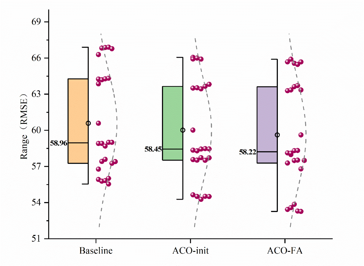
RMSE performance comparison of Baseline-BP, ACO-init, and ACO-FA.
Under the comprehensive results of multi-random seed (5 seeds) × 5-fold cross-validation, the prediction accuracy of the three training strategies is shown in Table 1. The overall average metrics for Baseline-BP are RMSE = 60.58, MAE = 40.23, R2 = 0.762. Under the ACO-init scheme, which only incorporates the ant colony optimization layer scale, the average RMSE decreased to 60.01, MAE decreased to 39.54, and R2 improved to 0.766. The ACO–FA scheme, which further combines the Firefly Algorithm to jointly optimize the learning rate and weight decay scaling factor, achieved optimal performance. The average RMSE was further reduced to 59.62, MAE decreased to 39.27, and R2 improved to 0.775. Statistical tests revealed that both meta-heuristic optimization methods (ACO-init and ACO-FA) significantly outperformed the baseline method in RMSE, MAE, and R2 (all pairwise comparisons, p < 0.05). Furthermore, Friedman tests confirmed highly significant overall differences among the three methods across all evaluation metrics (p < 0.05).
Performance comparison results and significance tests.
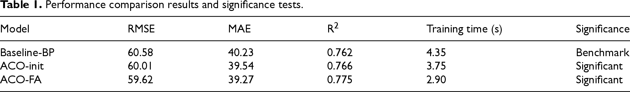
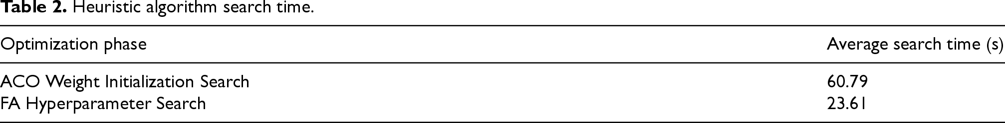
Beyond performance gains, our approach also improves training efficiency. As shown in Table 1, ACO-init and ACO-FA reduced training time by 13.8% and 33.3%, respectively, compared to Baseline-BP. This training acceleration stems from the meta-heuristic algorithm identifying superior initializations and hyperparameter configurations, enabling the network to converge more rapidly. Table 2 details the time expenditures for the ACO and FA search phases—one-time costs that yield sustained benefits throughout subsequent training once optimized configurations are obtained. Independent Sample Prediction
Heuristic algorithm search time.
This paper further constructs the final prediction model on the complete training dataset, splits it into training and validation sets at a 9:1 ratio, and evaluates its generalization performance on independent samples.
Figure 7 shows the fitness convergence curves for ACO and FA. Both swarm-based optimization methods reduced the target RMSE from approximately 192 to 190 and from 170 to 169 within the first few iterations, respectively, before rapidly stabilizing. Subsequent iterations fluctuated near the optimal values, indicating fast convergence speed and manageable computational overhead. On an independent test set, the proposed ACO–FA-optimized BP neural network maintains strong generalization performance on both the validation and independent test sets. The validation set achieves an R2 of 0.791 (as shown in Figure 8), while the independent test set yields an RMSE of 49.64, MAE of 35.41, and with an R2 of 0.779. This demonstrates the model's ability to accurately capture the nonlinear relationship between shipping rates, DWT, and vessel age on unseen samples.
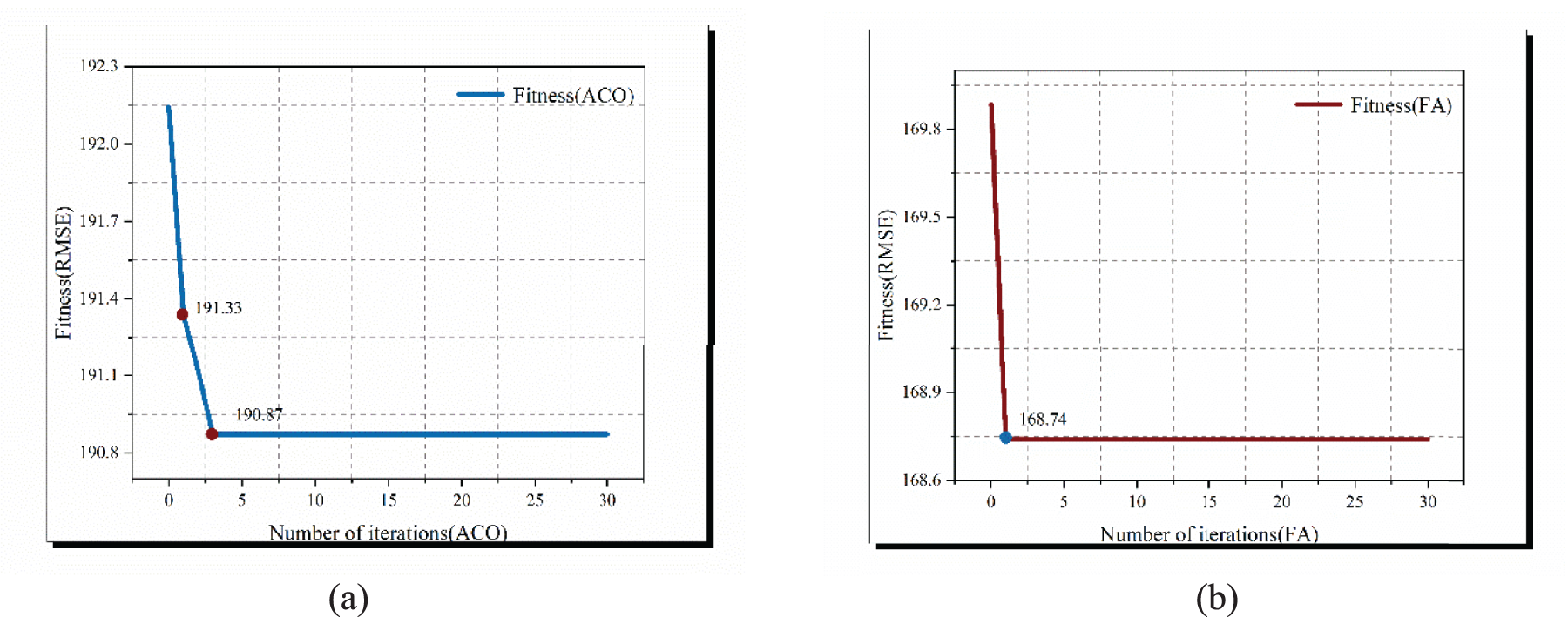
Adaptive iteration process of ACO and FA (RMSE). (a) ACO Fitness Iteration Process. (b) FA Fitness Iteration Process.
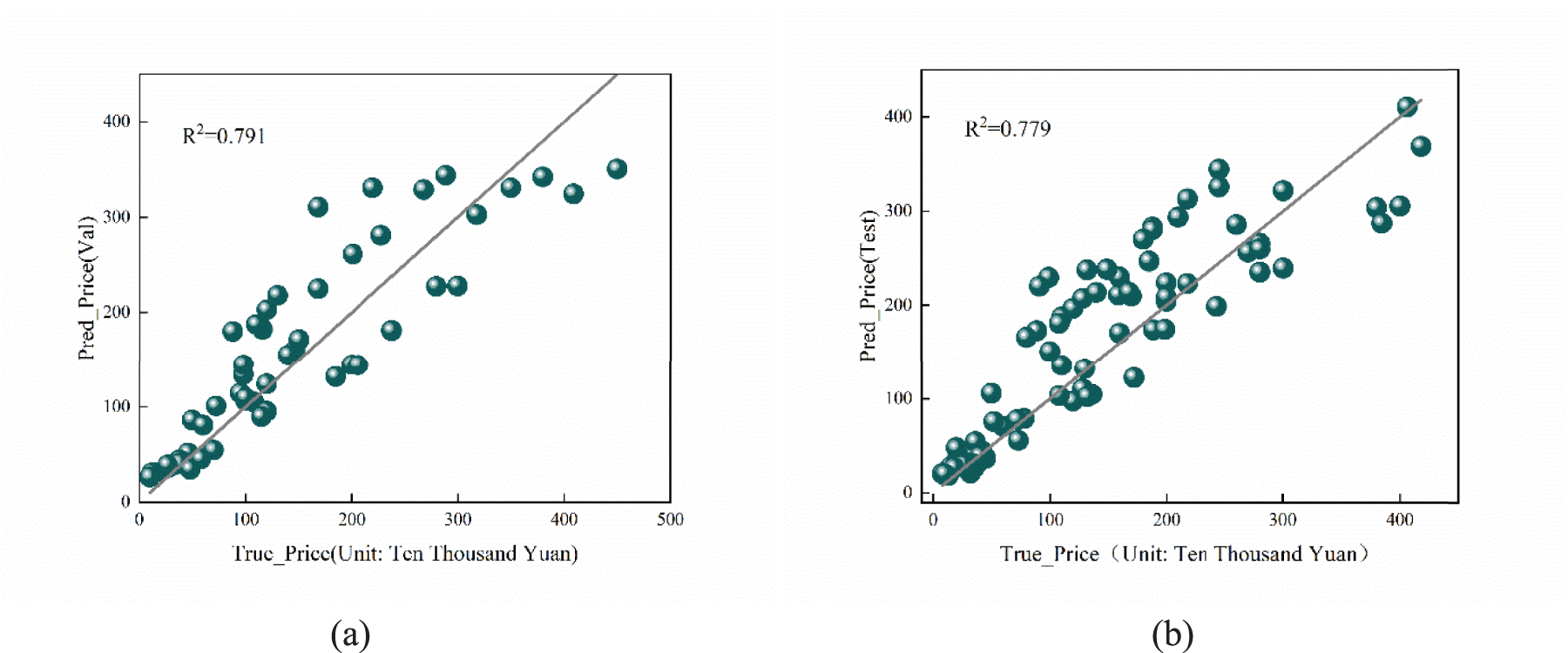
Fitting lines for the validation set and test set. (a) Val. (b) Test.
All experiments in this section are based on the benchmark prices and price indices constructed using the method described in Section 2.3.1. On this foundation, the data from 2022 to 2024 is divided into training and validation sets, while the data from 2024 to 2025 is allocated to the test set. Model Comparison
This paper first conducts a comparative evaluation of Gated Recurrent Unit (GRU), Long Short-Term Memory (LSTM), K-Nearest Neighbor (KNN) regression, and ARIMA models under the condition of using only the single variable of price indices. The four model types employ identical data partitioning and sample construction: time-ordered price index sequences are reconstructed using a sliding window of length 6, with the continuous 6-period indices serving as input and the next-period index as the prediction target. For the neural networks, GRU and LSTM employ identical structures and training settings: two recurrent layers (32 and 16 units, respectively), followed by a 32-dimensional ReLU fully connected layer and a one-dimensional linear output layer. The Huber loss function is used, with Adam as the optimizer set to a learning rate of 5 × 10⁻⁴ and a maximum training epoch of 300. KNN flattens the 6-period index window into a 6-dimensional feature and employs k = 5 k-nearest neighbor regression. ARIMA estimates an ARIMA(11,1) model on the training set price index sequence and performs dynamic forecasting for the corresponding periods in the validation and test sets.
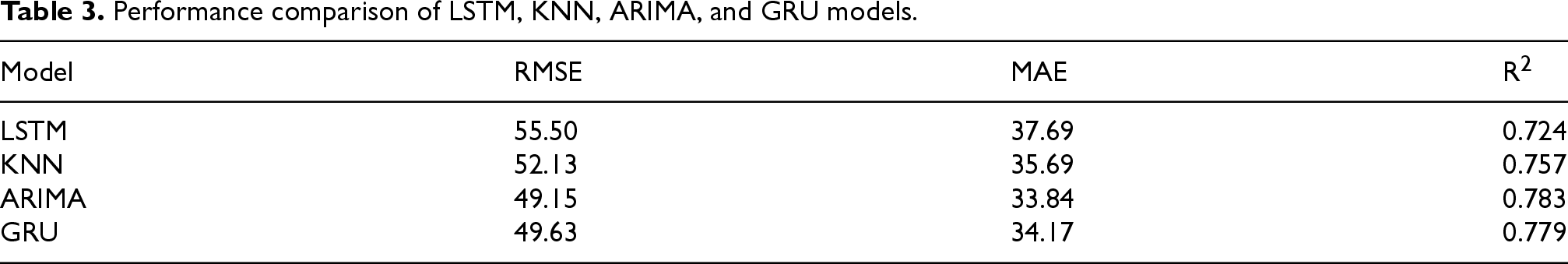
The comparative experimental results are shown in Table 3. Under the current sample size and feature settings, the out-of-sample forecasting performance of the four models on the price dimension is generally comparable. Among them, GRU and ARIMA perform relatively best and are very close to each other. Within the test set, GRU achieved a price prediction error of MAE = 34.17, RMSE = 49.63, and R2=0.779. ARIMA's RMSE and MAE were nearly identical to GRU's, while LSTM and KNN demonstrated slightly inferior overall performance. Based on paired t-tests of absolute price errors on the test set, the error advantages of GRU over ARIMA, LSTM, and KNN did not reach conventional significance levels. Considering overall accuracy, statistical test results, and the convenience of subsequently incorporating multi-source time series features such as oil prices and freight rates, this paper ultimately selects GRU as the primary method for the market dynamic adjustment model. Figure 9 presents a comparison of predicted prices versus actual prices across different models on the test set. Market Dynamic Adjustment Modeling and Results Analysis
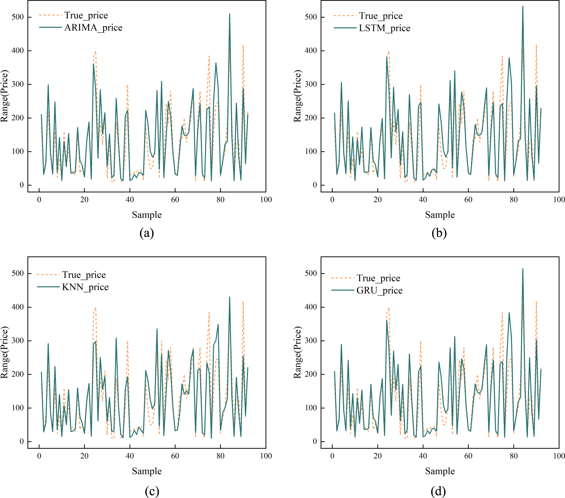
Comparison of ARIMA, LSTM, KNN, and GRU models with actual prices (price unit: ten thousand Yuan). (a) ARIMA. (b) LSTM. (c) KNN. (d) GRU.
Performance comparison of LSTM, KNN, ARIMA, and GRU models.
This paper introduces the national domestic ship fuel supply market price and the Yangtze River dry bulk shipping rate index based on the price index, constructing a multivariate time series forecasting framework. Specifically, a three-dimensional time series window of length 6 is formed by combining the price index, fuel price, and shipping rate index over six consecutive periods. The price index of the seventh period serves as the forecasting target, with feature standardization performed using StandardScaler on the development sample. K-fold cross-validation with rolling time windows is employed to optimize the GRU architecture and hyperparameters. By evaluating the validation set's price RMSE and R2 across different hidden layer sizes, dropout rates, and L2 regularization strengths, a compact configuration with strong generalization is selected: A two-layer GRU (first layer with 8 units outputting the full sequence, second layer with 4 units outputting the final hidden state), followed by an 8-dimensional ReLU fully connected layer and a one-dimensional linear output layer. Approximately 0.3 dropout and L2 regularization at the 10−3; magnitude were added to suppress overfitting. The training process employed the Huber loss function with an Adam optimizer set to a learning rate of 5 × 10⁻⁴. Based on these hyperparameters, the model was retrained on the entire development dataset.
As shown in Figure 10, both curves exhibit a monotonically decreasing trend with increasing iterations. They gradually stabilize after approximately 40 iterations, ultimately converging to similar levels around 0.10. Notably, the validation loss does not show any significant increase or noticeable divergence from the training loss. This indicates that under the current network architecture and regularization configuration, the model exhibits no significant overfitting during training, demonstrating strong fitting capability and generalization performance. On the independent test set, R2 reaches 0.779, while RMSE and MAE decrease to 49.64 and 33.09, respectively.
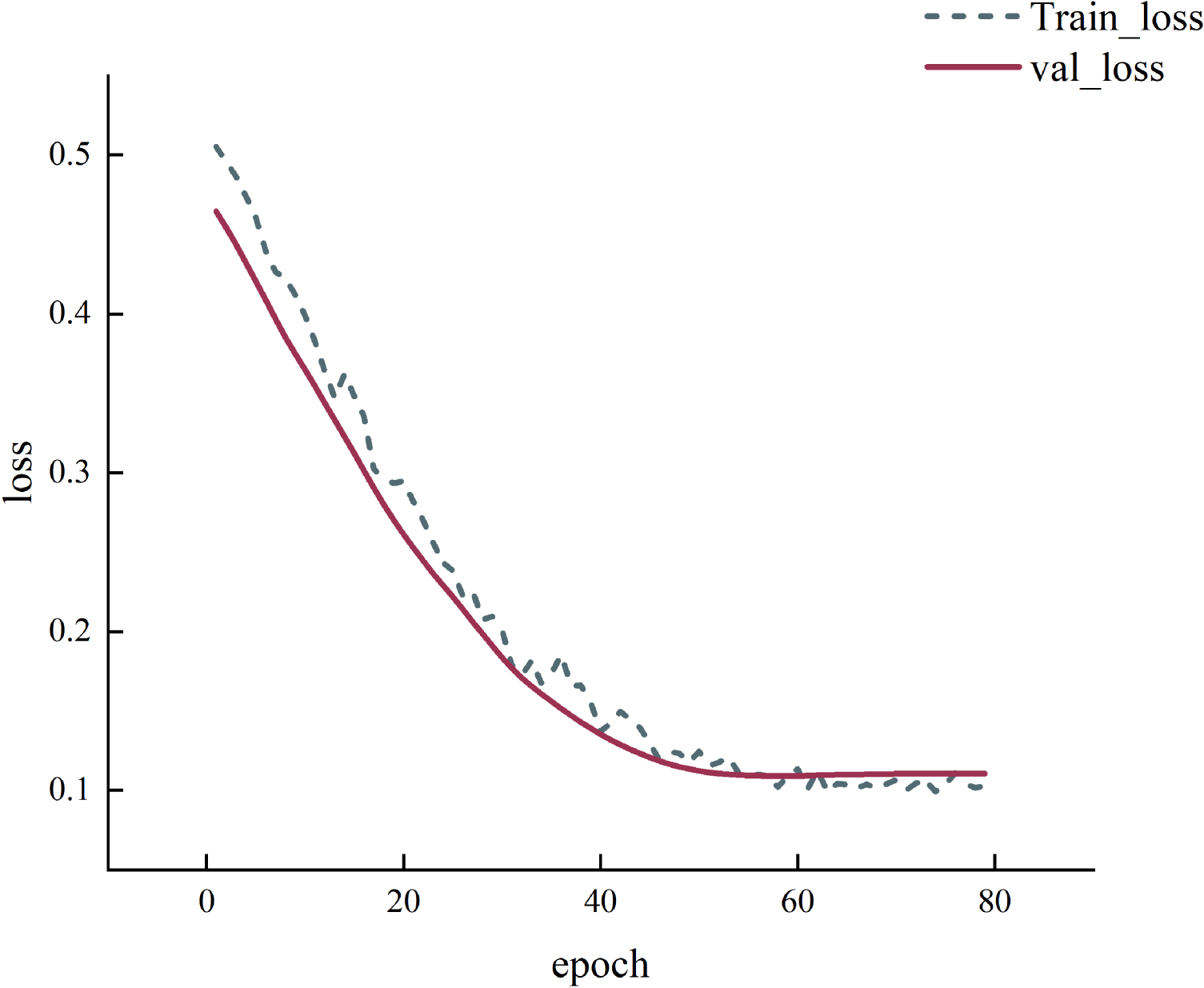
GRU model training and validation set loss curves over iterations.
In this experimental section, the ACO-FA-optimized BP neural network and GRU neural network were each trained on the same test dataset (used dry bulk carrier transaction records from May 2024 to May 2020) to generate two sets of price predictions. These predictions were then treated as two observations of the same true price and fed into the Kalman filter. The observation noise variance was taken as the variance of residuals (
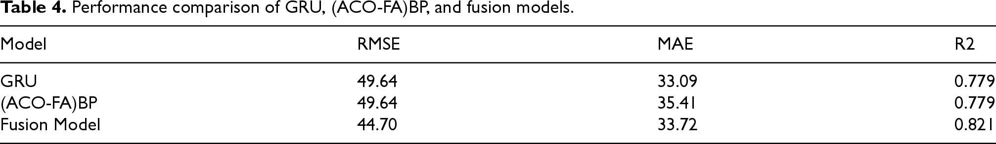
After integrating the two models using Kalman filtering, the overall model performance improved further, as shown in Table 4: The MAE of the integrated model decreased to 33.72, the RMSE significantly dropped to 44.70, and the R2 increased to 0.821. Compared to the BP model optimized by ACO-FA alone, the fusion model achieved approximately 4.8% lower MAE, 10.0% lower RMSE, and 5.4% higher R2; Compared to the standalone GRU model, the MAE of the fusion model remained essentially unchanged at 33.09, while RMSE decreased by approximately 10.0% and R2 increased by approximately 5.4%. Overall, this demonstrates that the fusion of static (BP) and dynamic (GRU) features based on Kalman filtering effectively leverages the complementary strengths of both types of information. Without altering the original model structure, this approach significantly enhances the accuracy and stability of price forecasting.
Performance comparison of GRU, (ACO-FA)BP, and fusion models.
Performance comparison of GRU, (ACO-FA)BP, and fusion models.
To compare the performance of different models in predicting used ship prices, we conducted experiments using XGBoost, Random Forest, and LightGBM. Each model employed 1000 trees, a maximum depth of 5, a learning rate of 0.01, and the squared error loss function. The Random Forest model employed 1000 trees with a maximum depth of 5. All models were trained using default hyperparameters. The performance comparison results across different models are presented in Table 5.
Comparison of predictive performance across different models on an independent test set.
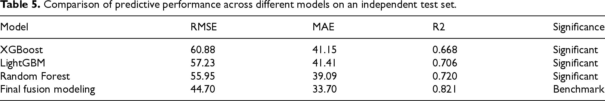
The Kalman Fusion model demonstrated the best overall performance among the three comparison models (as shown in Table 5): On the same test set, compared to XGBoost, Random Forest, and LightGBM, the fusion model reduced RMSE by approximately 20%–27%, decreased Mean Absolute Error (MAE) by roughly 14%–19%, while the corresponding R2 improved from approximately 0.67–0.72 to 0.821. This indicates that the ensemble model significantly outperforms single-model regression in both error magnitude and goodness-of-fit. Paired t-test results based on sample-level absolute errors show that under the one-tailed hypothesis test with the alternative hypothesis “comparison model error > fusion model error,” the p-values for all three comparison models are less than 0.05. This further validates the statistical significance of this advantage. Therefore, the Kalman fusion method demonstrates higher predictive accuracy and more stable fitting capabilities in price forecasting tasks. Figure 11 compares the Kalman filter-fused prices with actual transaction prices.
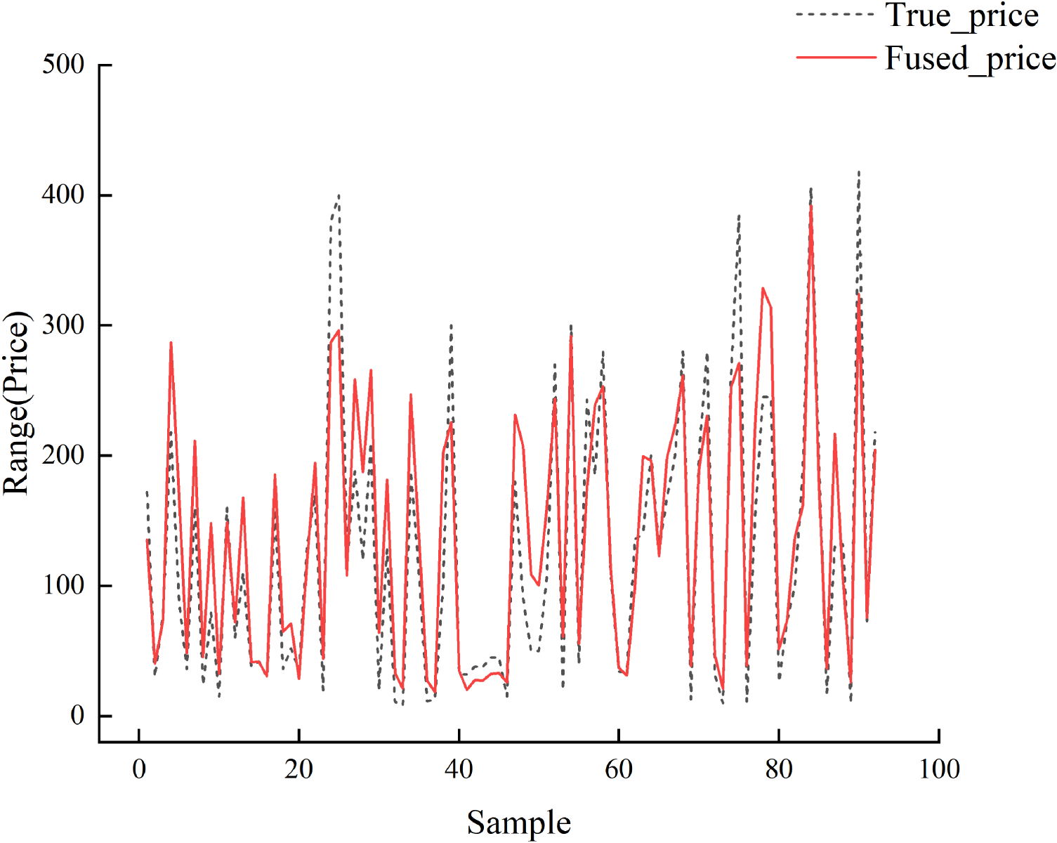
Comparison of Kalman filter fusion prices and actual transaction prices.
This paper addresses the challenge of predicting ship transaction prices by proposing a Kalman filter-based method that integrates static valuation with dynamic market adjustments for used vessels, achieving favorable results. The primary research contributions and conclusions are as follows: Kalman Filter-Based Fusion of Static Valuation and Market Dynamic Adjustment for Evaluating Transaction Prices of Used Inland Waterway Vessels: This paper constructs a fusion model integrating Kalman filter-based static valuation with market dynamic adjustment. It employs an ACO–FA-optimized BP neural network (static) and a GRU model (market dynamic) as dual observations of the same true price, achieving dynamic weighted fusion over periods without altering the underlying structures of the two base models. Experimental results demonstrate that compared to standalone GRU and (ACO–FA)BP models, the fusion model exhibits significantly reduced RMSE and MAE on the test set, with R2 improving to 0.821, indicating higher predictive accuracy and enhanced stability. Compared to traditional machine learning models such as XGBoost, Random Forest, and LightGBM, the fusion model also outperforms in terms of error and goodness-of-fit, with paired t-test results reaching statistical significance (p < 0.05). Overall, Kalman filtering effectively leveraged the complementarity between static structural features and dynamic temporal information, providing a more accurate and robust ensemble modeling approach for predicting second-hand ship prices. Static Valuation Module: A BP neural network model optimized by ACO-FA was constructed for ship price prediction. By introducing the Ant Colony Optimization (ACO) to optimize network initialization and the Firefly Algorithm (FA) to optimize training hyperparameters, the model's prediction accuracy was enhanced while reducing training time. Experimental results using 5-fold cross-validation demonstrate that the ACO–FA optimized model significantly outperforms the baseline BP model in metrics such as RMSE, MAE, and R2 while reducing training time by 33.3%. Statistical tests confirm the improvement in predictive accuracy is statistically significant. Thus, this static valuation model more accurately reflects the influence of vessel static attributes on price formation, providing ship buyers with robust and reliable static price assessment criteria. Market Dynamic Adjustment Module: A “Price Index–GRU” market dynamic adjustment model has been constructed. First, a dimensionless price index is constructed to mitigate the interference of individual characteristics on prices, thereby extracting price components that reflect market conditions. Subsequently, a sliding time window is employed to input multiple variable feature sequences—including the price index, national domestic ship fuel supply market prices, and the Yangtze River dry bulk shipping rate index—into the GRU model. The future period's price index serves as the prediction target. After forecasting, the results are combined with static valuation to form price levels with market dynamic characteristics. Empirical results indicate that under the current sample size and feature configuration, this GRU market dynamic adjustment model demonstrates robust predictive accuracy and stability. Its relatively simple structure and strong scalability assist investors in more clearly grasping the trends and outcomes of vessel price fluctuations in response to changing market conditions.
Future work can proceed in three directions: First, at the feature level, building upon existing variables such as price indices, fuel prices, and freight rate indices, incorporate richer macroeconomic and market variables including steel prices, interest rates, exchange rates, shipping capacity supply-demand indicators, and macroeconomic sentiment indices. Model these alongside individual vessel characteristics to enhance the ability to capture market volatility and cyclicality. Second, at the model level, building upon the ACO–FA optimization BP and GRU market dynamic adjustment models, introduce attention mechanisms, multi-source information fusion frameworks, or uncertainty quantification methods to improve the ability to capture price inflection points, risk intervals, and extreme scenarios, while maintaining interpretability; Third, at the application level, extend current methodologies to different vessel types, longer time horizons, and larger datasets. Systematically evaluate model robustness and practical utility through real-world valuation, investment, and pricing scenarios.
Footnotes
Acknowledgments
We extend our sincere gratitude to Professors Fu Daijun and Lu Yang of the Chongqing Shipping Exchange for providing the Chongqing vessel transaction data from 2020 to 2025. We also thank the Graduate Joint Training Base of China Shipbuilding Industry Corporation Southwest (Chongqing) Equipment Research Institute Co., Ltd for its financial support. We acknowledge the dedicated guidance of Professors Peng Zhongbo and Tong Liang from the research team, as well as the invaluable assistance, suggestions, and encouragement provided by students Zhao Jiawei, Ma Wen, Gou Rui, Tang Qianlong, and Zeng Fudong throughout the research process. Their support was crucial to the successful completion of this study.
Ethical approval and informed consent statements
Not applicable.
Author contributions
Liang Tong is primarily responsible for research conceptualization and methodology design, and for drafting the initial manuscript.
Yujie Guo is responsible for software implementation and result validation, and participates in manuscript revisions.
Daijun Fu and Yang Lu provided Chongqing's second-hand vessel transaction records and were responsible for the overall guidance and supervision of the manuscript, as well as project management.
Jiawei Zhao responsible for data organization and statistical analysis, and for creating charts and graphs.
Wen Ma is responsible for research and data collection, and assists with manuscript revisions.
Funding
The authors disclosed receipt of the following financial support for the research, authorship, and/or publication of this article: Funded by the Chongqing Jiaotong University-CSSC Southwest (Chongqing) Equipment Research Institute Co., Ltd Joint Graduate Student Training Base (JDLHPYJD2024008).
Declaration of conflicting interests
The authors declared no potential conflicts of interest with respect to the research, authorship, and/or publication of this article.
Data availability
The datasets generated and/or analyzed during the current study are not publicly available due to [reason, e.g., privacy restrictions, proprietary data] but are available from the corresponding author on reasonable request.