Building estimates for totals in respondent driven sampling

Abstract

Respondent-driven sampling (RDS) is a widely used methodology for estimating characteristics of hard-to-reach populations, such as homeless individuals, undocumented immigrants, and indigenous communities. Despite its effectiveness in obtaining representative samples, RDS lacks a robust estimation framework for total population figures. This limitation hinders its application in disaggregating Sustainable Development Goal (SDG) indicators, which are crucial for monitoring marginalized groups under the “leaving no one behind” principle of the 2030 Agenda. Building on previous research, we propose an improved estimator for total population counts based on the Generalized Weight Share Method (GWSM). Our approach employs a multi-phase sampling technique and ensures unbiased estimates when post-seed selections are random. Additionally, we introduce an approximation method for cases where some network information is unknown. We compare our method to traditional RDS estimators, highlighting its advantages and limitations. The paper is structured as follows: we first analyze RDS as an indirect sampling method, then extend our model to scenarios with partial link observations. We also address potential biases and present empirical analyses that validate our approach. Our findings contribute to refining RDS estimation techniques, enhancing its reliability for policy-relevant data collection.

Keywords

Indirect sampling GWSM estimator

1 Introduction

This paper focuses on respondent-driven sampling (RDS), an effective survey methodology for estimating characteristics of hidden populations, such as homeless individuals and undocumented immigrants, as well as hard-to-measure groups, like minorities and indigenous peoples.

The 2030 Agenda emphasizes the principle of “leaving no one behind.” However, many Sustainable Development Goal (SDG) indicators need to be more broadly accessible to the most marginalized and vulnerable populations. Currently, most SDG indicators lack the necessary level of disaggregation to effectively monitor the socioeconomic conditions of these groups. As a result, it is challenging to gather reliable structural data or to keep up with emerging phenomena that necessitate targeted, evidence-based policy actions.

RDS gathers information on these populations by leveraging relationships between their members. Its effectiveness increases when used alongside other information sources, such as administrative or geographical data. RDS is a network-based sampling technique^1,2 first developed by Heckathorn (1997,.³) Due to its viable sampling technique and reasonable inferential approaches, RDS has become the preferred method for sampling hard-to-reach populations. Since its inception, RDS has been used in numerous investigations worldwide.⁴

The research process begins with a small group of participants who are already known to the researchers. Each participant is given a few unique coupons to distribute, using a random method, to individuals in the larger population, inviting them to participate in the study. This process continues until the desired number of respondents is reached, which helps to expand and diversify the sample. While the selection of the initial participants is non-random, subsequent contacts are chosen at random. The process concludes when only previously identified individuals are encountered, or after reaching a predetermined data collection point, such as the fifth step.

Heckathorn (1997³) employed a Markov model to analyse the peer recruitment process, demonstrating that bias inherent in the initial convenience sample gradually diminished as the sample size increased over successive waves. He found that, irrespective of the initial sample or the chosen seeds, the process ultimately reached an equilibrium as it expanded. The conclusion drawn was that this sampling technique could yield reliable results, provided enough waves were conducted, indicating that any selection of seeds could ultimately lead to the same equilibrium sample composition. However, the paper did not clarify how to derive an unbiased estimate of totals.

The RDS method lacks a robust estimation methodology that can adapt to various conditions. While it is useful for estimating mean and proportion values, the accuracy of total estimates relies on unknown information regarding the total number of links. Additionally, it is affected by several factors, including the characteristics of the network that connects individuals within the population.⁵

In our paper, we build upon the findings of Falorsi et al. (2023⁶). We propose a straightforward estimator of totals based on the Generalized Weight Share Method (GWSM) developed by Lavallé in 2007.⁷ This estimator employs a multi-phase sampling approach. If the selection of sampling units after the initial seeds is done randomly, our proposed estimator will be unbiased. Most of the quantities needed for the estimation can be known by the researcher responsible for calculating the survey estimates, as long as they effectively organize the data collection process. Additionally, we discuss how to compute an approximate version of the estimator if some of these quantities are unknown. The RDS method is well established in the literature, with a comprehensive summary of significant works available in.⁶ In this paper, we introduce a slightly different approach from those previously developed. To maintain conciseness, we will reference only the most essential works that are crucial for understanding the fundamental aspects of our proposal.

The article is organized as follows: Section 2 explains the RDS search process when all unit links are observed and discusses how this can be interpreted as indirect sampling. Section 3 extends this discussion to scenarios where only a few links are randomly observed at each step. Section 4 addresses potential issues that could undermine the proposed approach. Section 5 presents a discussion of the empirical analyses, providing a solid basis for our conclusions. Finally, Section 6 offers the conclusions.

2 The RDS research path

We denote by U a target population where each element is related to some of the others by some kind of relationship. Our aim is to estimate the sum of a variable $Y$ in $U$

\begin{aligned} Y = \sum_{k \in U} y_{k}, \end{aligned}

where

y_{k}

is the value of the

Y

variable of the unit k.

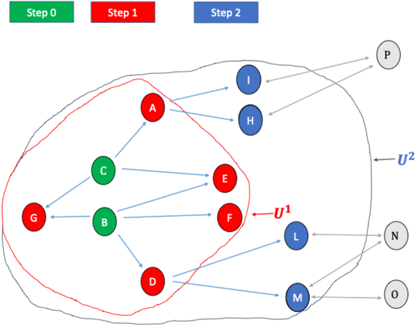
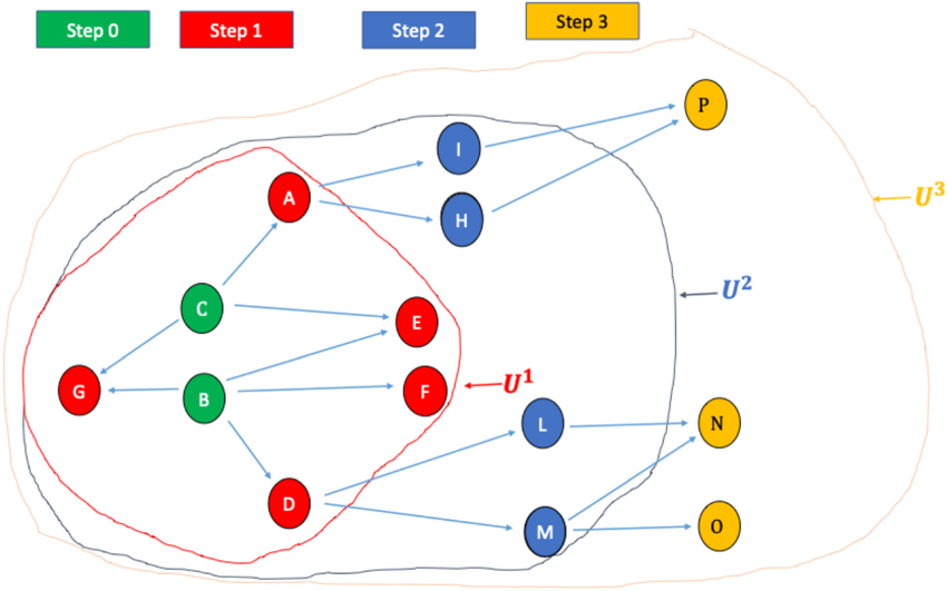
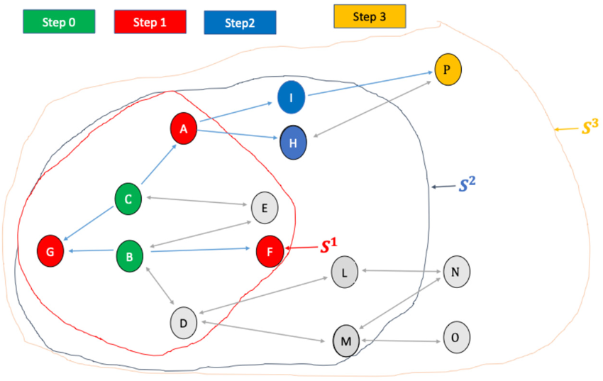
Let's use a specific example to illustrate how hand-induced notation can be applied to explore the RDS research method. To simplify the discussion, in the example, we assume that the value of each variable $y_{k}$ is always equal to 1. In this way, the total of the variable corresponds to the number N of elements in the population.

The accompanying Figure 1 displays a population of fourteen elements, labeled with the letters A through P from the Italian alphabet. These elements form a graph with bidirectional relationships, meaning that if Unit A knows Unit B, then Unit B also knows Unit A. The bidirectional relationships are represented by grey arrows in figure below pointing in both directions. The bidirectionality of the relationship implies that a unit cannot indicate as a link a unit with which the mutual relationship is weak, and that would not indicate the unit itself. Moreover, this property would limit the sizes and complexity of the networks.

Figure 1.

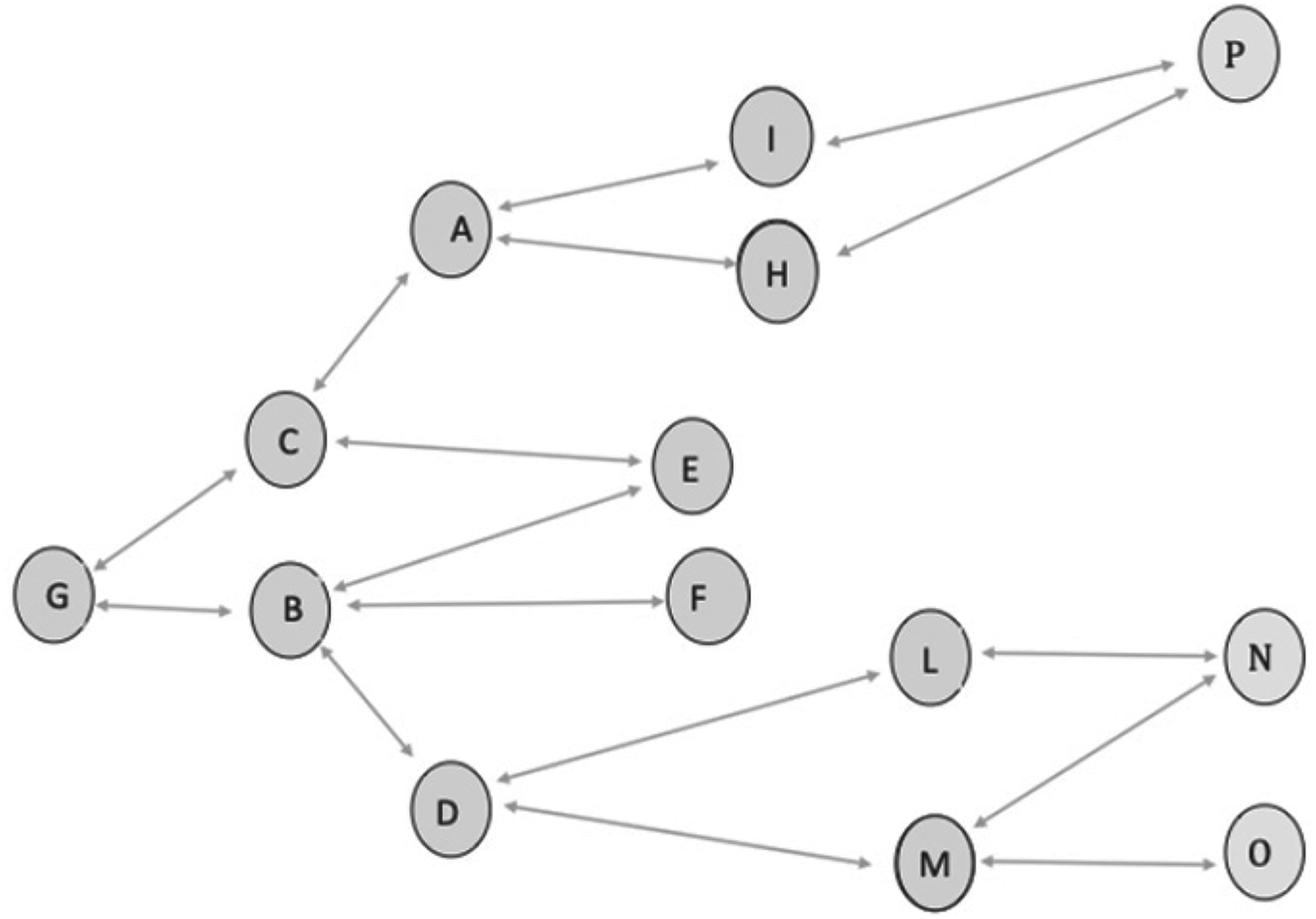
Population of the example.

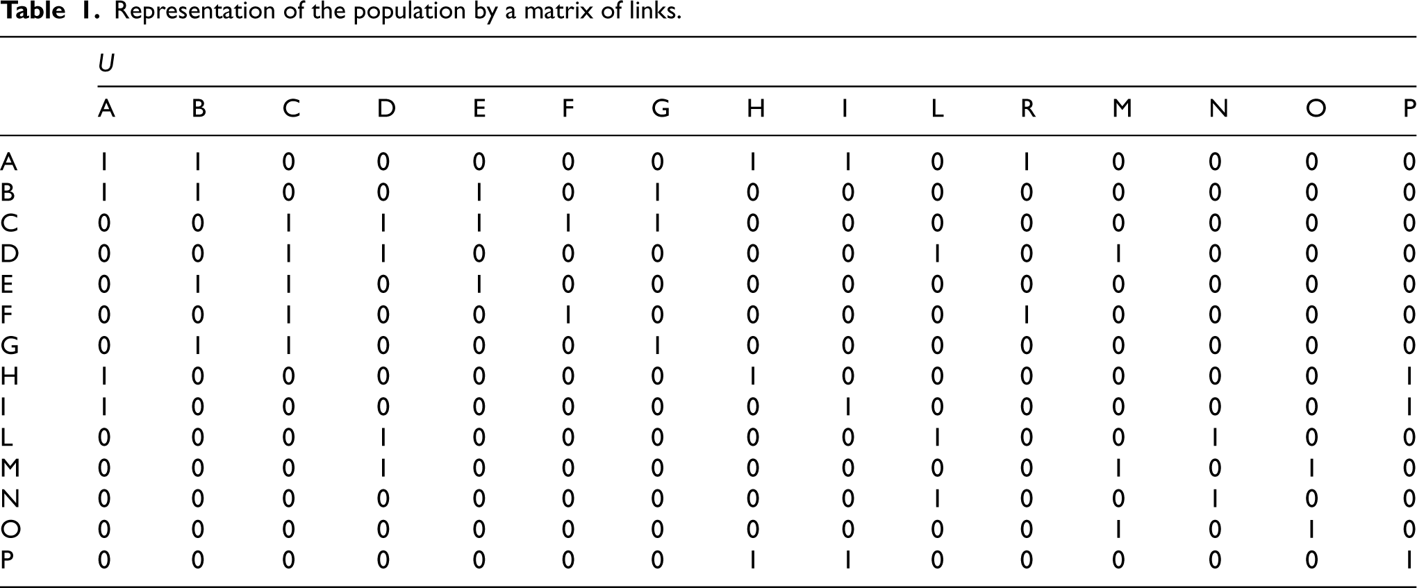
The latter population can be represented by a symmetric matrix of 0 s and 1 s, where 1 indicates a link between the units (see Table 1).

Table 1.

Representation of the population by a matrix of links.

	$U$
	A	B	C	D	E	F	G	H	I	L	R	M	N	O	P
A	1	1	0	0	0	0	0	1	1	0	1	0	0	0	0
B	1	1	0	0	1	0	1	0	0	0	0	0	0	0	0
C	0	0	1	1	1	1	1	0	0	0	0	0	0	0	0
D	0	0	1	1	0	0	0	0	0	1	0	1	0	0	0
E	0	1	1	0	1	0	0	0	0	0	0	0	0	0	0
F	0	0	1	0	0	1	0	0	0	0	1	0	0	0	0
G	0	1	1	0	0	0	1	0	0	0	0	0	0	0	0
H	1	0	0	0	0	0	0	1	0	0	0	0	0	0	1
I	1	0	0	0	0	0	0	0	1	0	0	0	0	0	1
L	0	0	0	1	0	0	0	0	0	1	0	0	1	0	0
M	0	0	0	1	0	0	0	0	0	0	0	1	0	1	0
N	0	0	0	0	0	0	0	0	0	1	0	0	1	0	0
O	0	0	0	0	0	0	0	0	0	0	0	1	0	1	0
P	0	0	0	0	0	0	0	1	1	0	0	0	0	0	1

RDS is developed through a series of successive search steps. In each step, after the initial one (referred to as step 0), links to the units listed in the previous step are chosen. Each search path ends when a unit that has already been selected is encountered. Once all search paths have come to an end, the RDS process is completed. Below, we will illustrate the RDS process step by step, assuming we observe all the units connected to those involved in the previous step.

2.1 Step 0

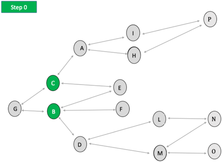
Step 0 involves selecting an initial sample ( $S^{0}$ ) from the target population. This selection process is non-random and relies on the researchers’ understanding and in-depth knowledge of the structure of the target population. In the example we are discussing, the initial sample $S^{0}$ includes units B and C, which are highlighted in green in Figure 2. In our notation, we denote values that depend on a specific RDS step with a superscript placed to the right of the corresponding quantity.

Figure 2.

Step 0 of the RDS process.

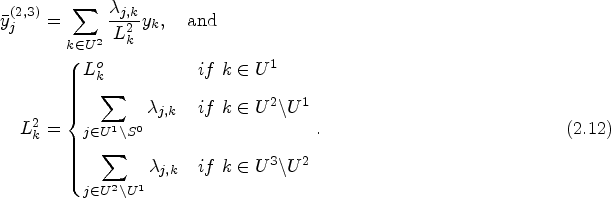
The total of the 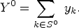$Y$ target variable defined at step 0 of the RDS process is denoted as $Y^{0},$ where

\begin{aligned} Y^{0} = \sum_{k \in S^{0}} y_{k} . \end{aligned}

In the example, we have

\begin{aligned} Y^{0} = y_{B} + y_{C} = 2. \end{aligned}

2.2 Step 1

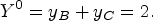
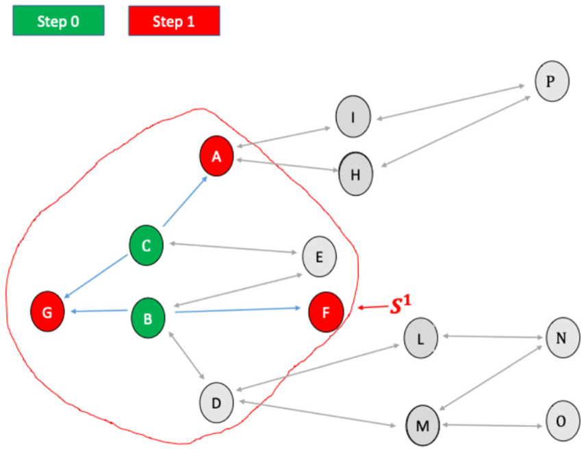
In Step 1, as shown in Figure 3, we observe $S^{0}$ and all the units linked to those in $S^{0}$ . Let $λ_{j, k}$ represent the link (0,1) variable, which is equal to one if Unit $j$ is connected to unit k, and zero otherwise, being $λ_{j, j} = 1$ . For each observed unit k, we gather information on the target variable $y_{k}$ and $L_{k} = \sum_{j \in U} λ_{j, k}$ , where the latter indicates the number of bidirectional links of unit k. The value of $L_{k}$ is obtained by asking Unit k. We individuate the Population set $U^{1} \equiv {k : λ_{j, k} = 1 | j \in S^{0}}$ , including all the units linked to those in $S^{0}$ . Since Unit $j \in S^{0}$ is linked with itself ( $λ_{j, j} = 1)$ , it is automatically included in $U^{1}$ , making $S^{0} \in U^{1}$ .

Figure 3.

Step 1 of the RDS process.

In the example, the units in $U^{1} \equiv {A, B, C, D, E, F, G,}$ are those highlighted in green and red in Figure 3.

Let $Y^{1}$ be the total of the variable $Y$ , captured by the RDS process up to step 1. In our example we have:

\begin{aligned} Y^{1} = \sum_{k \in U^{1}} y_{k} = y_{A} + y_{B} + y_{C} + y_{D} + y_{E} + y_{F} + y_{G} = 7. \end{aligned}

We can represent this situation as a specific case of indirect sampling,⁷ where the sample $S^{0}$ corresponds to the source population, and the population $U^{1}$ represents the target population. Using a standard result from this approach, the total for the population $U^{1}$ can be estimated as the sum of a variable constructed for each unit in $S^{0}$ . This variable is defined as the weighted sum of the variable $Y$ over all units in the target population ( $U^{1}$ ) that are linked to a unit in $S^{0}$ , with weights inversely proportional to the number of links pointing from the source population. Specifically, we can calculate $Y^{1}$ as:

\begin{aligned} Y^{1} = \sum_{j \in S^{0}} {\bar{y}}_{j}^{(0, 1)} \end{aligned}

(2.1)

where

\begin{aligned} {\bar{y}}_{j}^{(0, 1)} & = \sum_{k \in U^{1}} \frac{λ_{j, k}}{L_{k}^{0}} y_{k}, and \end{aligned}

(2.2)

\begin{aligned} L_{k}^{0} & = \sum_{j \in S^{0}} λ_{j, k} . \end{aligned}

(2.3)

Here, $L_{k}^{0}$ represents the number of links between unit k in the target population ( $U^{1}$ ) and the units in the source population ( $S^{0}$ ). In the superscript ${\bar{y}}_{j}^{(0, 1)}$ , the first digit indicates that Unit j was captured at Step 0, while the second digit represents that the value of the unit is computed considering all units captured up to Step 1 of RDS.

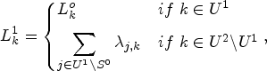
It is useful define $Y^{1}$ by using an incremental approach, as:

\begin{aligned} Y^{1} = Y^{0} + Y^{1 +}, \end{aligned}

(2.4)

where:

\begin{aligned} Y^{1 +} = \sum_{j \in S^{0}} {\bar{y}}_{j}^{(0, 1) +} \end{aligned}

(2.5)

is the incremental part of the total, being

\begin{aligned} {\bar{y}}_{j}^{(0, 1) +} = \sum_{k \in U^{1} ∖ S^{0}} \frac{λ_{j, k}}{L_{k}^{0}} y_{k} \end{aligned}

(2.6)

computed as

{\bar{y}}_{j}^{(0, 1)}

by excluding the units in

S^{0} .

The “+” symbol in the superscript of expressions 2.4, 2.5, and 2.6 indicates that the corresponding value is computed excluding the units from the source population, which in this case is

S^{0}

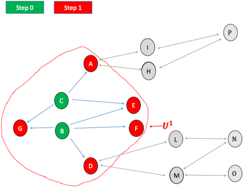
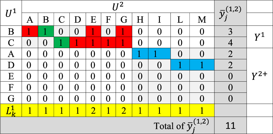
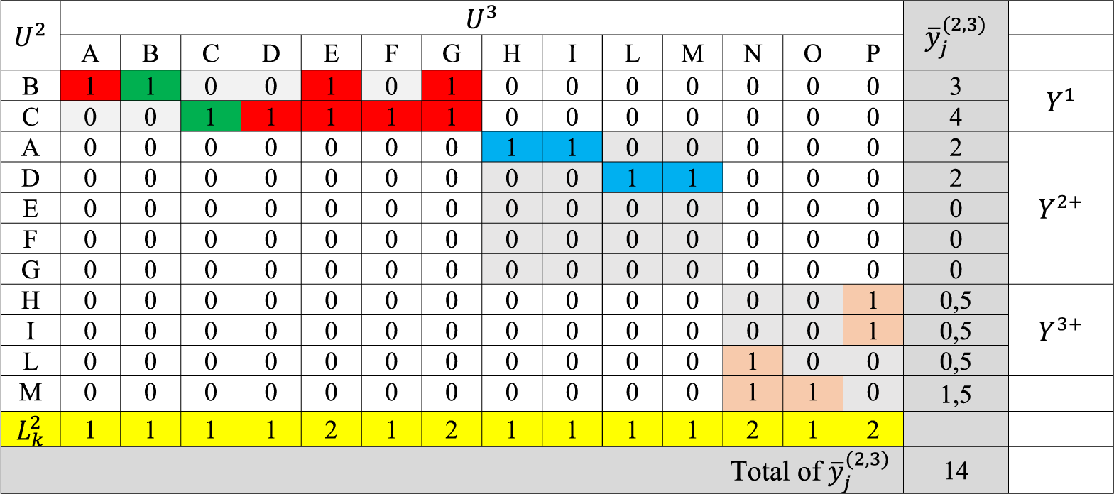
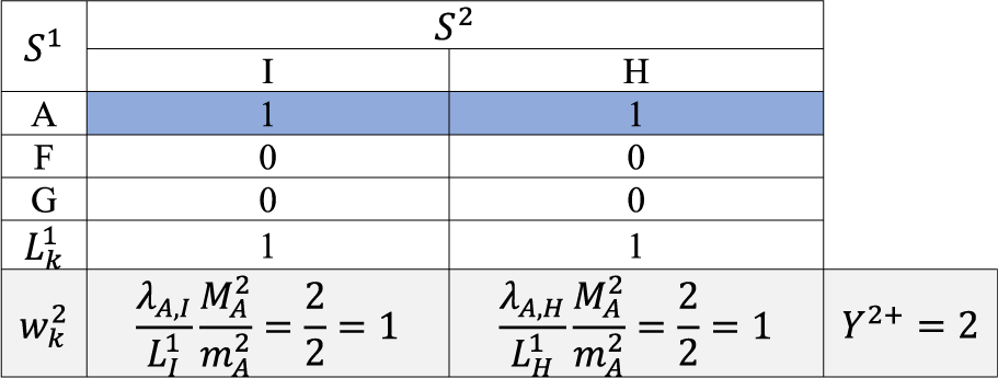
The indirect sampling formulation for writing the total may seem unnecessarily complex at first. However, it is essential because, it helps us address the issue of multiplicity, which arises when the same unit is detected through the connections of different units as seen below. To better understand the structure of the estimation method, it is helpful to introduce Table 2 that illustrates the relationships between the units selected in step 0 and those identified in step 1.

Table 2.

Example of the calculus of $Y^{1}$ via the indirect approach.

Proof of Formula 2.1. Proof of Formula 2.1.

Using a standard result from indirect sampling, with 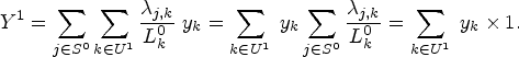$S^{0}$ as the starting population and $U^{1}$ as the target population, we can express $Y^{1}$ as:

\begin{aligned} Y^{1} = \sum_{j \in S^{0}} \sum_{k \in U^{1}} \frac{λ_{j, k}}{L_{k}^{0}} y_{k} = \sum_{k \in U^{1}} y_{k} \sum_{j \in S^{0}} \frac{λ_{j, k}}{L_{k}^{0}} = \sum_{k \in U^{1}} y_{k} \times 1. \end{aligned}

Proof of Formulae 2.4, 2.5 and 2.6. Proof of Formulae 2.4, 2.5 and 2.6.

Let 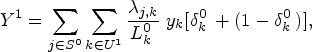$δ_{k}^{0}$ be a membership indicator variable that equals 1 if $k \in S^{0}$ , and 0 otherwise. We can reformulate $Y^{1}$ as

\begin{aligned} Y^{1} & = \sum_{j \in S^{0}} \sum_{k \in U^{1}} \frac{λ_{j, k}}{L_{k}^{0}} y_{k} [δ_{k}^{0} + (1 - δ_{k}^{0})], \end{aligned}

\begin{aligned} where Y^{0} & = \sum_{j \in S^{0}} \sum_{k \in U^{1}} \frac{λ_{j, k}}{L_{k}^{0}} y_{k} δ_{k}^{0} and \\ Y^{+} & = \sum_{j \in S^{0}} \sum_{k \in U^{1}} \frac{λ_{j, k}}{L_{k}^{0}} y_{k} (1 - δ_{k}^{0}) \; \end{aligned}

Comparing Figure 2 with Figure 3, we see that in this latter figure, the arrows starting from the

S_{0}

units have changed from bidirectional to one-way arrows highlighted with blue.

Let's continue the explanation from step 1 by noting that in the notation we've introduced and will continue to use for all subsequent steps, the units involved up to the second-to-last step (in our case, step 0) will always be identified by subscript j, while the units identified in the last step (in our case, step 1) will be denoted by subscript k.

2.3 Step 2

We observe $U^{1}$ , as shown in Figure 4, and all the links of their units. We individuate the set $U^{2} \equiv {k : λ_{j, k} = 1 | j \in U^{1}} .$

In our example, the units involved in $U^{2}$ are A, B, C, D, E, F, G, H, I, L, and M, where the units H, I, L, and M are those new.

We compute $Y^{2}$ as

\begin{aligned} Y^{2} & = \sum_{k \in U^{2}} y_{k} = y_{A} + y_{B} + y_{C} + y_{D} + y_{E} \\ + y_{F} + y_{G} + y_{H} + y_{I} + y_{L} + y_{M} = 11. \end{aligned}

In this case, $U^{1}$ represents the source population, whereas $U^{2}$ is the target population. When using the indirect search mechanism, adopting an incremental approach, we first have to build the matrix of links between $U^{1}$ and $U^{2}$ as a block diagonal matrix, where the links observed in the previous RDS step (those among units of $S^{0}$ and $U^{1}$ ) are in the first block. The second block includes the links among the units of $U^{1}$ and the new units of $U^{2}$ captured in the second RDS search Steps. This matrix is illustrated in Table 3.

Table 3.
Example of the calculus of $Y^{2}$ via the indirect approach.

On the basis of such a matrix, we have

\begin{aligned} L_{k}^{1} = {\begin{array}{ll} L_{k}^{o} & i f k \in U^{1} \\ \sum_{j \in U^{1} ∖ S^{0}} λ_{j, k} & i f k \in U^{2} ∖ U^{1} \end{array}, \end{aligned}

where

L_{k}^{1}

is obtained by summing the

λ_{j, k}

values rows of the column

k - th

of Table 3.

When computing the total $Y^{2}$ using the indirect approach, we have:

\begin{aligned} Y^{2} = \sum_{j \in U^{1}} {\bar{y}}_{j}^{(1, 2)} \end{aligned}

(2.7)

where

\begin{aligned} {\bar{y}}_{j}^{(1, 2)} = \sum_{k \in U^{2}} \frac{λ_{j, k}}{L_{k}^{1}} y_{k} . \end{aligned}

(2.8)

Adopting the incremental approach, we have

\begin{aligned} Y^{2} = Y^{1} + Y^{2 +} \end{aligned}

(2.9)

where:

\begin{aligned} Y^{2 +} = \sum_{j \in U^{1} ∖ S^{0}} {\bar{y}}_{j}^{(1, 2) +}, and {\bar{y}}_{j}^{(1, 2) +} = \sum_{k \in U^{2} ∖ U^{1}} \frac{λ_{j, k}}{L_{k}^{1}} y_{k} . \end{aligned}

(2.10)

2.4 Step 3

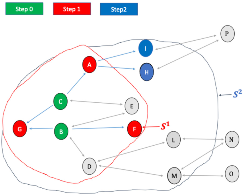
We observe $U^{2}$ , as shown in Figure 5, and all the links of their units, individuating the set

\begin{aligned} U^{3} \equiv {k : λ_{j, k} = 1 | j \in U^{2}} . \end{aligned}

Figure 4.

Step 2 of the RDS process.

In this case, $U^{2}$ represents the source population, whereas $U^{3}$ is the target population. We build the matrix of links between $U^{2}$ and $U^{3}$ by adding to the previous matrix (illustrated in Table 3) a third diagonal block which includes the links among the units of $U^{2}$ and the new units of $U^{3}$ . Taking an indirect approach to calculating the total $Y^{3}$ , we have:

\begin{aligned} Y^{3} = \sum_{j \in U^{2}} {\bar{y}}_{j}^{(2, 3)}, \end{aligned}

(2.11)

where

\begin{aligned} {\bar{y}}_{j}^{(2, 3)} & = \sum_{k \in U^{2}} \frac{λ_{j, k}}{L_{k}^{2}} y_{k}, and \\ L_{k}^{2} & = {\begin{array}{ll} L_{k}^{o} & i f k \in U^{1} \\ \sum_{j \in U^{1} ∖ S^{0}} λ_{j, k} & i f k \in U^{2} ∖ U^{1} \\ \sum_{j \in U^{2} ∖ U^{1}} λ_{j, k} & i f k \in U^{3} ∖ U^{2} \end{array} . \end{aligned}

(2.12)

Below is Table 4 for calculating $Y^{3}$ using the indirect method from the $U^{2}$ population.

Table 4.

Example of the calculus of $Y^{3}$ via the indirect approach.

Adopting the incremental approach, we have

\begin{aligned} Y^{3} = Y^{2} + Y^{3 +} \end{aligned}

(2.13)

where:

\begin{aligned} Y^{3 +} = \sum_{j \in U^{2} ∖ U^{1}} {\bar{y}}_{j}^{(2, 3) +} \; \; and\; \; {\bar{y}}_{j}^{(2, 3) +} = \sum_{k \in U^{3} ∖ U^{2}} \frac{λ_{j, k}}{L_{k}^{2}} y_{k} . \end{aligned}

(2.14)

2.5 Closing

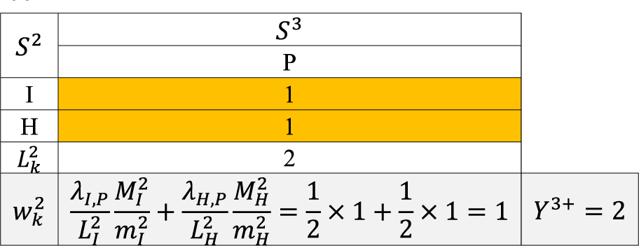
When restarting the RDS process, one notices that all the links of the N, O, and P Units have already been listed in previous steps. Hence, the RDS process closes, and the total of the cluster coincides with $Y^{3} .$ This latter is the total of all units connected directly or indirectly to those of initial sample $S^{0} .$

2.6 Caveat

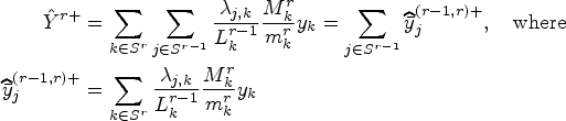
Before concluding this section, it is important to emphasize the relationship between the total network defined at the end of the RDS process and the actual total of the variable of interest. Consider the example illustrated in Figure 6, where the population is divided into three clusters: α, β, and γ. The total variable of $Y$ is the sum of the totals from these three clusters. If the initial sample $S^{0}$ includes only units from clusters α and β, the total computed at the end of the RDS process will reflect only the totals from these two clusters, omitting the total of cluster γ. Therefore, it is essential to design the $S^{0}$ sample carefully to ensure that units from each distinct subgroup within the population of interest are included.

Figure 5.

Step 3 of the RDS process.

3 Sampling the links

In this section, we will discuss situations where not all links are observed, and enumerators randomly select only some of them.

3.1 Sampling process

We will use r to represent the RDS step and $S^{r}$ to denote the sample of the new units selected in Step r. The sample $S^{r}$ is generated by randomly selecting specific links from new units of sample $S^{r - 1}$ .

The sampling selection is carried out independently for all the new units in $S^{r - 1}$ .

To describe this process, consider a new unit j belonging to $S^{r - 1}$ . The sample selection from unit j follows these phases:

List of Units Connected. During the initial selection process, the interviewer compiles a list of all units connected to Unit j. This collection is defined as the set $U_{j}$ , which includes unit j itself. In this phase, the interviewer gathers information to determine whether any units in $U_{j}$ have already been identified by other sampling units in earlier steps of the RDS process.

Determination of Selectable Units. The set $U_{j}^{r}$ of selectable units for the $r - th$ selection step of RDS is determined by removing from $U_{j}$ all units already listed in previous steps. The feasibility of this process is discussed in section 4.3 below.

Let $M_{j}^{r}$ represent the number of units in $U_{j}^{r}$ . We define $M_{j}^{r}$ as:

\begin{aligned} M_{j}^{r} = L_{j} - A_{j}^{r} \end{aligned}

where

A_{j}^{r}

denoted the number of units listed in previous RDS steps for which their connection to j has been detected.

3.
Simple Random Sampling Without Replacement. From the $M_{j}^{r}$ selectable units, a subset $m_{j}^{r}$ is chosen using Simple Random Sampling Without Replacement (SRSWOR) where $m_{j}^{r}$ is determined as:
$\begin{aligned} m_{j}^{r} = M i n (m, M_{j}^{r}) \end{aligned}$
where m is a predefined parameter representing the maximum number of units to be selected from a generic unit in each RDS step (e.g., $m = 2$ or $m = 3$ ).

3.2 Estimation

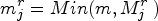
The estimation ${\hat{Y}}^{r}$ of $Y^{r}$ is computed incrementally as follows:

\begin{aligned} {\hat{Y}}^{r} = {\hat{Y}}^{r - 1} + {\hat{Y}}^{r +}, \end{aligned}

(3.1)

where

{\hat{Y}}^{0} = Y^{0}

and

{\hat{Y}}^{r +}

is computed using the Generalized Weight Share Method Estimator,⁷ where

\begin{aligned} {\hat{Y}}^{r +} = \sum_{k \in S^{r}} w_{k}^{r} y_{k}, \end{aligned}

(3.2)

and where the sampling weight

w_{k}^{r}

is given by

\begin{aligned} w_{k}^{r} = \sum_{j \in S^{r - 1}} \frac{λ_{j, k}}{L_{k}^{r - 1}} \frac{M_{k}^{r}}{m_{k}^{r}} . \end{aligned}

(3.3)

We note that inserting Expression (3.3) in (3.2), we have

\begin{aligned} {\hat{Y}}^{r +} & = \sum_{k \in S^{r}} \sum_{j \in S^{r - 1}} \frac{λ_{j, k}}{L_{k}^{r - 1}} \frac{M_{k}^{r}}{m_{k}^{r}} y_{k} = \sum_{j \in S^{r - 1}} {\hat{\bar{y}}}_{j}^{(r - 1, r) +}, where \\ {\hat{\bar{y}}}_{j}^{(r - 1, r) +} & = \sum_{k \in S^{r}} \frac{λ_{j, k}}{L_{k}^{r - 1}} \frac{M_{k}^{r}}{m_{k}^{r}} y_{k} \end{aligned}

is the unbiased sample estimate of

{\bar{y}}_{j}^{(r - 1, r) +} .

3.3 Example

To help clarify the methodological developments and the notation used, we will discuss the population depicted in Figure 2, where units B and C are selected in sample $S^{0}$ .

3.3.1 Step 1

Let us consider the case illustrated in Figure 7, where $m = 2$ .

Figure 6.

Relationship of the true total in the population and that defined at the end of the RDS process.

Let's first consider unit B of $S^{0}$ . The units that can be selected from B are A, E, and G, where, according to Table 2, we have $L_{A}^{0} = 1, L_{E}^{0} = 2, and L_{G}^{0} = 2.$ Moreover, it is $M_{B}^{1} = 3$ , and $m_{B}^{1} = M i n (3, 2) = 2.$ Moving on to the sample selection, the units that are chosen with a SRSWOR design are A and G.

Let us now consider Unit C of $S^{0}$ . The units that can be selected from C are D, E, F, and G, with $L_{D}^{0} = 1, L_{E}^{0} = 2, L_{F}^{0} = 1 and L_{G}^{0} = 2$ (see Table 2). Moreover, we have $M_{C}^{1} = 4$ , and $m_{C}^{1} = M i n (4, 2) = 2.$ The units that are chosen are G and F.

Please note that Unit G has been selected twice in the sample, highlighting the issue of multiplicity that can occur with this type of sampling.

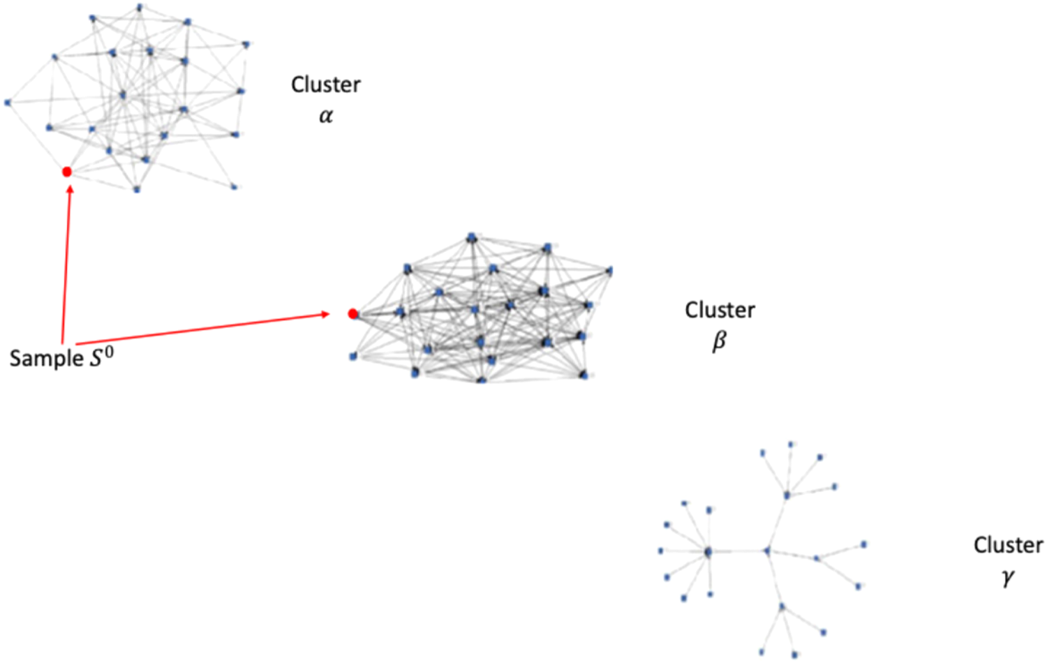
At the end of the process, sample $S^{1}$ includes units A, F, and G. Additionally, at the conclusion of this step, Units D and E, which were included in the selection lists for Units B and C, will be registered and subsequently removed from any selection lists created in the following RDS steps.

The calculus of the estimate ${\hat{Y}}^{1},$ is

\begin{aligned} {\hat{Y}}^{1} = Y^{0} + {\hat{Y}}^{1 +} = 2 + 5 = 7, \end{aligned}

Table 5 illustrates the elements for the calculus of the estimate ${\hat{Y}}^{1 +}$ .

Table 5.

Example of the calculus of ${\hat{Y}}^{1 +}$ via the indirect approach.

3.3.2 Step 2

We randomly select a sample of additional units from $S^{1}$ ( $A, F, \; and\; G$ ).

All links of units G and F are already included in sample $S^{1}$ ; therefore, no additional units are selected from these units. Unit A is the unique unit (among those new in $S^{1}$ ) from which we can proceed to a further selection step. We have $L_{I}^{1} = 1, and\; L_{H}^{1} = 1.$ Moreover, it is $M_{A}^{2} = 2$ , and $m_{A}^{2} = M i n (2, 2) = 2.$ Figure 8 and Table 6 illustrate this case.

Figure 7.

Step 1 of the sample in the RDS process.

The calculus of the estimate ${\hat{Y}}^{2},$ is

\begin{aligned} {\hat{Y}}^{2} = {\hat{Y}}^{1} + {\hat{Y}}^{2 +} = 7 + 2 = 9. \end{aligned}

3.3.3 Step 3

Both Unit I and Unit H have a single unexplored link pointing to Unit P. As a result, both Unit I and Unit H select Unit P with certainty. Figure 9 and Table 7 illustrate this case.

Figure 8.

Step 2 of the sample in the RDS process.

The calculus of the estimate ${\hat{Y}}^{3},$ is

\begin{aligned} {\hat{Y}}^{3} = {\hat{Y}}^{2} + {\hat{Y}}^{3 +} = 9 + 1 = 10. \end{aligned}

3.3.4 Closing

When restarting the RDS process, one notices that all the links of Unit P have already been explored. Hence, the RDS process ends, and we set $\hat{Y} = {\hat{Y}}^{3}$ .

4 Feasibility and outlook

This section addresses various issues that could threaten the proposed strategy. We will briefly suggest approaches to mitigate some of the problems arising from these issues. However, each topic discussed here deserves its own paper, complete with empirical and theoretical research.

Table 6.
Example of the calculus of ${\hat{Y}}^{2 +}$ via the indirect approach.

4.1 Approximation of

L_{k}^{r}

values

Estimators 3.2 (with weights given by Expression 3.3) may face computability issues because some values $L_{k}^{r}$ are unknown. This situation arises when $r \geq 1$ . However, when $r = 0$ , the quantity $L_{k}^{0}$ can be determined by collecting unique, albeit non-identifiable, information on all contacts of the units in $S^{0}$ , as well as on the contacts of the selected units in sample $S^{1}$ . Consequently, $L_{k}^{0}$ can be accurately reconstructed by performing record linkage operations on this information.

In contrast, $L_{k}^{r}$ is not known for r ≥ 0, since we observe the links only for a sample of units in $U^{r}$ . Therefore, to ensure that Estimator 3.2 is computable, we must establish a reasonable value for $L_{k}^{r}$ . We can achieve this by recognizing that $L_{k}^{r}$ is constrained by a lower and an upper bound. The lower bound, $L_{k, l o w}^{r}$ , is determined by the number of links of Unit k observed in the sample $S^{r}$ . In contrast, $L_{k} - 1$ represents the upper bound, which implies $L_{k, l o w}^{r} \leq L_{k}^{r} \leq L_{k} - 1$ .

A reasonable approximation of $L_{k}^{r}$ can be obtained using the following convex combination:

\begin{aligned} L_{k, α}^{r} = α L_{k, l o w}^{r} + (1 - α) (L_{k} - 1) \end{aligned}

(4.1)

where

0 \leq α \leq 1

is a predefined constant. By specifying the value of α, we can derive an approximate estimator, denoted as

{\hat{Y}}_{α}^{r +}

, from the correct estimator in Expression 3.2 by substituting the

L_{k}^{r}

value in Expression 3.3 with

L_{k, α}^{r}

We can determine the maximum and minimum values that the estimate ${\hat{Y}}_{α}^{r +}$ can take by setting $α$ to either 0 or 1. Specifically, ${\hat{Y}}^{r +}$ lies within the following interval: ${\hat{Y}}_{α = 0}^{r +} < {\hat{Y}}^{r +} < {\hat{Y}}_{α = 1}^{r +}$ . By knowing ${\hat{Y}}_{α = 0}^{r +}$ and ${\hat{Y}}_{α = 1}^{r +}$ , we can assess the maximum potential bias we might encounter. This is defined as the maximum absolute difference between ${\hat{Y}}_{α}^{r +}$ and both ${\hat{Y}}_{α = 0}^{r +}$ and ${\hat{Y}}_{α = 1}^{r +}$ :

\begin{aligned} B i a s_{M a x} ({\hat{Y}}_{α}^{r +}) = max (| {\hat{Y}}_{α = 0}^{r +} - {\hat{Y}}_{α}^{r +} |, | {\hat{Y}}_{α = 1}^{r +} - {\hat{Y}}_{α}^{r +} |) . \end{aligned}

(4.2)

Setting $α = 0.5$ minimizes this maximum potential bias.

4.2 Stop rule

The sampling strategy we proposed is valid only when the RDS search is exhausted. This means it is applicable only when the stopping rule is that no new units are found to include in the sample. This characteristic may make the strategy less appealing to those managing the survey, as it poses a risk of an uncontrolled increase in sampling costs.

There are some alternatives to overcome this issue. The first is to model the trend of the ${\hat{Y}}^{r}$ estimates. From a certain point onwards, these estimates should grow less and less. The researcher can model the behavior of the ${\hat{Y}}^{r}$ value curve by using a decreasing exponential function, which can help predict the curve's asymptote. This approach would allow us to conclude the RDS search earlier.

Another possible approach is to restrict the geographic size of the graph. The search for new units would stop if they fall outside the predefined geographical boundary of the network. In other words, a network spanning two distinct geographic locations can be analyzed as two separate networks. To implement this approach, the sampling design can be structured as a two-stage (or two-phase) process. In the first stage, a sample of geographic locations is selected. In the second stage, the RDS search is conducted within these selected locations, ensuring that contacts living outside the geographical boundaries are not explored. However, this method necessitates identifying seeds for each first-stage sample unit. To reduce economic and operational costs, first-stage units can be selected with a probability proportional to the concentration of the target population in each area, provided this quantity is known. Alternatively, if these concentrations are unknown or only approximately known, they can be classified using an ordinal scale, assigning higher selection probabilities to PSUs associated with higher values on the scale.

Table 7.
Example of the calculus of ${\hat{Y}}^{3 +}$ via the indirect approach.

4.3 Data needed for carrying out the survey operations

One of the main challenges is obtaining the data necessary for both sample selection and estimate construction. In the described procedure, the surveyor must identify selectable units from the list of units associated with a given sample unit. This step can be performed in real time during the interaction with the respondent, but only if the interview is conducted using computer-assisted methods. Furthermore, the interview application must store historical data to differentiate between individuals listed by the current sample unit and those recorded in previous RDS steps.

Alternatively, after collecting the respondents’ contact information, the researcher can forward this data to the survey's central processing unit. The central unit would then carry out linkage operations to identify units previously mentioned by other respondents and generate a random list of new units for the researcher to contact.

A key challenge related to the previously mentioned topic is the need to divide the survey into distinct steps. This subdivision can be particularly difficult if enumerators in the field are expected to carry it out independently. From an operational perspective, these steps can be organized in a chronological sequence—for instance, initiating a new step every two days. After completing each step, enumerators must download the data on the contacts and respondents collected during the interviews. This information must then be properly processed, including performing record linkage operations, to ensure that enumerators can clearly define the list of selectable units for the next step.

5 Empirical analysis

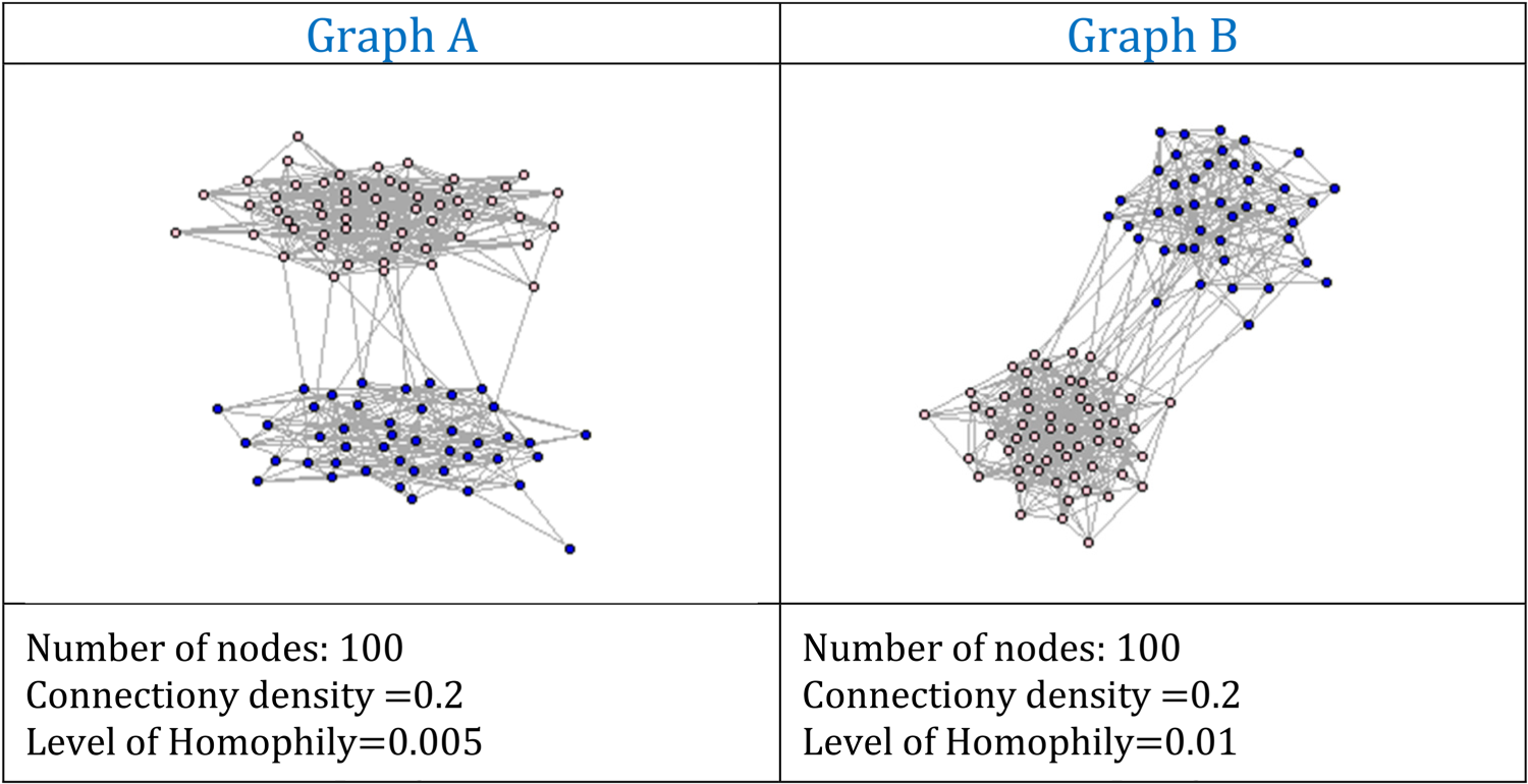
A simulation study was conducted using the R statistical software to evaluate the properties of the sampling method presented in the paper. The simulation aims to validate the proposed estimation strategy by examining two types of graphs, referred to as Graph A and Graph B, each featuring varying degrees of homophily and a moderate level of complexity. The number of units in each graph was set to 100.

Each graph is divided into two distinct groups, each with a connection density—defined as the probability of connection between two units within the same group—of 0.2. Graph A has a level of homophily, or the probability of connection between the two groups, set at 0.005. In contrast, Graph B has a level of homophily of 0.01.

Figure 10 below represents the two graphs, summarizing their characteristics.

Figure 9.

Step 3 of the sample in the RDS process.

On each of these two graphs, we applied two RDS processes. In the first process, we selected a single initial seed, while in the second process, we selected two initial seeds. For each subsequent RDS steps, the number of units selected ( $m$ ) was consistently set to 2.

By analyzing the characteristics of the graphs and the RDS process, we have considered four distinct scenarios in total, as shown in Table 8 below.

Table 8.

Characteristics of scenarios.

Scenarios	Graph	Initial seeds
1	A, Homophily 0.005	1
2	A, Homophily 0.005	2
3	B, Homophily 0.01	1
4	B, Homophily 0.01	2

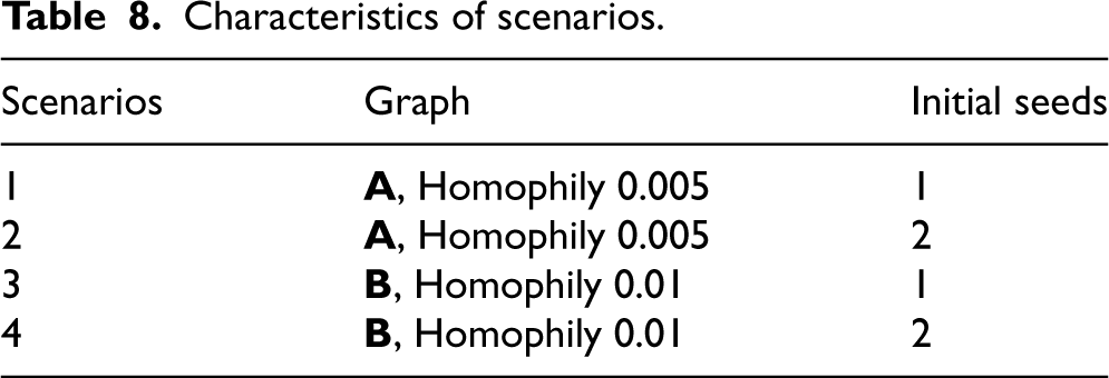
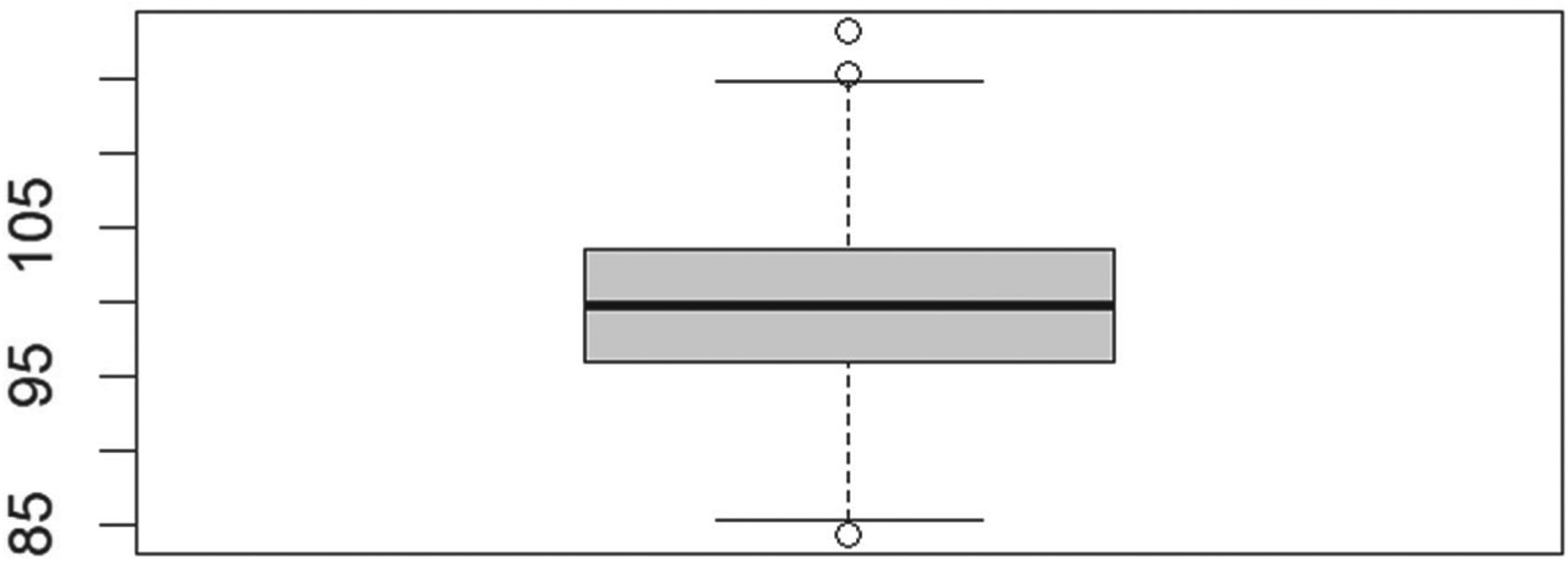
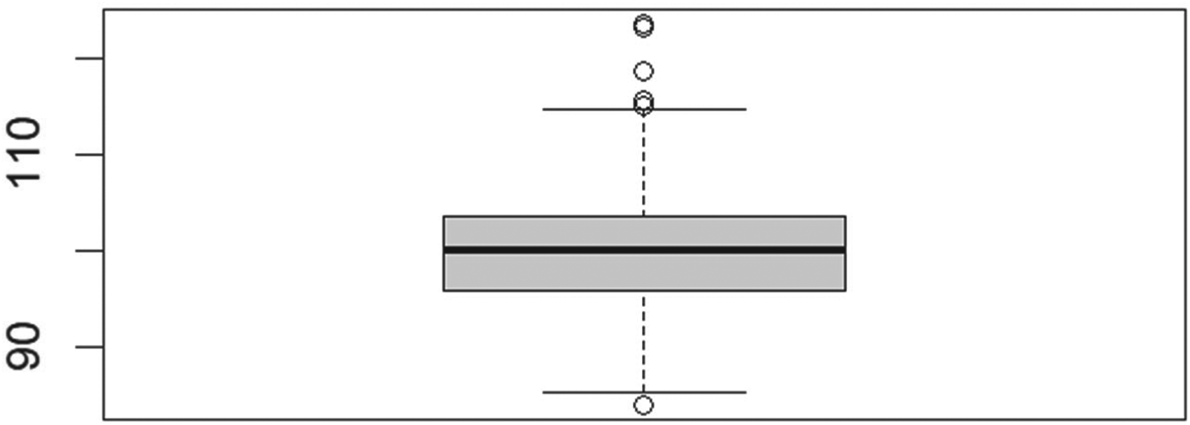
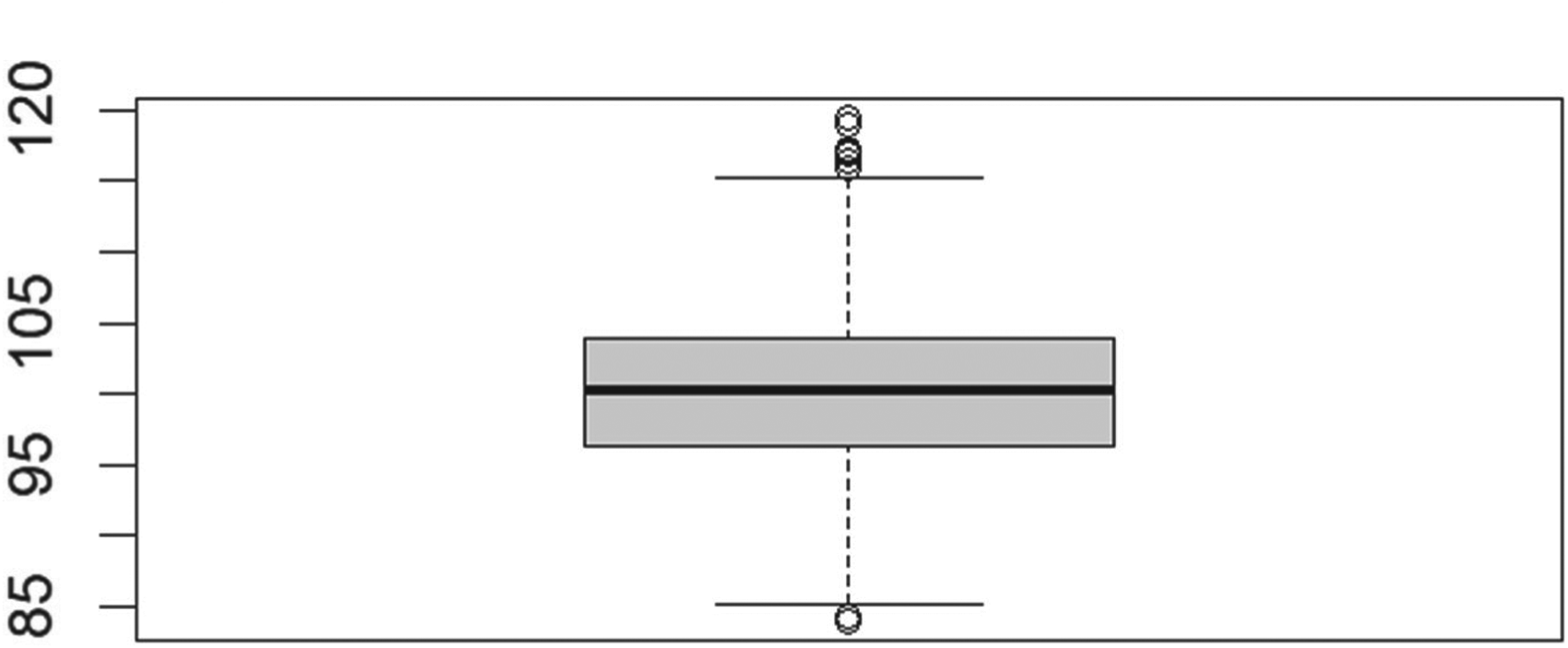
We simulated four scenarios, conducting 1000 RDS (Respondent-Driven Sampling) search processes (iterations) as detailed in Section 3. The initial number of seeds was consistent for scenarios 1 and 3, as well as for scenarios 2 and 4. At the end of each iteration, we calculated the GWSE (Generalized Weighted Sampling Estimates) for the total population, which is set at 100. A summary of the results can be found in Table 9, while Figures 11 to 14 illustrate the box plots of the sampling estimates for each scenario.

Figure 10.

Representation of the 2 population schemes considered.

Figure 11.

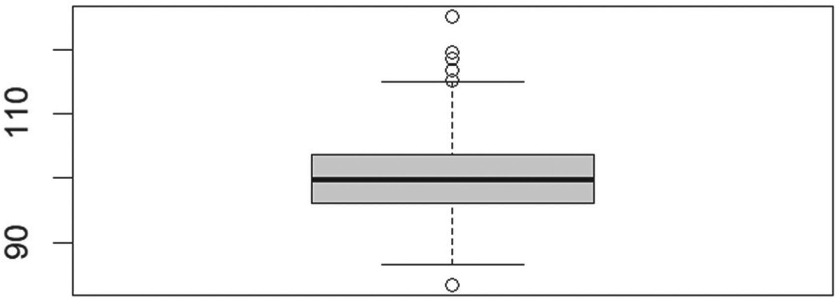
Boxplot of Scenario 1 showing the total population estimates. Homophily = 0.005, #Seeds = 1.

Figure 12.

Boxplot of Scenario 2 showing the total population estimates. Homophily = 0.005, #Seeds = 2.

Figure 13.

Boxplot of Scenario 3 showing the total population estimates. Homophily = 0.01, #Seeds = 1.

Figure 14.

Boxplot of Scenario 4 showing the total population estimates. Homophily = 0.01, #Seeds = 2.

Table 9.

Summary of results by scenario.

Scenario	Min	1° Quantile	Median	Mean	3° Quantile	Maximum	CV (%)
1 Homophily = 0005 Seeds = 1	83.35	96.09	99.75	100.10	103.73	125.19	5.56
2 Homophily = 0005 Seeds = 2	84.42	96.01	99.75	99.84	103.68	118.28	5.47
3 Homophily = 0,01 Seeds = 1	83.93	95.92	99.94	99.93	103.56	123.63	5.67
3 Homophily = 0,01 Seeds = 2	83.96	96.34	100.13	100.25	103.99	119.48	5.66

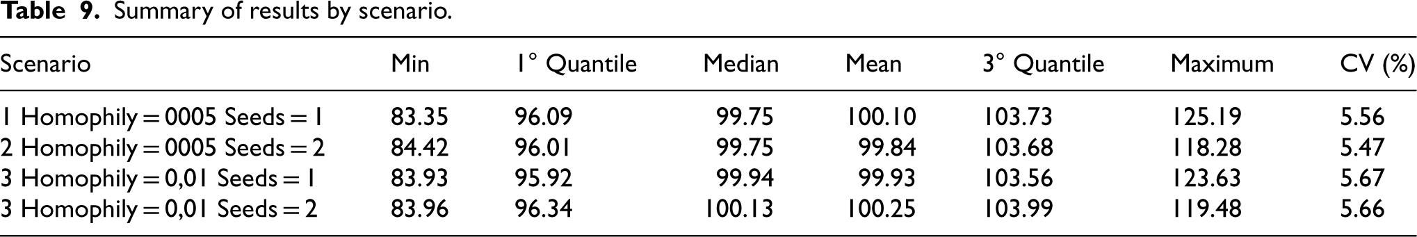
The results we obtained are very encouraging. We have successfully demonstrated the fundamental outcome we aimed to achieve: our proposed method generates unbiased estimates of the total population across each of the four scenarios.

The coefficients of variation (CVs) of the estimates remain consistent, although selecting only two initial seeds helps limit extreme outlier values. Furthermore, in all four scenarios, the variability of the estimates between the first and third quartiles is minimal.

These initial findings are indeed promising. To enhance the robustness of our methodological proposal, we will need to conduct further experiments based on the guidance provided in Section 4 of this work.

6 Conclusions

Disaggregating data for SDG indicators on hard-to-reach populations presents several critical challenges that are difficult to overcome within the current framework of official statistics in many countries. In this context, estimating the characteristics of such populations using traditional modeling approaches is not feasible.

Therefore, it is crucial to define and implement a sampling strategy that can effectively address this issue. Priority should be given to sampling designs that maximize the number of observed individuals within the target population.

Respondent-driven sampling (RDS), which leverages existing social connections within the target population, proves to be a valuable tool for surveying these groups and providing approximate estimates of their actual size.

The article discusses the challenges involved in estimating totals within RDS and proposes a new methodological framework to address these issues. After outlining the limitations of traditional techniques, the authors introduce an innovative approach that utilizes indirect sampling methods. They clarify the practical requirements for implementing this new method, which includes collecting contact information and performing linkage operations to identify previously sampled units.

The methodology was validated through simulations and empirical applications, demonstrating its effectiveness and reliability. This approach offers a robust and practical solution to overcome the shortcomings of traditional RDS estimates, ensuring greater accuracy and applicability in complex network settings.

The findings we obtained are preliminary but show significant promise. To enhance the reliability of our proposed methodology, additional experiments should be conducted following the recommendations outlined in Section 4 of this study.

The research team is currently conducting additional experiments using simulated data, and the findings will be presented in a new paper.

Footnotes

ORCID iD

Giorgio Alleva

Funding

The authors received no financial support for the research, authorship, and/or publication of this article.

Declaration of conflicting interests

The authors declared no potential conflicts of interest with respect to the research, authorship, and/or publication of this article.

References

Gile

Beaudry

Handcock

, et al. Methods for inference from respondent-driven sampling data. Annu. Rev. Stat. Appl 2018; 5: 1–429. 2018.

Heckathorn

Cameron

. Network sampling: from snowball and multiplicity to respondent-driven sampling. Annu Rev Sociol 2017; 43(1): 101–119.

Heckathorn

. Respondent driven sampling: a new approach to the study of hidden samples. Soc. Probl 1997; 44: 174–199.

White

Hakim

Salganik

, et al. Strengthening the reporting of observational studies in epidemiology for respondent-driven sampling studies: “STROBE-RDS” statement. Journal Clinical Epidemiology 2015 Dec; 68: 1463–1471. 2015.. Epub 2015 May 1. https://pubmed.ncbi.nlm.nih.gov/26112433/-full-view-affiliation-2

Shi

Cameron

Heckathorn

. Model-based and design-based inference: reducing bias due to differential recruitment in respondent-driven sampling. Sociol. Methods Res 2016; 48(1).

Falorsi

Alleva

Petrarca

. Unbiased estimation strategies for respondent driven sampling. Stat J IAOS Stat 2024; 1: 1–12.

Lavallée

. Indirect Sampling. New York: Springer, 2007.

	$U$
	A	B	C	D	E	F	G	H	I	L	R	M	N	O	P
A	1	1	0	0	0	0	0	1	1	0	1	0	0	0	0
B	1	1	0	0	1	0	1	0	0	0	0	0	0	0	0
C	0	0	1	1	1	1	1	0	0	0	0	0	0	0	0
D	0	0	1	1	0	0	0	0	0	1	0	1	0	0	0
E	0	1	1	0	1	0	0	0	0	0	0	0	0	0	0
F	0	0	1	0	0	1	0	0	0	0	1	0	0	0	0
G	0	1	1	0	0	0	1	0	0	0	0	0	0	0	0
H	1	0	0	0	0	0	0	1	0	0	0	0	0	0	1
I	1	0	0	0	0	0	0	0	1	0	0	0	0	0	1
L	0	0	0	1	0	0	0	0	0	1	0	0	1	0	0
M	0	0	0	1	0	0	0	0	0	0	0	1	0	1	0
N	0	0	0	0	0	0	0	0	0	1	0	0	1	0	0
O	0	0	0	0	0	0	0	0	0	0	0	1	0	1	0
P	0	0	0	0	0	0	0	1	1	0	0	0	0	0	1

	$U$
	A	B	C	D	E	F	G	H	I	L	R	M	N	O	P
A	1	1	0	0	0	0	0	1	1	0	1	0	0	0	0
B	1	1	0	0	1	0	1	0	0	0	0	0	0	0	0
C	0	0	1	1	1	1	1	0	0	0	0	0	0	0	0
D	0	0	1	1	0	0	0	0	0	1	0	1	0	0	0
E	0	1	1	0	1	0	0	0	0	0	0	0	0	0	0
F	0	0	1	0	0	1	0	0	0	0	1	0	0	0	0
G	0	1	1	0	0	0	1	0	0	0	0	0	0	0	0
H	1	0	0	0	0	0	0	1	0	0	0	0	0	0	1
I	1	0	0	0	0	0	0	0	1	0	0	0	0	0	1
L	0	0	0	1	0	0	0	0	0	1	0	0	1	0	0
M	0	0	0	1	0	0	0	0	0	0	0	1	0	1	0
N	0	0	0	0	0	0	0	0	0	1	0	0	1	0	0
O	0	0	0	0	0	0	0	0	0	0	0	1	0	1	0
P	0	0	0	0	0	0	0	1	1	0	0	0	0	0	1

Building estimates for totals in respondent driven sampling

Abstract

Keywords

1 Introduction

2 The RDS research path

Proof of Formulae 2.4, 2.5 and 2.6. Proof of Formulae 2.4, 2.5 and 2.6.

2.3 Step 2

Table 3. Example of the calculus of Y 2 via the indirect approach.

2.6 Caveat

3.1 Sampling process

3.3.1 Step 1

4 Feasibility and outlook

Table 6. Example of the calculus of Y ^ 2 + via the indirect approach.

Table 7. Example of the calculus of Y ^ 3 + via the indirect approach.

5 Empirical analysis

Footnotes

ORCID iD

Funding

Declaration of conflicting interests

References

Table 3.
Example of the calculus of $Y^{2}$ via the indirect approach.

Table 6.
Example of the calculus of ${\hat{Y}}^{2 +}$ via the indirect approach.

Table 7.
Example of the calculus of ${\hat{Y}}^{3 +}$ via the indirect approach.

	$U$
	A	B	C	D	E	F	G	H	I	L	R	M	N	O	P
A	1	1	0	0	0	0	0	1	1	0	1	0	0	0	0
B	1	1	0	0	1	0	1	0	0	0	0	0	0	0	0
C	0	0	1	1	1	1	1	0	0	0	0	0	0	0	0
D	0	0	1	1	0	0	0	0	0	1	0	1	0	0	0
E	0	1	1	0	1	0	0	0	0	0	0	0	0	0	0
F	0	0	1	0	0	1	0	0	0	0	1	0	0	0	0
G	0	1	1	0	0	0	1	0	0	0	0	0	0	0	0
H	1	0	0	0	0	0	0	1	0	0	0	0	0	0	1
I	1	0	0	0	0	0	0	0	1	0	0	0	0	0	1
L	0	0	0	1	0	0	0	0	0	1	0	0	1	0	0
M	0	0	0	1	0	0	0	0	0	0	0	1	0	1	0
N	0	0	0	0	0	0	0	0	0	1	0	0	1	0	0
O	0	0	0	0	0	0	0	0	0	0	0	1	0	1	0
P	0	0	0	0	0	0	0	1	1	0	0	0	0	0	1