Conceptualizing economic leading indicators for early warning of Thailand's business cycle turning points

Abstract

The research utilized official statistical data for economic early warning. Several data were narrowed down to eight potential leading indicators regarding their cycle relationship to Thailand's business cycle from 1993Q1 to 2022Q4. Instead of using Principal Component Analysis (PCA) for indicator selection, this study derived underlying dimensions of selected leading indicators in broader concepts than monitoring individuals, enhancing the understanding and interpretation. Those eight indicators were classified and constructed into the three Composite Leading Indexes (CLIs); additionally, all were aggregated to be a single CLI as a benchmark. In evaluating CLIs’ real-time forecasting, the results showed that using the three component-specific CLIs complementarily provides better performance than including all of them in a single CLI or relying solely on the first component from PCA. As for the benefit of policy implementation, since peaks can probably cause more severe economic damage than troughs, policymakers should prioritize CLI representing “Economic Activity Driver” to mitigate damage from economic peaks, as it tracks production and business sentiment. The second, capturing “Economic Investment Trend,” monitors investment dynamics, while the third, providing “Economic Price Pressure,” reflects inflation and declining wealth. Monitoring these three CLI provides insights into economic growth and policy interventions.

Keywords

Business cycle double one-sided Hodrick-Prescott leading indicator multivariate analysis principal component analysis

1. Introduction

Minimizing economic fluctuations has always been a priority for policymakers. Understanding and predicting the economy through analyzing a business cycle of official statistical data is essential for this task.

The modern theory of economic cycles is often associated with the business cycle concept developed by Burns and Mitchell,¹ which used a classical approach based on trend-cyclical data, defining business cycles as sequences of expansions and contractions in key economic indicators. This empirical framework is widely adopted by several developed countries.^2,3

In the case of emerging countries with high volatility, the linear term of the classical approach may not be appropriate because it might not capture cyclical stages.⁴ The growth cycle approach of Mintz⁵ is the optional solution for emerging countries,⁶ which is similar to the classical approach; the only difference is that this approach, based on de-trended data, uses filtering techniques extracting the cyclical component out of the time series to measure deviations from long-term trends. Based on previous research on Thailand's business cycle, this study adopted the growth cycle approach, which is suitable for emerging economies like Thailand.^7,8

Policymakers have long paid attention to developing an Early Warning System (EWS) to signal business cycle turning points since it aids them in implementing timely economic policy. Considerable literature has been studied to determine reliable economic predictions since the pioneering research of Mitchell and Burns,⁹ who proposed identifying leading indicators. However, only one leading indicator may not completely signal the economic cycle over a given period; monitoring several indicators without having synthetic information analysis might not be the best solution as well.¹⁰ Therefore, much research followed the remarkable work of Stock and Watson,¹¹ who proposed constructing a Composite Leading Index (CLI) by aggregating some leading indicators to improve a more comprehensive measure of economic activity and facilitate the policymaker. Nevertheless, there can be various prospective leading indicators; combining all of them as one CLI may not be the optimal solution since each might have unique characteristics, and some might have similar features.

Many studies applied Principal Components Analysis (PCA), a dimensionality reduction technique following Stock and Watson,¹² to select some leading indicators that should be aggregated as a CLI by using only the first principal component.^13,14 However, this study did not focus solely on leading indicator selection; the interest was also in deriving underlying dimensions of those potentially selected leading indicators, which would aid the analysis for understanding and interpreting them in broader concepts than monitoring individual leading indicators. Afterward, the research extended the data summarization process by deriving an empirical value for each dimension as a CLI to substitute the individual leading indicators with these more concise dimensions.

As for Thai literature, the business cycle concept was considerably applied related to the monetary and financial sectors.^15,16 However, there has been less focus on early warning in the real business cycle, although some work has been done in this area. One example is the monthly frequency data named the leading economic index (LEI) developed by the Bank of Thailand. It includes seven indicators: Authorized capital of newly registered companies, Permitted new construction area, Export volume index (exclude gold), Business sentiment index (BSI) (expectation next 3 months), SET index, Real broad money, and Oil price inverse index (Dubai). Its methodology uses the Coincident economic index as the referent series of the economy, which aims to forecast Thailand's economy in the short term (3 to 4 months).¹⁷

Even monthly data might provide more timely signals compared to quarterly data. However, the Gross Domestic Product (GDP), available on a quarterly basis, is the most common proxy for economic activities to monitor the economic cycle since it is usually considered the broadest indicator of economic activity.^18–20 As a result, much of the literature on monthly data tries to identify or construct indicators that strongly correlate with GDP to represent economic activity.^18,19

Therefore, this research aimed to construct quarterly CLIs that applied GDP as a reference for Thailand's economic activities and provide early signals of turning points in the medium term, which could forecast the Thai economy 3 to 4 quarters ahead. Rather than incorporating all potential leading indicators into a single CLI, this study applied PCA to identify underlying dimensions, thereby simplifying the data into fewer concepts for easier interpretation and facilitating policymakers’ decision-making.

2. Background

2.1 Reference series

The key purpose of economic leading indicators is to signal or predict economic activity. From this perspective, selecting a proxy for economic activity is a crucial first step, referred to as the reference series. The use of the referent index is to monitor fluctuations in economic activity and determine turning points in the business cycle, which assesses the current position of the economy and its future direction, making it useful for forecasting purposes.

The GDP and Industrial Production Index (IPI) are typically used as a reference series to measure economic activity.¹⁰ However, GDP is officially available quarterly; many who aim for monthly frequency basis analysis prefer IPI.^14,19 Some might apply a latent variable obtained by many relevant economic indicators called the Coincident economic index since they reasoned that it covers the multidimensional aspect of economic activity more than IPI.^13,17

However, this research restricted the attention to GDP, which is usually considered the broadest indicator capturing economic activity and the most common use as a proxy of the economy.^18–20 Moreover, compared to IPI, GDP has the advantage of more comprehensive economic coverage; for some countries, IPI does not provide information as a proxy but as the economic leading indicator.¹⁸ In addition, much previous literature related to Thailand's economy has also used GDP as the reference series.^8,20

2.2 Potential leading indicators

One of the most widely used EWS tools is the leading indicators, pioneered by Mitchell and Burns,⁹ aiming to predict future recessions and recoveries of the economy. As for leading indicators, some might use all variables in a selected database and add transformations. Many began with a systematic literature review^21,22 and a theory-based study,^23,24 then narrowed down a set of useful indicators. However, the limitations of these studies were based on their search, risking overlooking critical leading indicators; many researchers included additional leading indicators based on their judgment to mitigate this risk.²⁵ In other words, some selected indicators mainly rely on empirical properties and might be less on theoretical bases. These chosen leading indicators should be accompanied by an explanation of the economic basis for their potential correlation with economic activity. Besides being economically significant, practical considerations should also be taken into account — not subject to major revisions (i.e., stability), timely, long-time series with no breaks, and, more importantly, having the cyclical movements preceding the reference series.^14,19

Nevertheless, there are a large number of variables that could be leading indicators. Hence, most researchers usually start with the literature review to identify useful leading indicators and then use econometric or statistical techniques to narrow them down,¹³ such as Cross-correlation analysis, Turning point analysis, Probit model, and Granger causality tests.

2.3 Composite leading index

Because of the unique characteristics of each indicator, solely one indicator cannot explain the fluctuation of the reference cyclical over a particular period since each has its own potential depending on the cycle. As proposed by Stock and Watson,¹¹ aggregating indicators into a Composite index can better explain economic fluctuations than a single indicator. Instead of using individual leading indicators separately, analysts typically combine them into CLIs based on their leading ability horizon to capture a broader range of factors that influence the cyclical changes of the economy.

2.4 Principal component analysis

In most cases, there will be many useful leading indicators; aggregating all of them into one CLI might not be an optimal solution. The challenge is to select the most appropriate leading indicators for constructing CLIs. Much literature has addressed this challenge by applying Multivariate analysis to identify the underlying data structure and reduce its dimensionality, making the indicator selection more efficient.

Regarding data reduction techniques, Common Factor Analysis focuses only on common (shared) variance, assuming that unique and error variances do not contribute to determining the structure of variables in the analysis. On the other hand, PCA is a method that considers total variance, including both common and unique, to derive components.²⁶ As for the application, some research has applied Common Factor Analysis to identify indicator components of the Coincident index,²⁷ and much of the literature on the CLI has used PCA to select leading indicators.^12–14,28

As for the PCA technique, it estimated linear combinations of the original indicators $(X_{i}, i = 1, 2, \dots, r)$ as the new variables–Principal Component (PC) $(P C_{j}, j = 1, 2, \dots, q : q \leq r)$ .

\begin{aligned} P C_{j} = l_{j 1} X_{1} + l_{j 2} X_{2} + \dots + l_{j r} X_{r}; j = 1, 2, \dots, q : q \leq r \end{aligned}

(1)

l_{j i}

is the loadings or weight of each original variable to construct

P C_{j}

. Whereas PC₁ extracted the largest possible variance, PC₂ absorbed the greatest possible variance of the leftover from PC₁, and this process continues sequentially until the last PC extracts the remaining variance.

3. Empirical analysis

3.1 Data preparation

The research aimed to identify leading indicators to predict turning points in Thailand's business cycle, using GDP as the reference series. Hence, possible leading indicators were collected from a broad range of monetary, financial, real economic, and related variables, totaling 100 indicators (excluding the reference variable). This selection was based on previous literature and further adjusted by the researcher. The data range covered 1993Q1 to 2022Q4, as the first GDP data was available from 1993Q1. However, due to variations in data availability, some datasets were published after 1993Q1, resulting in a differing time span for certain data. Since this study focused on quarterly frequency, if the collected data were available monthly, it would be transformed by basic approaches, including average, summation, or end-of-period. The average method was most frequently applied since it is suitable for many economic series related to rates, prices, and indices. Whereas summation is aligned with the flow data (e.g., production, trade), the end-of-period commonly uses the last month of the quarter to represent the entire quarter (e.g., stock levels).

As this study adopted the growth cycle concept, the deviation-from-trend, the filtering techniques were applied to remove other time series factors that could vague the cyclical patterns. For series displaying an explicit seasonal pattern, X-13 adjustment would be performed prior to the de-trending process. Cycle extraction plays a crucial role in business cycle analysis, and many statistical techniques have been proposed for de-trending to extract the cyclical component.

Hodrick-Prescott (HP)^29,30 has been popular for the task, especially for studying business cycles in an emerging economy,⁶ because it is considered a simple and effective filtering technique.³¹ The HP decomposes the series into a trend and a cyclical component, which aims to minimize the distance between the trend and the initial series while minimizing the curvature of the trend. The method requires only the smoothing parameter to optimize the trade-off between these two aims. This smoothing parameter is related to the smoothness degree of the estimated trend, in which the larger value will produce more smoothness. The empirical guidelines suggest setting the smoothing parameter as 14,400, 1,600, and 100 for monthly, quarterly, and annual data, respectively.³² Many works increase the stability of the cyclical estimation by applying HP twice, called Double Hodrick-Prescott (DHP).^19,33 However, the HP result has been criticized. Some critics indicate that HP's dependency on using the full sample (past and future observations) results in spurious dynamic relations (spurious predictability), including an end-point problem (significant reversion), in that the filtered values have high differences between the sample's middle and end; the revision estimated trend and cyclical components happened when new data is available.^7,34

Due to the criticism of the HP method, which happened from using the full sample in analysis, this study considered applying the One-sided Hodrick-Prescott (OneHP)³⁰ that uses only a partial sample (past to present observations) for estimating trend and cyclical components, which may suffer less from spurious predictability or end-point biases as HP. Furthermore, to enhance the stability of the cyclical component, the research applied it twice–Double One-sided Hodrick-Prescott (DoneHP). Moreover, the previous research on the economic cycles of Thailand indicated that this method produces fewer revisions in the estimated cycles, particularly at the end-points, compared to the filter method of HP, DHP, and OneHP.⁷ Additionally, since some indicators originated from different units or scales, standardization was applied to ensure consistency, with each indicator having a mean of 0 and a standard deviation of 1, for further conducting PCA and aggregating CLI. Without standardization, the indicators with smaller amplitudes in the CLI could be overshadowed by those with larger amplitudes. The example of filtering results, the cyclical component with strandardization, compared to the initial data, were presented in Appendix A (Figure A1).

3.2 Identification of potential leading indicators

The Cross-correlation analysis can help test the leading property and narrow down the useful leading indicators.^19,35 This study applied the method to evaluate the conformity of the cyclical movement between a pair of GDP and selected indicators, which considered the correlation between them over the entire series. If their cyclical movement is highly correlated, it would imply that selected indicators provide a signal to the entire cycle and approaching turning points.¹⁹ Moreover, the position of the highest correlation can be used to identify the lead, lag, or coincident time on average.¹⁹ It is noteworthy that cross-correlation traditionally assumes data to be well-behaved, such as stationary and normality; however, economic time series often deviate from these ideal conditions. Despite this, cross-correlation remains a widely accepted method for identifying leading indicators in economic research, as supported by studies like.^19,35 However, to ensure reliable results, the study conducted Augmented Dickey-Fuller (ADF) for a preliminary check of stationarity to validate the data's behavior.

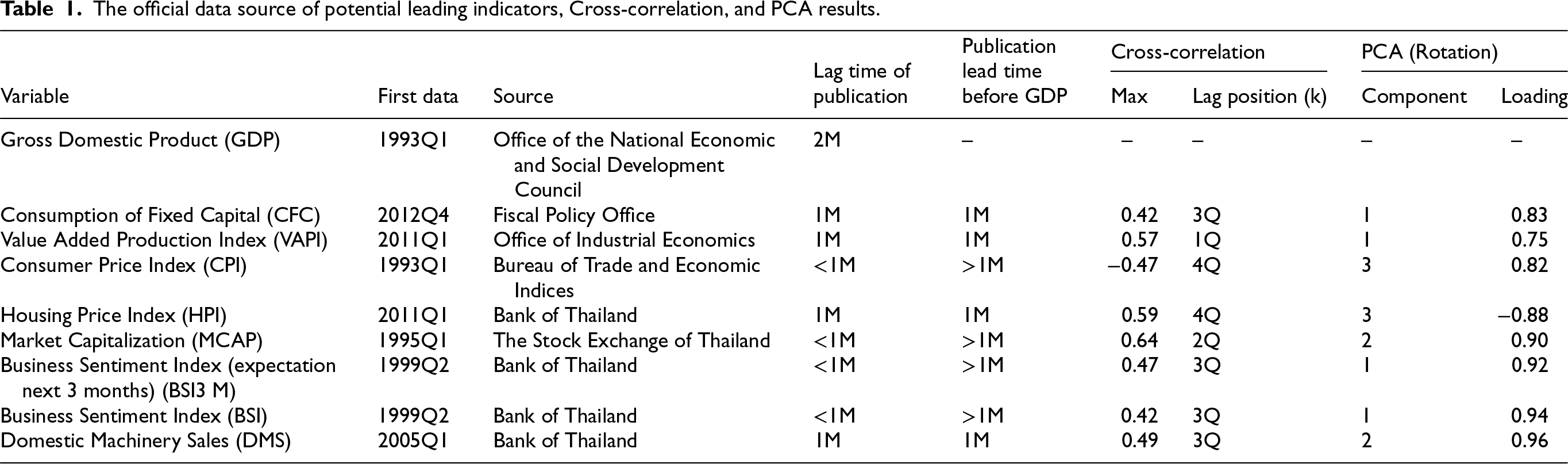
The cross-correlation was estimated between GDP and those useful leading indicators for i = 1,…,100. The position of the highest cross-correlation (k) helps identify the indicator behavior approaching GDP. If k is positive, negative, or zero, indicating that the indicator behaves as a leading, lagging, or coincident. Meanwhile, the size of the highest cross-correlation could infer how much the indicators’ cyclical profiles match. As for potential leading indicators, the highest cross-correlation with GDP should be higher than a threshold of 0.40, following the guidelines of Fiorentini and Planas.³⁶ This benchmark is based on empirical evidence rather than a strict statistical criterion, which does not account for differences in sample sizes across series or incorporate adjustments for multiple testing corrections. In addition, the position of the highest value should be over 0 (k > 0).^35–37 These selected leading indicators were also summarized as pro-cyclical (positive correlation) or counter-cyclical (negative correlation) regarding their cyclical fluctuation with GDP by their highest cross-correlation.

\begin{aligned} ρ_{(G D P, X i)} (k) = \frac{C o v (G D P_{t}, X i_{t - k})}{\sqrt{V a r (G D P_{t}) V a r (X i_{t})}} \end{aligned}

(2)

When considering the location of the highest cross-correlation within 4 periods (maximum of k is 4–four-period forward and backward), there were 44 indicators for negative k (lagging) and 23 indicators for k at zero (coincident). The rest of them, for 33 indicators, showed the highest correlation at the k-positive location, of which 13 had the highest correlation over the guideline threshold of 0.40.

Nevertheless, five of those 13 indicators were highly correlated or would be compensated by the other, nearly capturing the same economic aspect, resulting in redundancy. Based on the researcher's judgment, eight variables were selected as potential leading indicators. The five redundancy variables could be explained as follows: The Value Added Production Index (VAPI) was chosen instead of the VAPI with seasonal adjustment and the Production Value Index. The reason for selecting VAPI over its seasonal adjustment version was the preference for the consistent seasonal adjustment method across all variables if needed. 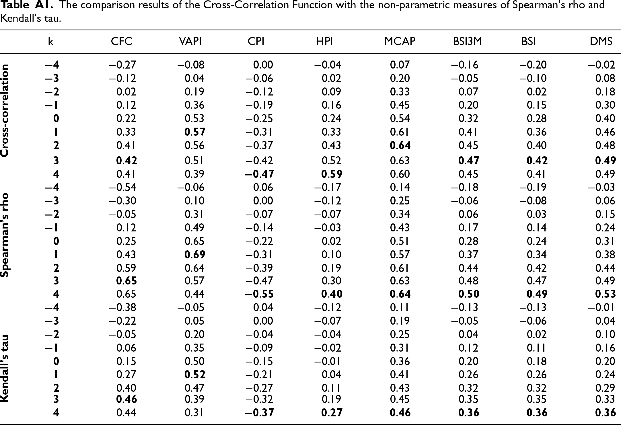As for the Production Value Index, VAPI can provide insights into production efficiency rather than just output. Additionally, their cyclical series were highly correlated at over 0.9. Meanwhile, the BSI was selected instead of the Sentiment for Total Order Book and Investment, as it offers a broader measure of business confidence, and they had strong correlations between 0.84–0.91. Lastly, the reason for selecting Market Capitalization (MCAP) over the Equity Market Index was because it could reflect a wider view of the market value, and they were correlated at 0.76. Besides, most selected indicators have greater the highest cross-correlation with GDP than their candidate.

As for clarifying the robustness of the selected eight indicators in Table 1 and enhancing the transparency of the signal strength compared to other lags, the results of a Cross-Correlation Function (CCF) were compared to the non-parametric measures of Spearman's rho and Kendall's tau as shown in Appendix A (Table A1). The results indicated that they were robust as leading indicators preceding GDP. However, the lag times exhibited vary, which might be due to the different sensitivities of the methods. Nevertheless, the research used the leading period based on the Cross-correlation analysis since the primary check indicated that all eight indicators were stationary, and seven of them explicated normality and no outlier, except Consumption of Fixed Capital (CFC) (more detail in section 3.3.2); however, the three methods agreed at the same leading periods for CEC, inferring the robust results.

Table 1.

The official data source of potential leading indicators, Cross-correlation, and PCA results.

					Cross-correlation		PCA (Rotation)
Variable	First data	Source	Lag time of publication	Publication lead time before GDP	Max	Lag position (k)	Component	Loading
Gross Domestic Product (GDP)	1993Q1	Office of the National Economic and Social Development Council	2M	–	–	–	–	–
Consumption of Fixed Capital (CFC)	2012Q4	Fiscal Policy Office	1M	1M	0.42	3Q	1	0.83
Value Added Production Index (VAPI)	2011Q1	Office of Industrial Economics	1M	1M	0.57	1Q	1	0.75
Consumer Price Index (CPI)	1993Q1	Bureau of Trade and Economic Indices	<1M	>1M	−0.47	4Q	3	0.82
Housing Price Index (HPI)	2011Q1	Bank of Thailand	1M	1M	0.59	4Q	3	−0.88
Market Capitalization (MCAP)	1995Q1	The Stock Exchange of Thailand	<1M	>1M	0.64	2Q	2	0.90
Business Sentiment Index (expectation next 3 months) (BSI3 M)	1999Q2	Bank of Thailand	<1M	>1M	0.47	3Q	1	0.92
Business Sentiment Index (BSI)	1999Q2	Bank of Thailand	<1M	>1M	0.42	3Q	1	0.94
Domestic Machinery Sales (DMS)	2005Q1	Bank of Thailand	1M	1M	0.49	3Q	2	0.96

In addition to their leading capacity, the timeliness of publication is the key concern when using these indicators for economic early warning. Approximately, GDP is typically released with a lag of about 50 days (roughly 2 months). In contrast, the eight leading indicators are published around the 1-month delay, providing information 1 month ahead of the GDP release (Table 1).

3.3 Dimensional reduction of potential leading indicators

Because of the distinct characteristics of each potential leading indicator, a single indicator cannot capture the economic cyclical fluctuation over time. Combining multiple leading indicators might help enhance the predictive performance; however, aggregating all eight indicators into one CLI might not yield the optimal result. Therefore, this research employed PCA to reduce dimensionality and classify indicators into smaller subsets based on their business cycle characteristics, representing various economic aspects.

3.3.1 PCA objectives

Instead of using PCA for selecting indicators by taking only the first component as much previous literature,^13,14 this research applied this Multivariate method summarizing potential leading indicators into fewer dimensions to understand whether these indicators can be aggregated for prediction purposes.

3.3.2 Statistical assumptions in PCA

To ensure reliable results, the statistical issues should be verified before conducting PCA.

One is multivariate normality, as tail dependence could be a factor causing non-normality, which may impact the results of PCA and other hypothesis tests. Even normality is not a strict concern for PCA.²⁶ This study diagnosed individual leading indicators’ distribution by the Jarque-Bera Test due to its simplicity instead of multivariate normality tests. The results indicated no evidence to reject the null hypothesis of normality for most series at a significance level of 0.01, with p-values ranging from 0.0381 to 0.633, except for CFC. Since outliers can also distort the PCA's results, the study addressed this issue with standardized scores. As for identifying extreme values that deviate significantly from the mean, a common threshold for detecting outliers is a standardized score beyond −3 or +3. The results indicated that most indicators fell within this range, which showed no significant outliers, except for the CFC. Its outlier exhibited in 2017Q3 likely contributed to non-normal distribution; removing this outlier resulted in returning to the normal distribution, thereby supporting the validity of the results.

Despite the non-normality and presence of outliers in the CFC, the research decided to include it in the analysis without applying any transformation. The rationale was to preserve the original character of its business cycle pattern, and the primary purpose of studying PCA in this research was to uncover underlying dimensions in the data to gain exploratory insights into the structure of leading indicators rather than make strict statistical inferences as supported by Hair, Black.²⁶ Additionally, economic time series often deviate from these ideal assumptions, and some research applying PCA in business cycles did not exclude extreme values or outliers from the analysis^13,38 since they may provide valuable insight into significant phenomena.

The next critical aspect to consider was data independence. Since this study involved time series data, which often exhibits serial correlation, the ADF without intercept and trend was performed to assess the stationarity of the standardized cyclical patterns. The results rejected the null hypothesis at a significance level of 0.05 (with p-values ranging from 0.0001 to 0.0038), indicating that all data series were stationary.

Although the critical assumptions of PCA emphasize conceptual aspects over statistical requirements,²⁶ this research focused primarily on the degree of multicollinearity among the indicators rather than on other assumptions. Kaiser-Meyer-Olkin Measure of Sampling Adequacy was taken to analyze the correlations and patterns between eight indicators, assessing their interrelations, which showed a result of 0.50 (the criteria should be at least 0.50). In the meantime, the Bartlett Test of Sphericity was 410.61, which was significant at the .001 level, which meant there were nonzero correlations; hence, these indicators can proceed with PCA.

3.3.3 Principal components assessment

As for data reduction techniques, PCA is commonly used in the literature related to CLIs^12–14 as well as in this study. According to Forni, Hallin,³⁹ PCA effectively reduces dimensionality when there are fewer indicators. In practice, PCA and Common Factor Analysis yield similar results when there are more than 30 indicators or when the majority of communalities exceed 0.60.²⁶ This research found that the communalities of the eight indicators varied from 0.781 to 0.959.

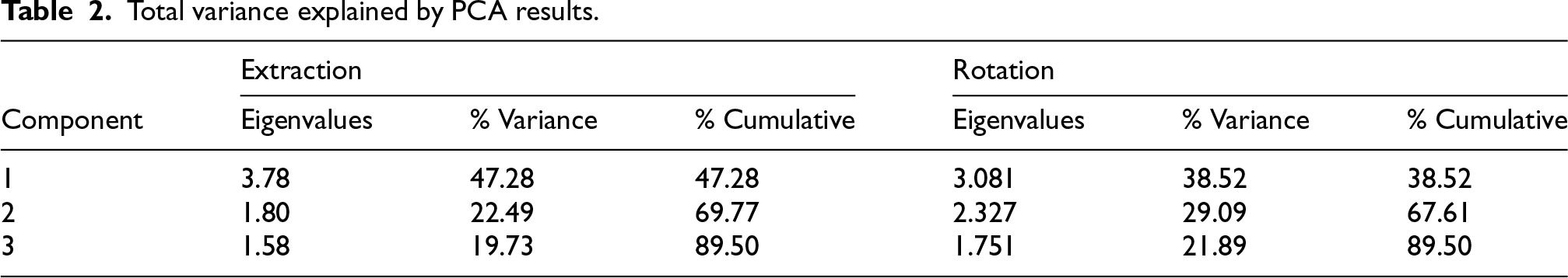
The optimal number of components in this research was determined based on eigenvalues, which assessed the significance of each component. The analysis identified three components with eigenvalues greater than 1.0, collectively explaining 89.50% of the total variance, which was sufficient to capture the variation among the original set of eight indicators (Table 2).

Table 2.
Total variance explained by PCA results.

Extraction Rotation

Component Eigenvalues % Variance % Cumulative Eigenvalues % Variance % Cumulative

1 3.78 47.28 47.28 3.081 38.52 38.52

2 1.80 22.49 69.77 2.327 29.09 67.61

3 1.58 19.73 89.50 1.751 21.89 89.50

	Extraction	Rotation
1	3.78	47.28	47.28	3.081	38.52	38.52
2	1.80	22.49	69.77	2.327	29.09	67.61
3	1.58	19.73	89.50	1.751	21.89	89.50

3.3.4 Interpretation and validation

For a more meaningful pattern and uncorrelated components, the study applied an orthogonal VARIMAX rotation to redistribute variance among the components, enhancing interpretability. The results showed no cross-loadings (high loading over 0.60 more than one component), meaning an optimal structure exists (Table 2).

After achieving a satisfactory pattern, the economic interpretation focused on loadings in a given component driving the variation among the potential leading indicators to help identify the underlying components and provide insights into economic significance.

The first component could be represented as the “Economic Activity Driver” since it captures the key factors of economic engagement of both production output and business sentiment that contribute to economic growth. The four indicators in this component affected the economy and were mutually correlated positively. The VAPI measures the efficiency and scale of economic production. The Consumption of Fixed Capital (CFC) accounts for the depreciation of capital goods, providing insight into the sustainability of economic activity over time–CFC tends to increase when production grows because more capital goods are being used or replaced. In the meantime, the BSI for both present (BSI) and future expectations (BSI3 M) provides insight into the confidence levels of businesses that drive economic growth.

The second component could be “Economic Investment Trend” since it reflects the broader trends of investment in both physical and financial activities of Domestic Machinery Sales (DMS) and Market Capitalization (MCAP). These two indicators were mutually pro-cyclical conformity and also with GDP; hence, the more this component there is, the more economic expansion there will be. As for physical investment, DMS indicates investments in capital goods and production capacity, whereas MCAP represents the value of assets in the financial markets. This component captures the investment landscape view for both physical (machinery) and financial (market-based) investments that drive productivity and economic growth.

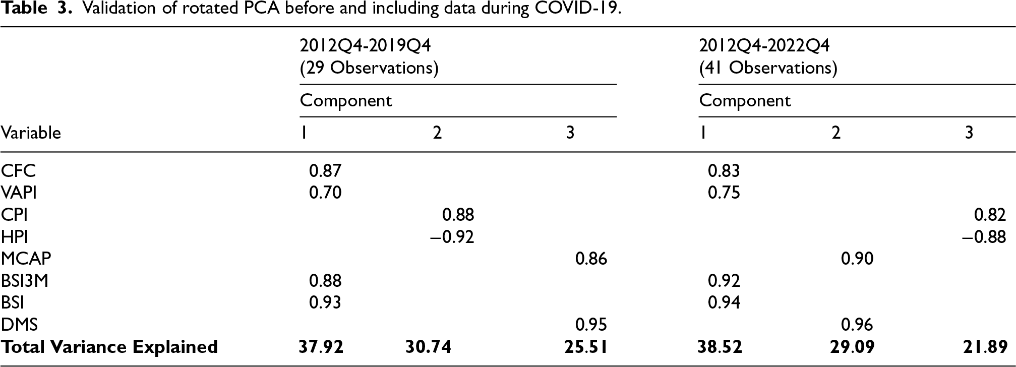
The third component could capture the underlying “Economic Price Pressure,” which includes the two indicators related to pricing– Consumer Price Index (CPI) and Housing Price Index (HPI). They exhibited a negative mutual correlation. The loading value for CPI was positive, while HPI was negative. This result aligned with cross-correlation analysis in that these indicators had opposite relationships with GDP: CPI correlated negatively, while HPI correlated positively, consistent with previous findings.^40–42 As for an economic explanation, increasing CPI could raise the cost of living, signal inflation, and lead to higher interest rates, negatively affecting the economy. Meanwhile, decreasing HPI might lower household wealth and dampen consumer confidence, reducing economic activity.^17,43

As for validating the PCA results, the research compared the results of data subsets. According to Hair, Black,²⁶ PCA typically requires at least five observations per variable. Since the research identified eight potential leading indicators, there should be at least 40 observations for the analysis. However, the available data length was limited, especially CFC, which was first available in 2012Q4. Thus, the study compared two subsets–before and including the last critical event of the COVID-19 epidemic: one covering 29 observations from 2012Q4 to 2019Q4 (fewer than five observations per variable) and another with 41 observations from 2012Q4 to 2022Q4. The comparison revealed that prior to COVID-19, the “ Economic Price Pressures” accounted for more explained variance than the “Economic Investment Trends” and vice versa for the data set covering the pandemic period. Despite these variations, the PCA results demonstrated consistency in the structure and signs of loadings across both subsets, suggesting stability (Table 3).

Table 3.
Validation of rotated PCA before and including data during COVID-19.

2012Q4-2019Q4 2012Q4-2022Q4

(29 Observations) (41 Observations)

Component Component

Variable 1 2 3 1 2 3

CFC 0.87 0.83

VAPI 0.70 0.75

CPI 0.88 0.82

HPI −0.92 −0.88

MCAP 0.86 0.90

BSI3M 0.88 0.92

BSI 0.93 0.94

DMS 0.95 0.96

Total Variance Explained 37.92 30.74 25.51 38.52 29.09 21.89

3.3.5 Additional uses of PCA to construct CLIs

To better understand the interrelationships among leading indicators and enhance the predictive power of individual series, this study employed PCA for data reduction to construct CLIs for each component dimension.

Many studies used unequal weight for constructing CLI based on the loading values, inferring that the contribution of each leading indicator is proportional to the magnitude of its loading in the PCA.^13,14 However, the majority of CLIs are constructed using equal weights.^19,35 Additionally, the loadings in this study were not substantially diverse; therefore, an equal-weighted approach was used for constructing the CLI. Note that if some indicators were unavailable for a given period, the study averaged only the available data to construct the CLI.

The CLIs for each component (CLI1, CLI2, and CLI3) were constructed using equal weights and based on the sign of the loadings shown in Table 1. Indicators with negative loadings were reverse-scaled before being incorporated into the CLIs. For CLI3, reversal scaling was necessary for HPI as it explicitly showed the negative loading sign. Since orthogonal rotation was used, the three CLIs were uncorrelated, each capturing unique aspects of the economic aspect. Additionally, a benchmark CLI, referred to as CLI4, was constructed using all eight indicators to compare with the three component-specific CLIs.

4. Empirical evaluation of CLIs

Those four CLIs were examined for their leading performance with the widely used techniques of cross-correlation and turning point analysis.^13,35

4.1 Conformity between CLIs and GDP

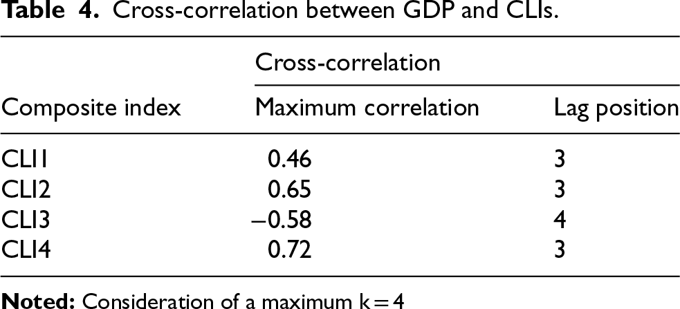
As for the conformity of a whole cycle leading ability, the CCF was applied to analyze each pair of GDP and CLI. Consideration of a maximum k at 4 revealed that CLIs were capable of leading GDP with the maximum cross-correlation over 0.40. CLI4 gained the highest maximum cross-correlation at 0.72, while CLI1 provided at 0.46 (Table 4). Although the size of the highest cross-correlation offers information on the relationship strength between the GDP and CLI, the size cannot be the only indicator used for identifying the best CLI.¹⁹ Therefore, the study evaluated CLIs’ turning point signal to GDP and real-time forecasting in the following section. As for the following sections in 4.2 and 4.3, since CLI3 had a negative maximum correlation, a counter-cyclical fluctuation with GDP, the study inversed its scale as CLI3R = 1-CLI3. Figure 1 depicts the conformity of a whole cycle leading ability to GDP of CLI1, CLI2, CLI3R, and CLI4.

Figure 1.

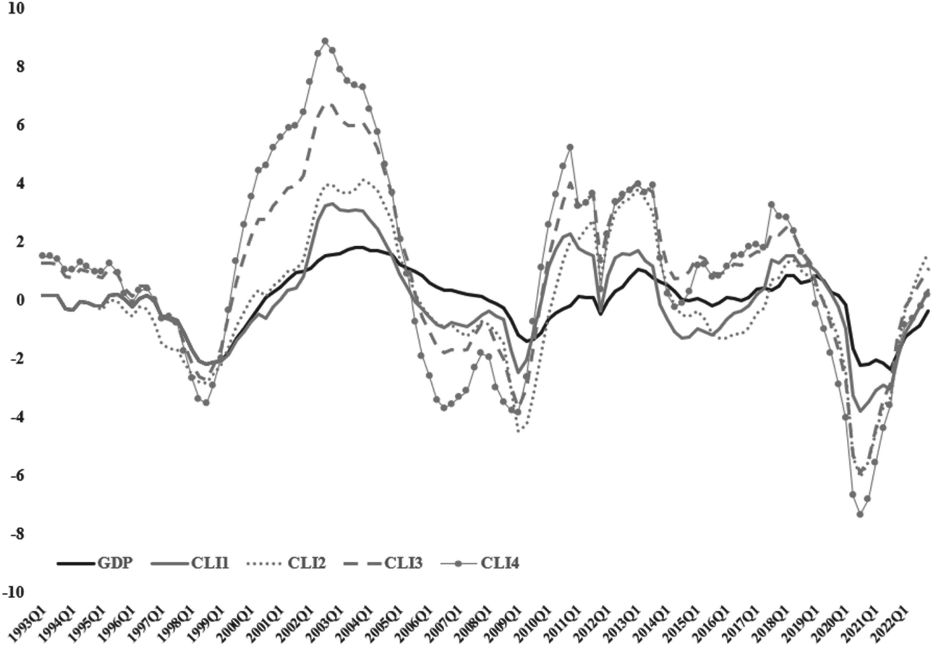
The cyclical movement of GDP, CLI1, CLI2, CLI3R, and CLI4.

Table 4.

Cross-correlation between GDP and CLIs.

	Cross-correlation
Composite index	Maximum correlation	Lag position
CLI1	0.46	3
CLI2	0.65	3
CLI3	−0.58	4
CLI4	0.72	3

Noted: Consideration of a maximum k = 4

4.2 CLIs performance in signaling early turning points of GDP

Further evaluation of the CLIs focused on their ability to signal turning points, as this research aimed to construct CLIs for Thailand's economic activities with an emphasis on providing early signals of business cycle turning points. The four CLIs were examined for their cyclical behavior to the turning points of GDP.

4.2.1 Evaluation of cyclical behavior of GDP

Turning point analysis following Bry and Boschan⁴⁴ was employed to evaluate the peaks and troughs of Thailand's economic cycle. As suggested by Harding and Pagan,⁴⁵ who extended the BryBoschan algorithm, the study identified the criteria for the minimum range of phase (the distance between a peak and a trough or vice versa) and the cycle (the distance between two consecutive peaks or troughs) for two and five quarters, respectively; additionally, peaks and troughs must alternate.

The initial results displayed 12 turning points with six peaks and six troughs. However, this study discarded five points for the following reasons. The first three turning points were ignored owing to the DoneHP, which was related to OneHP that could distort the early detection of turning points.⁴⁶ The study also excluded the turning points of the natural disaster, the severe flood in Thailand in 2011. However, the COVID-19 epidemic was retained in the analysis as the World Health Organization (WHO) declared the situation a global pandemic in March 2020. During the epidemic, the number of infections surged rapidly, with many resulting in deaths. In response, governments implemented national lockdowns, significantly impacting the business cycle.^10,47 (Figure 2).

Figure 2.

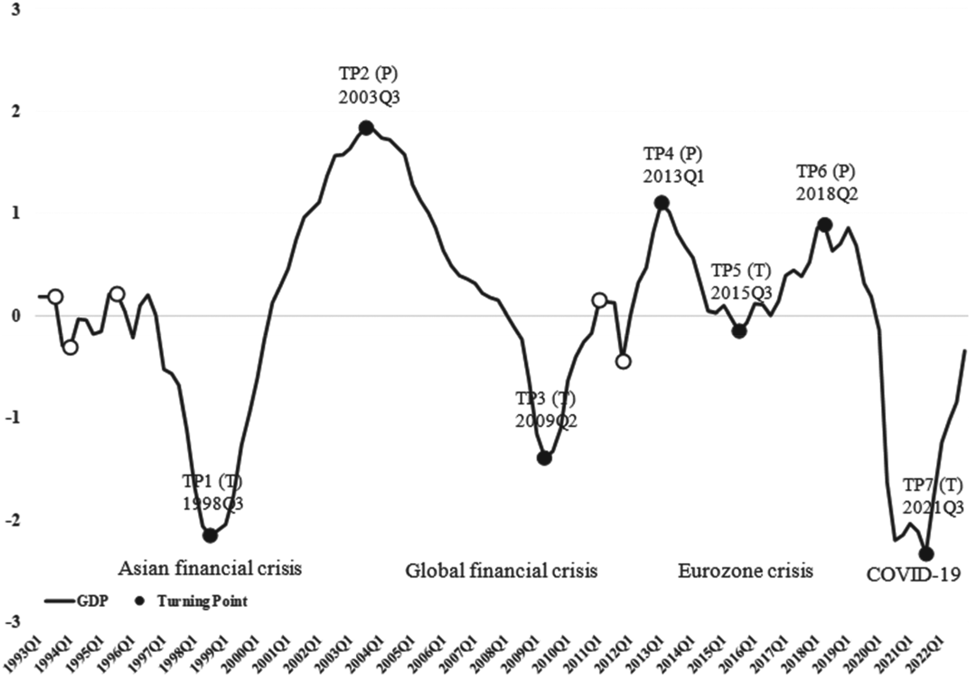
The turning point analysis of GDP during 1993Q1-2022Q4.

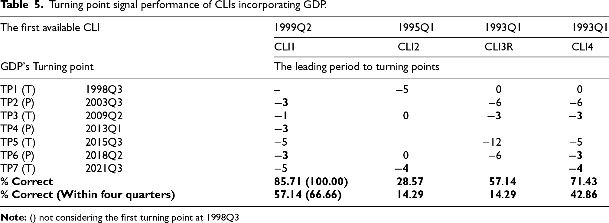
4.2.2 Evaluation of CLIs for signaling turning points in GDP

The evaluation of CLIs’ ability to signal turning points in GDP was based on each CLI's latest turning point, incorporating seven turning points of GDP. CLI1 demonstrated the best performance, achieving 85.71%. However, it could not signal the first turning point due to its limited data availability, as its first available component was in 1999Q2. If the first turning point in 1998Q3 was excluded, the study could infer that CLI1 would have signaled all turning points correctly (100%), followed by CLI4, CLI3R, and CLI2. When considering only early signals within four quarters (leading between 1 to 4 periods), CLI1 also outperformed that correctly identified 57.14% of the turning points (or 66.66% when excluding the first turning point out of consideration), followed by CLI4, while CLI2 and CLI3R performing identical (Table 5).

Table 5.
Turning point signal performance of CLIs incorporating GDP.

The first available CLI 1999Q2 1995Q1 1993Q1 1993Q1

CLI1 CLI2 CLI3R CLI4

GDP's Turning point The leading period to turning points

TP1 (T) 1998Q3 – −5 0 0

TP2 (P) 2003Q3 −3 −6 −6

TP3 (T) 2009Q2 −1 0 −3 −3

TP4 (P) 2013Q1 −3

TP5 (T) 2015Q3 −5 −12 −5

TP6 (P) 2018Q2 −3 0 −6 −3

TP7 (T) 2021Q3 −5 −4 −4

% Correct 85.71 (100.00) 28.57 57.14 71.43

% Correct (Within four quarters) 57.14 (66.66) 14.29 14.29 42.86

The first available CLI	1999Q2	1995Q1	1993Q1	1993Q1
TP1 (T)	1998Q3	–	−5	0	0
TP2 (P)	2003Q3	−3		−6	−6
TP3 (T)	2009Q2	−1	0	−3	−3
TP4 (P)	2013Q1	−3
TP5 (T)	2015Q3	−5		−12	−5
TP6 (P)	2018Q2	−3	0	−6	−3
TP7 (T)	2021Q3	−5	−4		−4
% Correct	85.71 (100.00)	28.57	57.14	71.43
% Correct (Within four quarters)	57.14 (66.66)	14.29	14.29	42.86

Note: () not considering the first turning point at 1998Q3

4.3 Evaluation of real-time forecasting

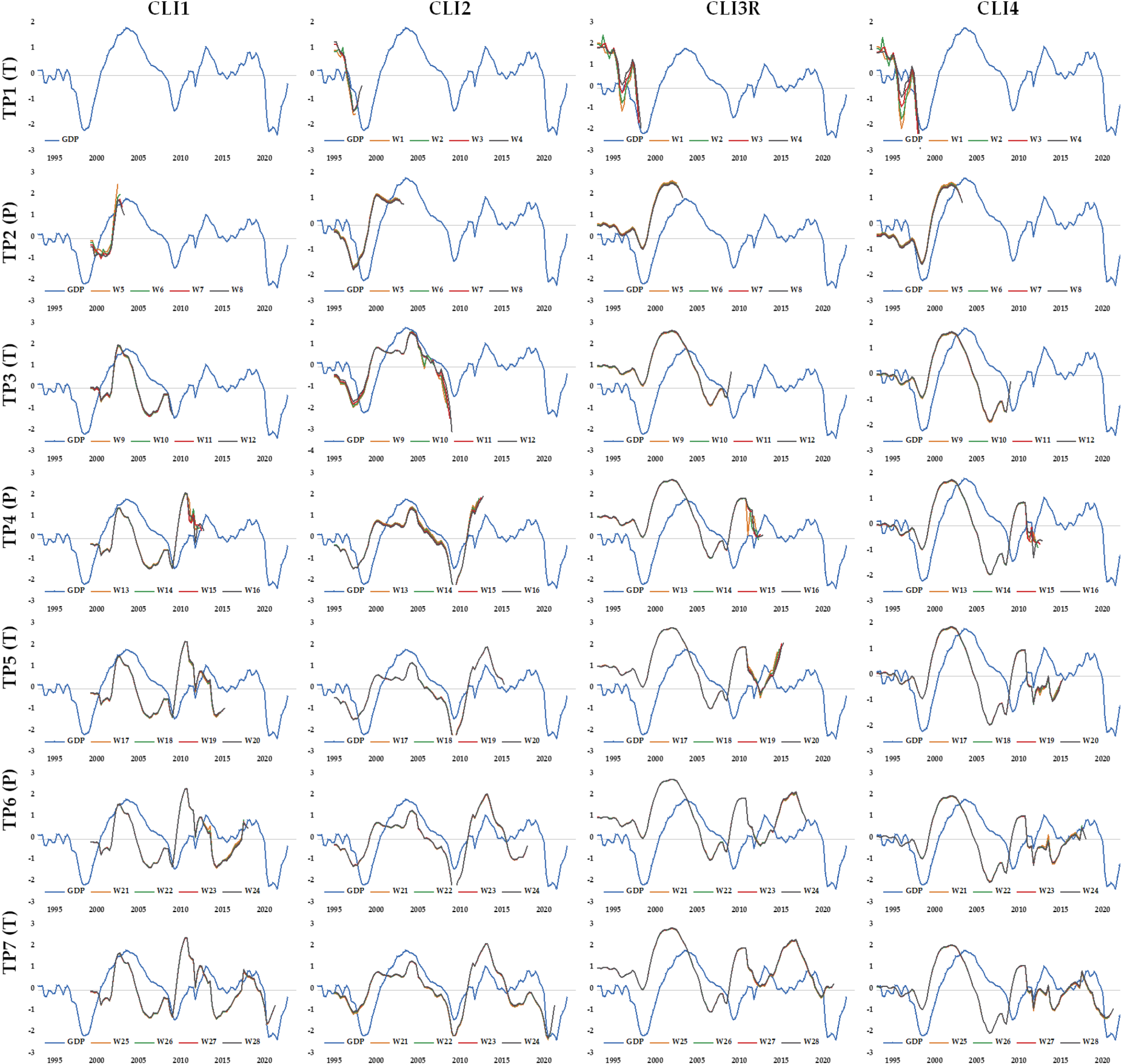
The study applied a pseudo-real-time analysis, mimicking real-time conditions, as vintage data from each point in time was not accessible. This real-time analysis was experimented with expanding data windows (W) to examine the cyclical behavior of the CLIs in relation to GDP cycles. Each window contained data up to the turning points, as available prior to those points.

4.3.1 Evaluation of real-time turning point signal performance

The 28 windows corresponded to the seven specified turning points of GDP, with four windows for each turning point. Each window contained data from 1 to 4 quarters prior to the turning point. For instance, the first turning point of GDP in the analysis occurred in 1998Q3; therefore, the last dates for the first to fourth windows were 1997Q3, 1997Q4, 1998Q1, and 1998Q2, respectively. Each window was expected to start at 1993Q1; however, some indicators might have started later than 1993Q1 due to data availability (Table 1). Recursively re-estimating four CLIs was estimated for each window (including filtering data), and then the turning point of CLIs was identified by the Bry-Boschan algorithm.

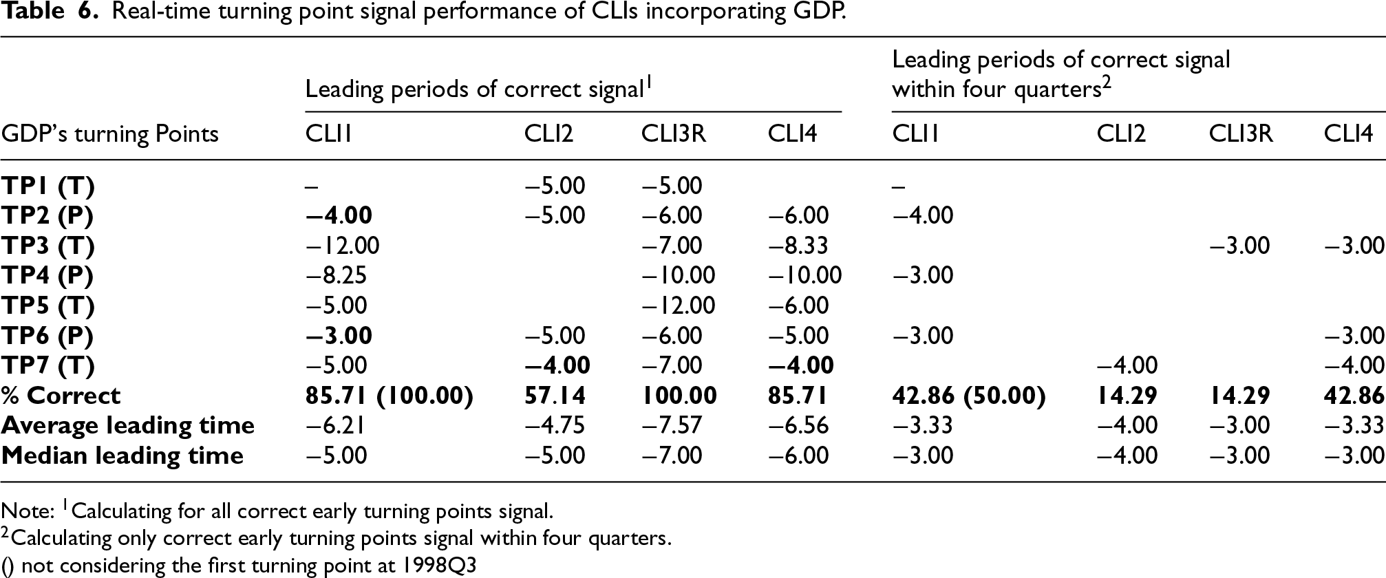
Real-time turning point performance focusing on the last CLI's turning point of the data window will be considered a correct signal if the CLI signaling matches the GDP turning point target. As for real-time turning point forecasting results (Table 6, Figure 3), CLI3R and CLI1 signaled early for all turning points (CLI3R for seven and CLI1 for six turning points, as mentioned earlier), followed by CLI4 and CLI2. However, when considering only early signals within four quarters, no single CLI could signal for all turning points, with each CLI exhibiting its own characteristics. Generally, peaks require more careful examination¹⁴; CLI1 performed well in signaling all peaks but failed to signal troughs early within four quarters. In contrast, CLI2 and CLI3R complemented each other by predicting troughs at different turning points. Regarding CLI4, it was able to forecast one peak and two troughs.

Figure 3.

Real-time turning point signal performance of CLIs incorporating GDP.

Table 6.

Real-time turning point signal performance of CLIs incorporating GDP.

	Leading periods of correct signal¹				Leading periods of correct signal within four quarters²
GDP's turning Points	CLI1	CLI2	CLI3R	CLI4	CLI1	CLI2	CLI3R	CLI4
TP1 (T)	–	−5.00	−5.00		–
TP2 (P)	−4.00	−5.00	−6.00	−6.00	−4.00
TP3 (T)	−12.00		−7.00	−8.33			−3.00	−3.00
TP4 (P)	−8.25		−10.00	−10.00	−3.00
TP5 (T)	−5.00		−12.00	−6.00
TP6 (P)	−3.00	−5.00	−6.00	−5.00	−3.00			−3.00
TP7 (T)	−5.00	−4.00	−7.00	−4.00		−4.00		−4.00
% Correct	85.71 (100.00)	57.14	100.00	85.71	42.86 (50.00)	14.29	14.29	42.86
Average leading time	−6.21	−4.75	−7.57	−6.56	−3.33	−4.00	−3.00	−3.33
Median leading time	−5.00	−5.00	−7.00	−6.00	−3.00	−4.00	−3.00	−3.00

Note: ¹Calculating for all correct early turning points signal.

Calculating only correct early turning points signal within four quarters.

() not considering the first turning point at 1998Q3

At this point, the results inferred that including all leading indicators as CLI4 or using only the first component from PCA as CLI1 was not the optimal solution, as each had its own unique characteristics. Hence, the study suggests using all potential leading indicators but reducing their dimensionality from 8 indicators to 3 CLIs.

4.3.2 Evaluation of out-of-sample forecasting performance

As for evaluating the study's suggestion, using all potential leading indicators but reducing them to a smaller dimension (from 8 indicators to 3 CLIs) instead of using all of them in a single CLI (CLI4), the study estimated two regression models to assess their forecasting performance. Regarding the independent variables to forecast GDP, the first equation (EQ1) included CLI1, CLI2, and CLI3R, while the second equation (EQ2) used CLI4. The primary objective of this section was to compare two approaches: using multiple CLIs working together (CLI1, CLI2, and CLI3R) versus using all indicators in a single CLI (CLI4). The goal was not to identify the optimal forecasting equation. The lag for each CLI in the model was determined based on the position that produced the highest correlation from the cross-correlation analysis between the CLIs and GDP. At this stage, the statistical assumptions, such as normality, stationarity, and serial correlation, were not fully addressed. As for improving the models, further steps could include transforming the data or selecting the optimal lag length. Although the regression assumptions were not fully considered at this point, the forecasting models were still able to distinguish between these two approaches.¹³

\begin{matrix} \begin{aligned} E Q 1 : G D P_{t} & = β_{0} + β_{1} C L I 1_{t - 3} + β_{2} C L I 2_{t - 3} + β_{3} C L I 3 R_{t - 4} \\ + ε_{t} \end{aligned} \end{matrix}

(3)

\begin{matrix} E Q 2 : G D P_{t} = β_{0} + β_{1} C L I 4_{t - 3} + ε_{t} \end{matrix}

(4)

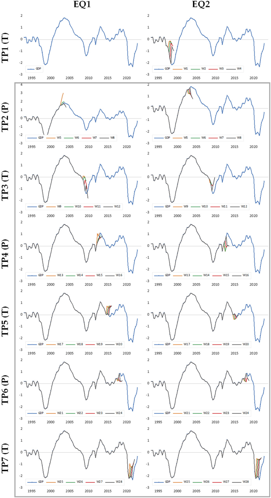
Although the regression equations forecasted the entire time series, this section focused on predicting each turning point. Therefore, the data windows from Section 4.3.1 were applied here. However, only 24 windows (W5 to W28, forecasting TP2 to TP7) were used, as the limitation of available data for estimating EQ1. For example, W5 to W8 aimed to forecast TP2 (the peak at 2003Q3); the last data points for estimating a regression equation of each window were 2002Q3, 2002Q4, 2003Q1, and 2003Q2, to forecast out-of-sample for three quarters: 2002Q4-2003Q2, 2003Q1-2003Q3, 2003Q2-2003Q4, and 2003Q3-2004Q1, respectively.

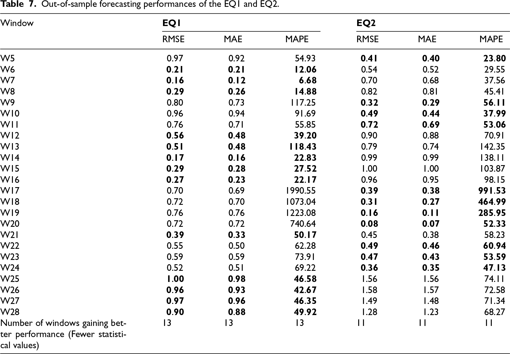
The out-of-sample forecasting results in Figure 4 depict that both EQ1 and EQ2 can signal the turning point. However, when evaluating the forecast error of each window using Root Mean Square Error (RMSE), Mean Absolute Error (MAE), and Mean Absolute Percentage Error (MAPE), the out-of-sample forecasting errors of 24 windows in Table 7 reveal that EQ1 outperformed EQ2. Specifically, EQ1 shows lower RMSE, MAE, and MAPE in 13 out of the 24 windows (54.17%), indicating that using CLIs together in EQ1 yielded better results than using all indicators in one CLI in EQ2 (45.83%). While the results did not reach a consensus, the majority of the evidence supported the previous evaluations.

Figure 4.

Out-of-sample forecasting performances of the EQ1 and EQ2.

Table 7.

Out-of-sample forecasting performances of the EQ1 and EQ2.

Window	EQ1			EQ2
	RMSE	MAE	MAPE	RMSE	MAE	MAPE
W5	0.97	0.92	54.93	0.41	0.40	23.80
W6	0.21	0.21	12.06	0.54	0.52	29.55
W7	0.16	0.12	6.68	0.70	0.68	37.56
W8	0.29	0.26	14.88	0.82	0.81	45.41
W9	0.80	0.73	117.25	0.32	0.29	56.11
W10	0.96	0.94	91.69	0.49	0.44	37.99
W11	0.76	0.71	55.85	0.72	0.69	53.06
W12	0.56	0.48	39.20	0.90	0.88	70.91
W13	0.51	0.48	118.43	0.79	0.74	142.35
W14	0.17	0.16	22.83	0.99	0.99	138.11
W15	0.29	0.28	27.52	1.00	1.00	103.87
W16	0.27	0.23	22.17	0.96	0.95	98.15
W17	0.70	0.69	1990.55	0.39	0.38	991.53
W18	0.72	0.70	1073.04	0.31	0.27	464.99
W19	0.76	0.76	1223.08	0.16	0.11	285.95
W20	0.72	0.72	740.64	0.08	0.07	52.33
W21	0.39	0.33	50.17	0.45	0.38	58.23
W22	0.55	0.50	62.28	0.49	0.46	60.94
W23	0.59	0.59	73.91	0.47	0.43	53.59
W24	0.52	0.51	69.22	0.36	0.35	47.13
W25	1.00	0.98	46.58	1.56	1.56	74.11
W26	0.96	0.93	42.67	1.58	1.57	72.58
W27	0.97	0.96	46.35	1.49	1.48	71.34
W28	0.90	0.88	49.92	1.28	1.23	68.27
Number of windows gaining better performance (Fewer statistical values)	13	13	13	11	11	11

5. Conclusions and final remarks

This research examined several official statistical data to identify leading indicators of Thailand's business cycle from 1993Q1 to 2022Q4. Based on Cross-correlation analysis and researcher judgment, eight potential leading indicators were identified for their ability to signal GDP fluctuations up to four quarters in advance. Principal Component Analysis (PCA) was then applied to reduce these indicators into smaller dimensions, which were constructed into three component-specific Composite Leading Indicators (CLI1, CLI2, and CLI3). Additionally, all eight indicators were combined into the fourth CLI (CLI4) as a benchmark for comparison.

The CCF once again assessed the overall cycle-leading capability of the CLIs to GDP. The results showed that most CLIs were pro-cyclical, except for CLI3, which exhibited a counter-cyclical pattern with GDP; thus, its scaling was reversed and renamed as CLI3R. In evaluating real-time turning point forecasting, CLI1 and CLI3R successfully identified all turning points. However, when focusing solely on early signals within a four-quarter, no single CLI could capture all turning points since each CLI had its own characteristics.

In this context, including all leading indicators in a single CLI (CLI4) or relying solely on the first component from PCA (CLI1) was not found to be the optimal approach. Instead, the study recommends using a smaller dimensionality, reducing the eight potential leading indicators into three distinct CLIs.This recommendation is supported by evidence from out-of-sample forecasting errors from regression models, using all eight leading indicators as independent variables in two versions: one using the three separate CLIs and another using a single CLI4. Although the results were not entirely conclusive, the majority of evidence favored the approach of using the three distinct CLIs, which provided better forecasting accuracy than aggregating all indicators into a single CLI (CLI4).

For policy implementation, combining too many indicators into a single composite index can obscure the specific drivers affecting overall outcomes, making it difficult to identify the target policy contributing to the positive result.⁴⁸ Thus, instead of combining the eight indicators into one or using each separately, the study recommends applying the three distinct CLIs together to offer a more precise analysis.

This approach enhances early warning capabilities for economic turning points by capturing key dimensions in a simplified framework, supporting more effective policy responses. As for the economic explanation of the three distinct CLIs, since economic peaks can potentially cause more severe damage than troughs, policymakers should emphasize CLI1. This component, labeled “Economic Activity Driver,” comprises the VAPI, Consumption of Fixed Capital (CFC), and the BSI for both present (BSI) and future expectations (BSI3 M). These indicators collectively capture the key aspects of economic engagement, encompassing both production output and business sentiment, which are critical for fostering economic growth. Meanwhile, policymakers should also monitor the remaining two CLIs. CLI2, constructed from DMS and Market Capitalization (MCAP), can be referred to as “Economic Investment Trend” since it captures the investment landscape for both physical (machinery) and financial (market-based) investments that drive productivity and economic growth. The final CLI, CLI3, comprises two pricing-related indicators—CPI and HPI. These indicators exhibit a negative mutual correlation, with HPI being reverse-scaled before constructing CLI3. As such, CLI3 reflects broader economic pressure from pricing as “Economic Price Pressure.” A rising CLI3 signals a combination of increasing cost of living (inflation) and declining household wealth, negatively impacting GDP and overall economic growth.

With the complementarity of these three CLIs, policymakers can calculate each CLI individually but monitor them collectively as “Economic Activity Driver,” “Economic Investment Trend,” and “Economic Price Pressure.” The advantage of separately calculating each CLI lies in its simplicity and ease of construction, allowing for a more straightforward approach to analysis.

Although multivariate normality is not a strict requirement for PCA, its assumption enhances the robustness of interpretation. Deviations from normality, common in macroeconomic data, may impact the validity of patterns derived. Therefore, the results should be interpreted with caution. To address this limitation, the study validated the findings by comparing PCA results across data subsets to ensure pattern consistency.

For further research, while this study focused on uncovering dimensions of leading indicators for exploratory insights, future studies could extend this work by incorporating confirmatory techniques, such as Structural Equation Modeling (e.g., Partial Least Squares Structural Equation Modeling). Exploring alternative seasonal adjustment and cyclical extraction methods alongside the analysis may also enhance the robustness and interpretability of results.

Footnotes

Acknowledgments

I sincerely thank the editor and reviewers for their constructive comments and valuable feedback, which have significantly improved the quality and clarity of my manuscript. I would also like to express my gratitude to the funding by the National Science, Research and Innovation Fund, Thailand Science Research and Innovation (TSRI), through Rajamangala University of Technology Thanyaburi (FRB66E0643O.1) (Grant No.: FRB660012/0168).

ORCID iD

Jeerawadee Pumjaroen

Funding

This research was supported by the National Science, Research and Innovation Fund, Thailand Science Research and Innovation (TSRI), through Rajamangala University of Technology Thanyaburi Thanyaburi (FRB66E0643O.1) (Grant No.: FRB660012/0168).

Declaration of conflicting interests

The author declared no potential conflicts of interest with respect to the research, authorship, and/or publication of this article.

Appendix A

Table A1.

The comparison results of the Cross-Correlation Function with the non-parametric measures of Spearman's rho and Kendall's tau.

	k	CFC	VAPI	CPI	HPI	MCAP	BSI3M	BSI	DMS
	−4	−0.27	−0.08	0.00	−0.04	0.07	−0.16	−0.20	−0.02
	−3	−0.12	0.04	−0.06	0.02	0.20	−0.05	−0.10	0.08
	−2	0.02	0.19	−0.12	0.09	0.33	0.07	0.02	0.18
	−1	0.12	0.36	−0.19	0.16	0.45	0.20	0.15	0.30
	0	0.22	0.53	−0.25	0.24	0.54	0.32	0.28	0.40
	1	0.33	0.57	−0.31	0.33	0.61	0.41	0.36	0.46
	2	0.41	0.56	−0.37	0.43	0.64	0.45	0.40	0.48
Cross-correlation	3	0.42	0.51	−0.42	0.52	0.63	0.47	0.42	0.49
	4	0.41	0.39	−0.47	0.59	0.60	0.45	0.41	0.49
	−4	−0.54	−0.06	0.06	−0.17	0.14	−0.18	−0.19	−0.03
	−3	−0.30	0.10	0.00	−0.12	0.25	−0.06	−0.08	0.06
	−2	−0.05	0.31	−0.07	−0.07	0.34	0.06	0.03	0.15
	−1	0.12	0.49	−0.14	−0.03	0.43	0.17	0.14	0.24
	0	0.25	0.65	−0.22	0.02	0.51	0.28	0.24	0.31
	1	0.43	0.69	−0.31	0.10	0.57	0.37	0.34	0.38
	2	0.59	0.64	−0.39	0.19	0.61	0.44	0.42	0.44
Spearman's rho	3	0.65	0.57	−0.47	0.30	0.63	0.48	0.47	0.49
	4	0.65	0.44	−0.55	0.40	0.64	0.50	0.49	0.53
	−4	−0.38	−0.05	0.04	−0.12	0.11	−0.13	−0.13	−0.01
	−3	−0.22	0.05	0.00	−0.07	0.19	−0.05	−0.06	0.04
	−2	−0.05	0.20	−0.04	−0.04	0.25	0.04	0.02	0.10
	−1	0.06	0.35	−0.09	−0.02	0.31	0.12	0.11	0.16
	0	0.15	0.50	−0.15	−0.01	0.36	0.20	0.18	0.20
	1	0.27	0.52	−0.21	0.04	0.41	0.26	0.26	0.24
	2	0.40	0.47	−0.27	0.11	0.43	0.32	0.32	0.29
Kendall's tau	3	0.46	0.39	−0.32	0.19	0.45	0.35	0.35	0.33
	4	0.44	0.31	−0.37	0.27	0.46	0.36	0.36	0.36

References

Burns

Mitchell

. Measuring business cycles. New York: National Bureau of Economic Research, 1946.

Mazzi

Scocco

. Bussiness cycles analysis and related software applications. Luxemburgo: Office for Official Publications of the Europeans Communities Recuperado el, 2003, p. 26.

Calderón

Fuentes

. Characterizing the business cycles of emerging economies. World Bank Policy Research Working Paper. 2010(5343).

Gatfaoui

Girardin

. Comovement of Chinese provincial business cycles. Econ Model 2015; 44: 294–306.

Mintz

. Dating postwar business cycles: Methods and their application to Western Germany. New York: NBER Books, 1969, pp. 1950–1967.

Padilla

Quintero Otero

. Regional business cycles in emerging economies: a review of the literature. Int J Emerg Mark 2023; 18: 5217–5237.

Pumjaroen

Sethapramote

. Evaluating the robustness and implementing double one-sided Hodrick-Prescott for cycle extraction. ABAC J 2023; 43: 143–160.

Pholphirul

Rukumnuaykit

. The real estate cycle and real business cycle: evidence from Thailand. Pac Rim Prop Res J 2009; 15: 145–165.

Mitchell

Burns

. Statistical indicators of cyclical revivals. Statistical indicators of cyclical revivals. New York: NBER, 1938, pp. 1–12.

10.

Ruggeri Cannata

. The Eurostat business cycle clock: a complete overview of the tool. Stat J IAOS 2021; 37: 309–323.

11.

Stock

Watson

. New indexes of coincident and leading economic indicators. NBER Macroecon Ann 1989; 4: 351–394.

12.

Stock

Watson

. Forecasting using principal components from a large number of predictors. J Am Stat Assoc 2002; 97: 1167–1179.

13.

Levanon

Manini

J-C

Ozyildirim

, et al. Using financial indicators to predict turning points in the business cycle: the case of the leading economic index for the United States. Int J Forecast 2015; 31: 426–445.

14.

Atabek

Cosar

Sahinöz

. A new composite leading indicator for Turkish economic activity. Emerg Markets Fin Trade 2005; 41: 45–64.

15.

Wongwachara

Jindarak

Nookhwun

, et al. Integrating monetary policy and financial stability: a new framework. Thailand: Puey Ungphakorn Institute for Economic Research, 2018.

16.

Sethapramote

. Synchronization of business cycles and economic policy linkages in ASEAN. J Asian Econ 2015; 39: 126–136.

17.

Bank of Thailand. Leading economic index and components: Bank of Thailand, https://app.bot.or.th/BTWS_STAT/statistics/BOTWEBSTAT.aspx?reportID=887&language=ENG.

18.

Bilan

Gavurova

Stanisław

, et al. The composite coincident indicator (CCI) for business cycles. Acta Polytech Hung 2017; 14: 71–90.

19.

Gyomai

Guidetti

. OECD System of Composite Leading Indicators. 2012.

20.

Pumjaroen

Vichitthamaros

Sethapramote

. Forecasting economic cycle with a structural equation model: evidence from Thailand. Int J Econ Financ Issues 2020; 10: 47–57.

21.

Rose

Spiegel

. International financial remoteness and macroeconomic volatility. J Dev Econ 2009; 89: 250–257.

22.

Frankel

Saravelos

. Are leading indicators of financial crises useful for assessing country vulnerability? Evidence from the 2008-09 global crisis. National bureau of economic research; 2010. Report No.: 0898-2937.

23.

Kaminsky

Lizondo

Reinhart

. Leading indicators of currency crises. IMF Staff Papers 1998; 45: 1–48.

24.

Kaminsky

Reinhart

. The twin crises: the causes of banking and balance-of-payments problems. Am Econ Rev 1999; 89: 473–500.

25.

Babecký

Havranek

Matějů

, et al. Early Warning Indicators of economic crises: evidence from a panel of 40 Developed countries. Czech National Bank Working Paper. 2011;Series 8.

26.

Hair

Black

Babin

, et al. Multivariate data analysis: Pearson new international edition. Essex: Pearson Education Limited, 2014;1.

27.

Chauvet

Potter

. Coincident and leading indicators of the stock market. J Empir Fin 2000; 7: 87–111.

28.

Holmes

Shamsuddin

. Evaluation of alternative leading indicators of British Columbia industrial employment. Int J Forecast 1993; 9: 77–83.

29.

Hodrick

Prescott

. Post-war US business cycles: an empirical investigation. Northwestern University. Center for Mathematical Studies in Economics and Management Science, Discussion Papers. 1981;451.

30.

Hodrick

Prescott

. Postwar US business cycles: an empirical investigation. J Money Credit Bank 1997; 29: 1–16. doi:https://doi.org/10.2307/2953682

31.

Benes

N'Diaye

. A multivariate filter for measuring potential output and the nairu application to the Czech republic. IMF Working Papers. 2004.

32.

Schlicht

. Estimating the smoothing parameter in the so-called Hodrick-Prescott filter. J Jpn Stat Soc 2005; 35: 99–119.

33.

OECD. Composite leading indicator. In: (OECD) OfEC-oaD, editor. 2023.

34.

Hamilton

. Why you should never use the Hodrick-Prescott filter. Rev Econ Stat 2018; 100: 831–843.

35.

Tule

Ajilore

Ebuh

. A composite index of leading indicators of unemployment in Nigeria. J Afr Bus 2016; 17: 87–105.

36.

Fiorentini

Planas

. Busy program user manual. Joint Research Centre of European Commission Document. 2003.

37.

Mohanty

Singh

Jain

. Business cycles and leading indicators of industrial activity in India. 2003.

38.

Jawadi

Ameur

Bigou

, et al.

Does the real business cycle help forecast the financial cycle?

Comput Econ 2022; 60: 1529–1546.

39.

Forni

Hallin

Lippi

, et al. The generalized dynamic factor model: one-sided estimation and forecasting. J Am Stat Assoc 2005; 100: 830–840.

40.

Akinsola

Odhiambo

. Inflation and economic growth: A review of the international literature. 2017.

41.

Alexander

WRJ

. Inflation and economic growth: evidence from a growth equation. Appl Econ 1997; 29: 233–238.

42.

Vinayagathasan

. Inflation and economic growth: a dynamic panel threshold analysis for Asian economies. J Asian Econ 2013; 26: 31–41.

43.

Aizenman

Jinjarak

Zheng

. Housing bubbles, economic growth, and institutions. Open Econ Rev 2019; 30: 655–674.

44.

Bry

Boschan

. Front matter to “Cyclical Analysis of Time Series: Selected Procedures and Computer Programs”. Cyclical analysis of time series: Selected procedures and computer programs: NBEr, 1971, pp. 13–2.

45.

Harding

Pagan

. Dissecting the cycle: a methodological investigation. J Monet Econ 2002; 49: 365–381.

46.

Kaiser

Maravall

Kaiser

, et al. Some basic limitations of the Hodrick-Prescott filter. Measuring business cycles in economic time series. 2001, pp. 87–115.

47.

Kufel

Błażejowski

. Do COVID-19 lock-downs affect business cycle? Analysis using energy consumption cycle clock for selected European countries. Energies 2022; 15: 340.

48.

Gennari

Navarro

. The challenge of measuring agricultural sustainability in all its dimensions. J Sustain Res 2019; 1: e190013.

	Extraction			Rotation
Component	Eigenvalues	% Variance	% Cumulative	Eigenvalues	% Variance	% Cumulative
1	3.78	47.28	47.28	3.081	38.52	38.52
2	1.80	22.49	69.77	2.327	29.09	67.61
3	1.58	19.73	89.50	1.751	21.89	89.50

	2012Q4-2019Q4			2012Q4-2022Q4
	(29 Observations)			(41 Observations)
	Component			Component
Variable	1	2	3	1	2	3
CFC	0.87			0.83
VAPI	0.70			0.75
CPI		0.88				0.82
HPI		−0.92				−0.88
MCAP			0.86		0.90
BSI3M	0.88			0.92
BSI	0.93			0.94
DMS			0.95		0.96
Total Variance Explained	37.92	30.74	25.51	38.52	29.09	21.89

Conceptualizing economic leading indicators for early warning of Thailand's business cycle turning points

Abstract

Keywords

1. Introduction

2. Background

2.1 Reference series

2.2 Potential leading indicators

2.3 Composite leading index

2.4 Principal component analysis

3.1 Data preparation

3.2 Identification of potential leading indicators

3.3.1 PCA objectives

3.3.2 Statistical assumptions in PCA

3.3.3 Principal components assessment

Table 2. Total variance explained by PCA results. Extraction Rotation Component Eigenvalues % Variance % Cumulative Eigenvalues % Variance % Cumulative 1 3.78 47.28 47.28 3.081 38.52 38.52 2 1.80 22.49 69.77 2.327 29.09 67.61 3 1.58 19.73 89.50 1.751 21.89 89.50

4. Empirical evaluation of CLIs

4.1 Conformity between CLIs and GDP

4.2.1 Evaluation of cyclical behavior of GDP

4.3.1 Evaluation of real-time turning point signal performance

Footnotes

Acknowledgments

ORCID iD

Funding

Declaration of conflicting interests

Appendix A

References

Table 2.
Total variance explained by PCA results.

Extraction Rotation

Component Eigenvalues % Variance % Cumulative Eigenvalues % Variance % Cumulative

1 3.78 47.28 47.28 3.081 38.52 38.52

2 1.80 22.49 69.77 2.327 29.09 67.61

3 1.58 19.73 89.50 1.751 21.89 89.50