
Abstract
Paddy data is essential for policymakers to formulate Indonesia's national food security strategies, especially regarding harvested area. Currently, estimates are generated monthly using ground truth data from sampled locations through the Area Sampling Frames (ASF) process. However, the high cost and various field obstacles highlight the need for alternative methods. Satellite Imagery Time Series (SITS) data, mainly Sentinel-1 historical imagery, offers a promising alternative for detecting phenological stages. However, SITS data require machine learning modeling—for example, XGBoost—which has proven successful in several classification tasks. This study presents an alternative approach in West Java province, a major region for paddy production. The workflow includes preliminary analysis, data preprocessing, region-specific modelling, prediction, and estimation. Most regional clusters demonstrate high accuracy in classifying phenological stages, and harvested area patterns closely align with official statistics, demonstrating the effectiveness and potential of this approach.
Introduction
Paddy data is essential for policymakers in formulating national food security strategies, particularly in Indonesia. Accurate and timely paddy data relies on a well-designed data collection process that emphasizes the adoption of cutting-edge and cost-effective approaches. The critical importance of modernizing agricultural data systems is underscored by the National Long-Term Development Plan 2025–2045, which highlights the transformation of data collection in all sectors, including paddy production. 1 At present, Statistics Indonesia (BPS) estimates paddy production through two integrated primary surveys: the Area Sampling Frame (ASF) for determining harvested area and the Crop Cutting Survey for assessing productivity. However, the ASF methodology employs costly monthly ground-truthing to capture phenological stages, alongside several persistent challenges such as field inaccessibility due to remoteness, respondent non-response, and increased surveyor burden. 2
Alternatively, satellite imagery offers an efficient solution for estimating phenological stages without the need for extensive ground-truthing, enabling cost-effective, accurate, and timely calculation of harvested areas.3,4 Sentinel-1, a radar-based satellite, is particularly effective for large-scale agricultural monitoring because it can penetrate cloud cover, which is a significant advantage in Indonesia's frequently overcast conditions. 5 However, despite these advantages, relying solely on satellite imagery may not always provide the most reliable accuracy for phenological stage detection. 4 To achieve robust results, satellite data should be processed using cutting-edge methods such as machine learning; algorithms like XGBoost are particularly well-suited for classifying complex crop growth stages from satellite observations due to their excellent performance in multiclass classification tasks.6–8
This study aims to demonstrate the approach by implementing a systematic machine learning workflow focused on West Java, Indonesia—a pivotal region that accounted for about 30% of the country's total paddy production in 2022. The structure of this paper is as follows: the first section introduces the research context; the second describes the datasets used; the third explains the stepwise machine learning workflow; the fourth presents results and key insights; and the final section offers conclusions and recommendations.
Data
Satellite imagery time series
This analysis utilizes Satellite Imagery Time Series (SITS) data derived from historical Sentinel-1 imagery, obtained via the Alaska Satellite Facility (ASF) API for the period 2021–2023, at a biweekly temporal resolution. 9 Instead of the satellite image in one time, the longitudinal data of satellite image, which is SITS, is chosen to enhance the modelling of temporal trends. 10 To ensure each image quality, standard preprocessing steps—such as orbit file correction, thermal noise and border noise removal, radiometric calibration, speckle filtering, terrain correction, and mosaicking—is applied.11,12 All preprocessing procedures are conducted on an in-house server using the ESA-SNAP Python API, producing a time series of Sentinel-1 imagery focused on the VH-band, with a 20-meter spatial resolution. 11 After preprocessing, integration between Sentinel-1 imagery data and ASF field observations for the period February 2022–December 2023 is performed by spatial join techniques. Field observations are collected from 300 m × 300 m plots, each subdivided into nine 100 m × 100 m sub-grids. The corresponding time series segments are illustrated in Figure 1, where the yellow shaded region represents the final 12 weeks (± 90 days), corresponding to the most recent paddy cultivation period.
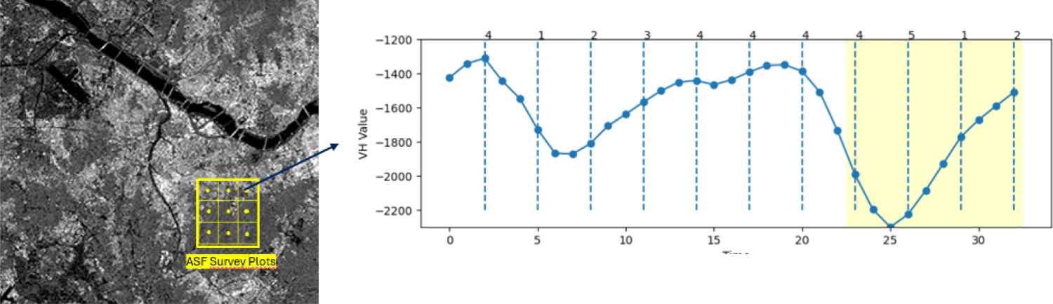
The ASF plot and sentinel 1 integration.
The ASF data, collected from monthly observations, is used as the ground truth label for the classification task. Phenological stages are recorded at the centroid of each sub-grid using geotagged points. Each monthly observation is matched (paired) with a set of SITS data of length 31, corresponding to the total images of Sentinel 1 collected biweekly in 1 years. However, several adjustments are made to stage labeling: non-paddy and no-vegetation categories are combined, and consecutive observations of land preparation and harvest are recategorized, as detailed in Table 1. For consecutive land preparation, only the last observation is designated as “land preparation,” while others are assigned to a newly created class (“bare-land”). Conversely, for consecutive harvest records, only the first observation is categorized as “harvest,” with the remainder also classified as “bare-land.”
Label (observation class) comparison from ASF and modified label in this study.
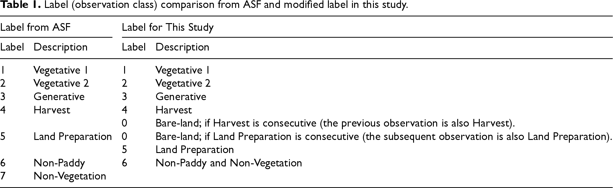
Label (observation class) comparison from ASF and modified label in this study.
Developing a robust machine learning workflow involves multiple operations, including preliminary analysis, data preprocessing, model development, prediction, and estimation. The following subsection describes the corresponding steps in each process.
Preliminary
As a preliminary step, represented in Figure 2, the regencies in focus regions undergo a clustering process based on agricultural and terrain characteristics, involving data as follows: previous total harvested area, previous total production area, number of paddy plantation cycles, elevation, evapotranspiration, and Land Surface Temperature (LST). The clustering process is designed to generate distinct groups of regencies that serve as the basis for machine learning modelling respective to the spatial constraints. Consequently, rather than employing a single global model, multiple models are developed, each tailored to the characteristics of its respective cluster. For this purpose, the Spatial ‘K'luster Analysis by Tree Edge Removal (SKATER) algorithm is implemented due to its competence in handling spatial clustering. 13
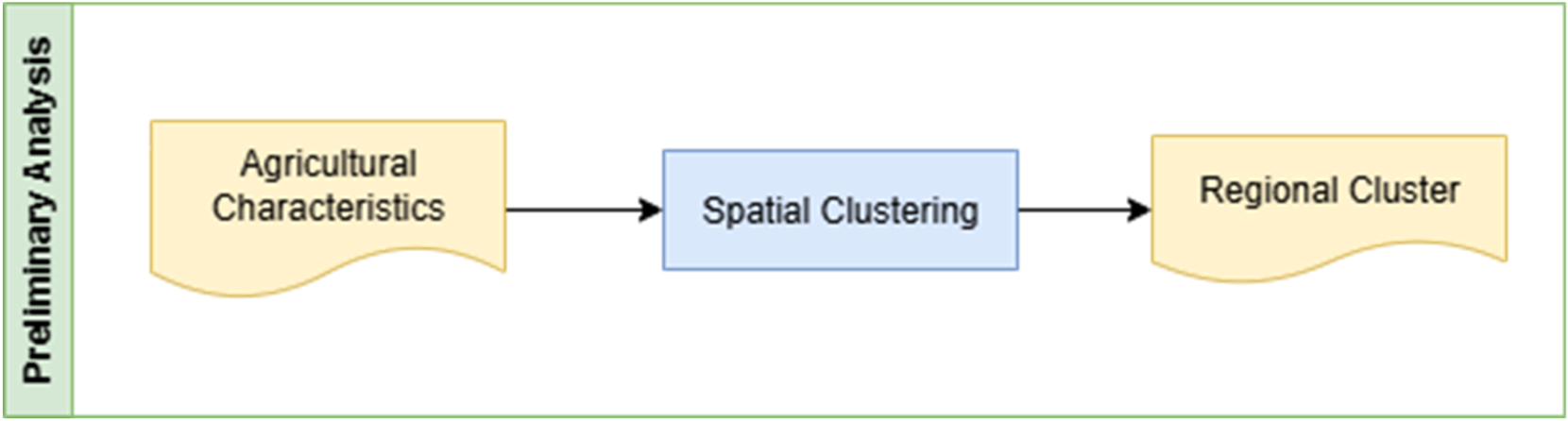
Preliminary analysis step.
After the first step is applied, three main preprocessing procedures are undertaken: imputing missing data, heterogeneity filtering, and noise filtering to ensure a well-representative training set.
The preprocessing step, depicted in Figure 3, begins by addressing missing values in the Sentinel data using the Whittaker-Eilers smoothing algorithm, which effectively fills gaps in time series data. 14 This ensures data continuity and reliability before further processing. Subsequently, to improve training dataset quality, grids with high heterogeneity are excluded using variance-based filtering. Sub-grids with excessive intra-cluster variability, measured by the variance of VH values over time, are removed if they exceed the third quartile (Q3) within each cluster. This criterion reflects mixed cropping practices commonly observed in Indonesia, which result in elevated VH variability within individual sub-grids. While this filtering step removes a non-negligible proportion of observations, it represents a deliberate trade-off between sample size and data homogeneity. By prioritizing more homogeneous agricultural patterns, the resulting training dataset improves model stability and robustness, at the cost of reduced representation of highly heterogeneous areas.
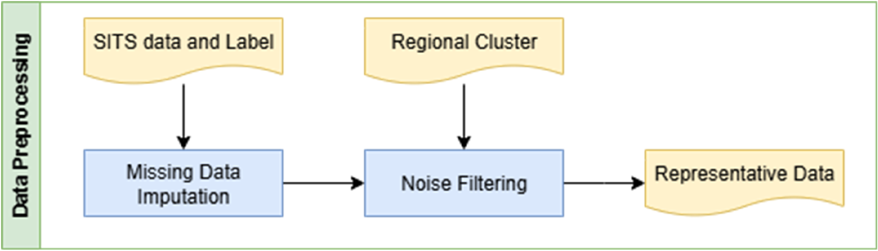
Data preprocessing step.
Lastly, Self-Organizing Map (SOM) filtering 15 is applied to noise filtering and enhance data representativeness. Each cluster is assigned 100 neurons, and neurons are selected based on the majority phenological stage. Observations most similar to these selected neurons are retained, while others are discarded.16,17 To introduce controlled randomness and reduce overfitting, 5% of the discarded observations are reintroduced into the training set.
Model development is conducted to several process, as depicted in Figure 4. The modelling process is applied in each regional cluster to improve the accuracy. At the first stage, the dataset is divided into two subsets: one containing all observations and another with 70% of the data. The smaller subset is then used to train the machine learning model, which is subsequently applied to predict the full dataset. This subset is further split into training and validation sets with a 70:30, while ensuring the distribution of paddy phenological stages remains representative. After thorough preprocessing of the training dataset, the modelling phase begins with hyperparameter tuning and cross-validation to optimize performance. 17 XGBoost is selected as the algorithm due to its robustness, efficiency, and ability to capture complex patterns. Since the task focuses on multiclass classification with imbalanced categories caused by the uneven distribution of paddy phenological stages, the imbalance is preserved to reflect real-world conditions.
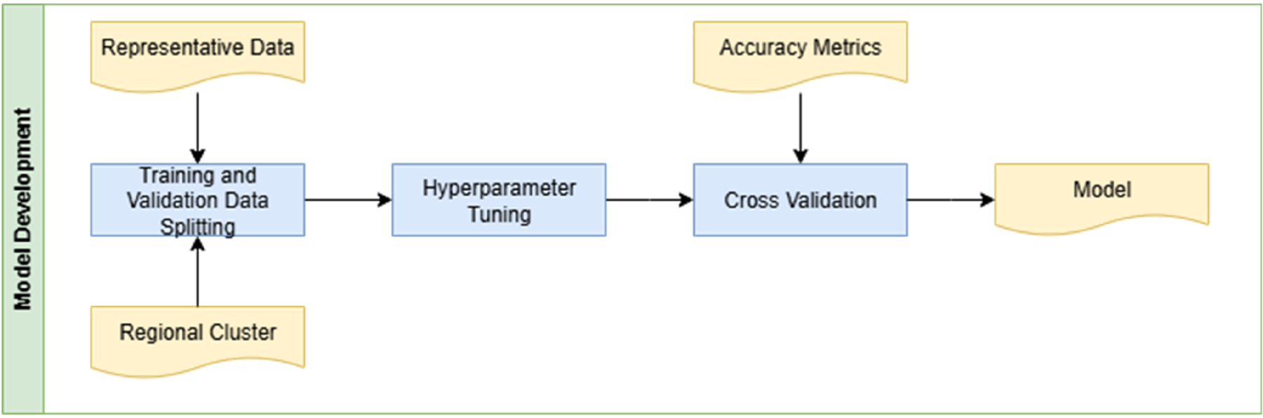
Model development step.
Hyperparameter tuning is conducted using the Optuna library, which efficiently explores parameter ranges to optimize model accuracy. 18 The macro-averaged F1 score is chosen as the optimization objective since it is well-suited for imbalanced classification tasks. 19 A three-fold cross-validation is applied to ensure stability, with tuning centred around critical hyperparameters such as ‘max_depth’, ‘learning_rate’, ‘reg_lambda’, and ‘min_child_weight’. The model uses ‘multi:softprob’ as the objective function for multiclass probability outputs, and early stopping (50 iterations) is implemented to reduce overfitting, supplemented by weighted sampling strategies for handling imbalance (Chen & Guestrin, 2016). Once the optimal parameter set is identified, it is used to finalize the model through a 5-fold cross-validation setup for robust evaluation. To further prevent overfitting, boosting iterations are capped at 10,000 with an early stopping threshold of 1000 rounds. Finally, performance metrics including overall accuracy, F1-Macro, F1-Micro, ROC-AUC, and phase-specific accuracies are averaged across folds to assess generalization.
Using the models developed for each cluster, predictions are generated for all observations from February 2022 to December 2023, with the process depicted in Figure 5. These predictions focus solely on the centroids of each sub-grid, ensuring consistency with ASF observation data, which is also centred on centroids. Additionally, predictions are made at locations corresponding to ASF sample points, effectively simulating the ASF data collection process through machine learning predictions based on ground-truth data. This alignment minimizes discrepancies between predicted and observed data.
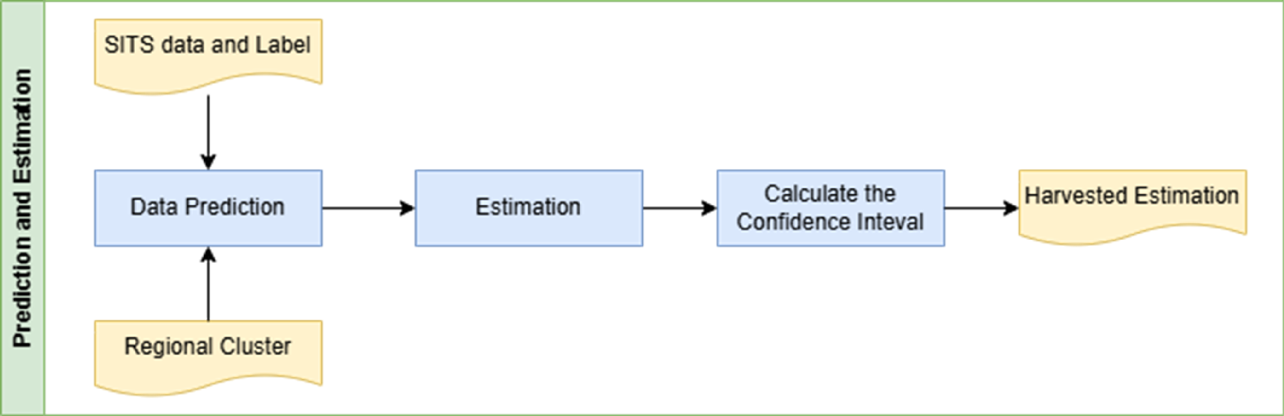
Prediction and estimation step.
The predicted data is then used to estimate paddy phenological stages, following ASF's dot sampling procedure. This approach ensures consistency with ASF's estimation methods. Both point estimates and sampling errors are calculated to evaluate prediction accuracy. The dot sampling method maintains alignment with ASF's approach, while calculating sampling errors provides insights into prediction reliability. Confidence intervals from ASF and this study are compared to assess the level of agreement between the two methods. High alignment suggests that the machine learning model effectively replicates observed data and maintains consistency with field-based measurements, demonstrating the model's reliability and accuracy.
Clustering results
Figure 6 presents the clustering results derived from its agricultural characteristics. Cluster 0, located northwest, is characterized by low elevation, high land surface temperature (LST), low harvested area, and low production, indicating urban and coastal environments. Cluster 1, located on the north, features low elevation and moderate land surface temperature (LST), with intensive paddy cultivation and high productivity, signifying a strong agricultural presence. Cluster 2, located in the northeast, exhibits both urban and agricultural characteristics, with high land surface temperature (LST), and moderate paddy production. Cluster 3, located in the southeast, has moderate elevation but high evapotranspiration, indicative of dense vegetation and less productive agriculture. Cluster 4, located in the south, is characterized by high elevation and low land surface temperature (LST), suggesting fertile highlands yet paddy plantation is not the primary sector. Lastly, Cluster 5, located in the centre, shares similar highland characteristics with abundant vegetation but limited paddy farming.
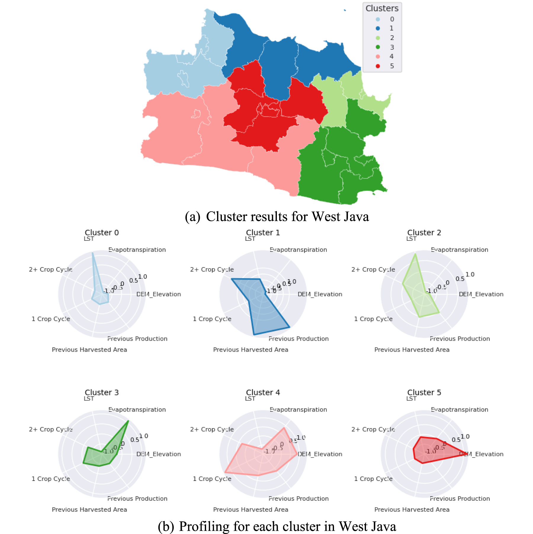
Clustering results in West Java, Indonesia.
Following the cluster results, the data collected undergo the modelling after preprocessing is conducted and Figure 7 represents the data distribution on the training dataset. As depicted in the figure, the presence of imbalanced data can be noted. Cluster 1 consistently exhibits the highest counts across most observation classes excluding the non-paddy and non-vegetation classes. In contrast, Cluster 3 consistently has the lowest counts, primarily for Vegetative 2 and the land preparation classes. The other cluster displays moderate variations for the observation classes, although the highest count of non-paddy and no-vegetation classes is shown in both clusters 0 and 5. The data itself is further modelled with results as presented in Table 2.
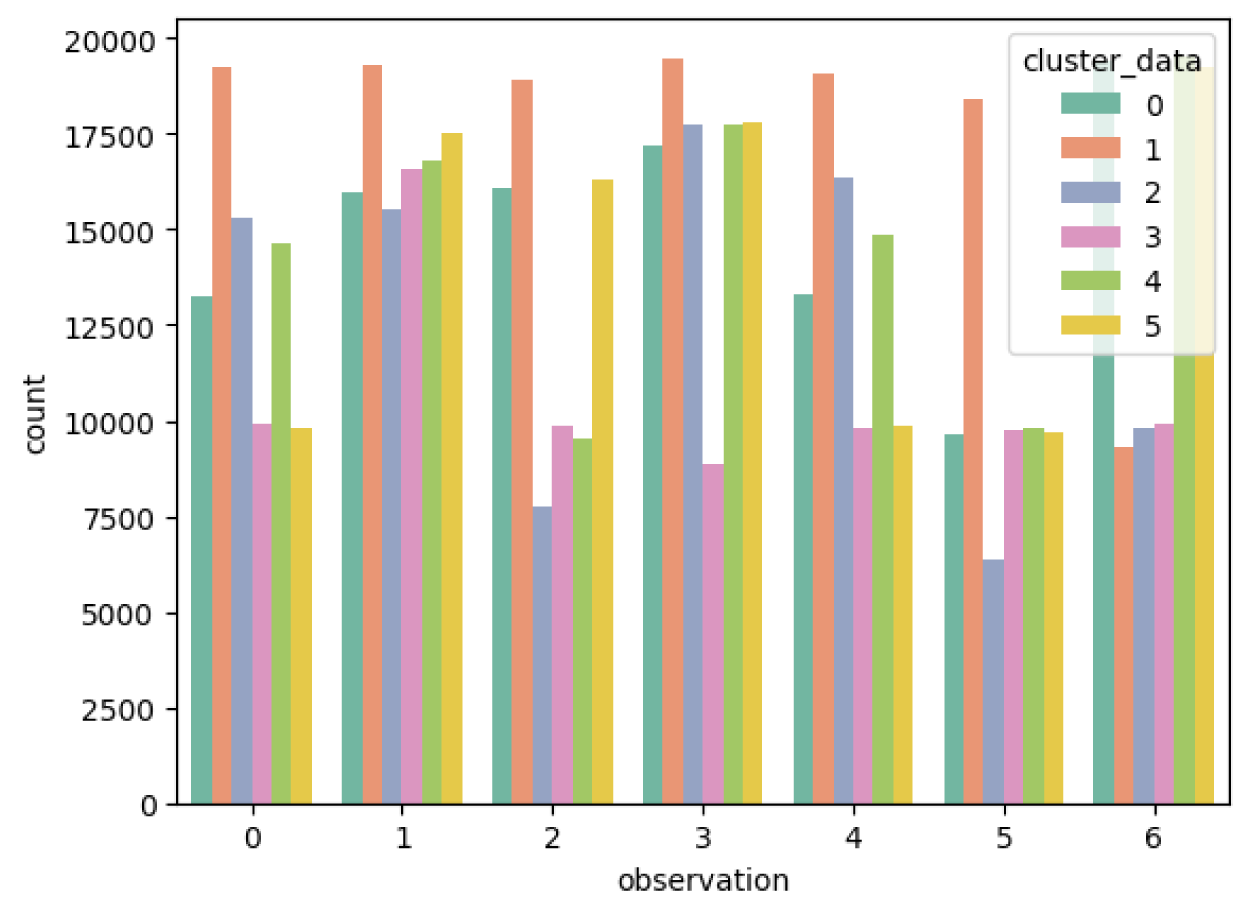
Data distribution on training data.
Accuracy metrics on training and validation dataset.
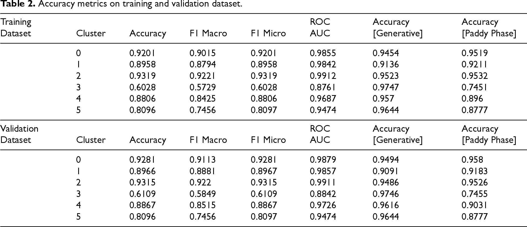
In the training data results, Clusters 0, 1, 2, and 4 achieved accuracy and F1 macro scores exceeding 85%, indicating that the XGBoost model performs optimally in these regions regardless of class imbalance between paddy growth phases. Furthermore, the AUC values for these clusters surpassed 98%, demonstrating the model's strong ability to distinguish between classes. The accuracy for both the generative phase and paddy phase also remained above 85% across these clusters, reflecting the model's consistent performance in identifying paddy growth phases. Conversely, Cluster 3 exhibited significantly lower performance, with an accuracy of 60.28% and an F1 macro score of 57.25%. This suggests that additional attention is required to enhance the model's predictive capability in this region. Cluster 5 also showed suboptimal results, with accuracy and F1 macro scores below 85%, despite achieving a generative phase accuracy of 96.44%. This indicates that while the model struggles overall in this cluster, there is potential for improvement, particularly in the generative phase.
In the validation data results, Clusters 0, 1, 2, and 4 again demonstrated the highest performance, with accuracy and F1 macro scores exceeding 85%. Their AUC values remained above 98%, reaffirming the model's strong classification capability. The accuracy for both the generative phase and the paddy phase was also consistently high, exceeding 90%. However, Cluster 3 continued to show the lowest performance, with an accuracy of 61.09% and an F1 macro score of 58.49%, indicating persistent difficulties in recognizing patterns in this region. Similarly, Cluster 5 maintained accuracy and F1 macro scores below 85%, aligning with the training data results, thus requiring further refinement to enhance model performance, particularly in the paddy phase.
Based on these findings, Clusters 0, 1, 2, and 4 emerge as the most suitable regions for model implementation due to their consistently high performance across all metrics. In contrast, Cluster 5, while underperforming, exhibits potential for improvement, especially in the generative phase, suggesting that further tuning could enhance its predictive capability. These results highlight the necessity of targeted model adjustments to optimize classification accuracy across all clusters, particularly in regions with lower performance.
The model's performance aligns closely with the geographical characteristics of each cluster. Clusters 0, 1, 2, and 4, which are primarily flat or low-elevation regions, demonstrated high accuracy and F1 macro scores exceeding 85%, indicating the model's effectiveness in areas with distinct agricultural, mainly for paddy crops. Their AUC values above 98% further reinforce the model's reliability in distinguishing the paddy phenological stage. In contrast, Clusters 3 and 5, which are characterized by higher elevation, dense vegetation, and complex terrain, exhibited lower performance, with Cluster 3 performing the worst. This suggests that the model struggles in mountainous regions, likely due to environmental variability affecting paddy growth patterns.
Figure 8 depicts the distribution of the paddy phenological stage from February 2022 to December 2023, measured in hectares. Throughout the timeline, fluctuations in each phase are observed. Bareland and Land Preparation exhibit seasonal peaks, notably increasing towards the end of each year. The Vegetative 1 and Vegetative 2 phases follow a similar trend, indicating the progression of paddy growth, with peaks preceding the Generative phase. The Generative phase shows moderate variation, aligning with prior vegetative growth. Harvested areas fluctuate in response to these phases, peaking after the Generative phase. The Non-Paddy and Non-Vegetation categories remain relatively stable.
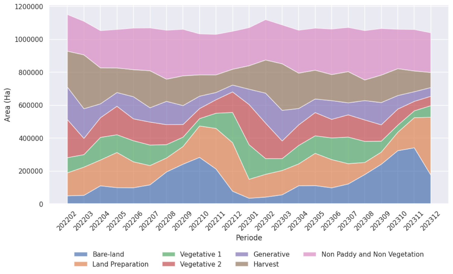
Paddy's phenological stage derived from the prediction.
Figure 9 presents the estimated harvested area derived from the machine learning model and its comparison with ASF data from February 2022 to December 2023. The model reproduces the overall temporal and seasonal patterns observed in the ASF estimates, indicating a strong ability to capture the main dynamics of harvested area. In particular, the primary harvesting peaks in March 2022 and March 2023 are clearly identified, as well as the decline after October 2022 and the inflection point in December 2022 preceding the subsequent increase toward the 2023 peak. The predicted series also reflects secondary peaks in July of both years, which broadly align with fluctuations observed in the ASF data.
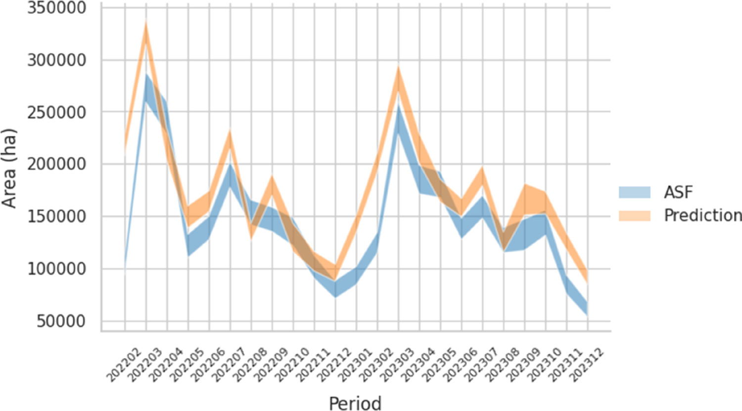
Estimation with confidence interval of harvested area from Feb 2022–Dec 2023.
However, the model exhibits systematic overestimation during several periods, most notably in September 2022, where a pronounced increase is predicted that is not supported by the ASF estimates. As a result, the confidence intervals of the model-based estimates do not overlap with those of the ASF data for substantial portions of the study period. Although overlapping confidence intervals are observed in some months, suggesting partial agreement between the machine-learning estimates and ASF data, this agreement is not consistent over time. Extended periods of overestimation lead to non-overlapping confidence intervals, indicating that the discrepancies between the two approaches are better characterized as moderate rather than minor.
Therefore, the agreement between the machine learning estimates and ASF data should be interpreted primarily in terms of their shared seasonal behavior, rather than as full statistical equivalence. Differences in the width of the confidence intervals further indicate varying levels of uncertainty, with ASF estimates exhibiting greater variability in several months.
Turning to Figure 10, the relative standard error (RSE) analysis provides insight into the precision of both ASF and machine learning–based estimates. The RSE values for both sources remain below 10%, indicating that the estimates meet commonly used quality thresholds for statistical reporting. This threshold is consistent with United Nations guidelines, which recommend relative error margins between 5% and 10% for key indicators intended for analytical and policy applications. 20
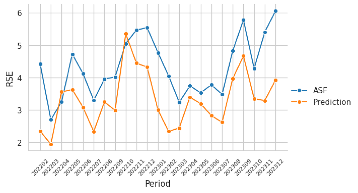
Relative standard error (RSE) of harvested area from feb 2022-Dec 2023.
The machine learning–based predictions generally exhibit lower RSE values than the ASF estimates, indicating a higher degree of internal consistency and temporal stability. However, lower RSE values should not be interpreted as higher accuracy. In several periods, the model produces systematically overestimated values with relatively high certainty, reflecting reduced variability rather than reduced bias. Consequently, while the model delivers stable and precise estimates, these estimates may still deviate from field-based measurements.
Overall, the results highlight the model's strengths in generating stable, low-cost, and temporally consistent estimates that effectively capture seasonal harvesting patterns. At the same time, the presence of systematic bias underscores the need for cautious interpretation when using such outputs for official statistics. Machine learning–based estimates are therefore best viewed as a complementary information source, rather than a direct replacement for field-based data, unless appropriate bias correction or calibration procedures are applied.
In conclusion, this study demonstrates the effectiveness of integrating Satellite Imagery Time Series (SITS) and Area Sampling Frame (ASF) data using machine learning models, specifically XGBoost in West Java, Indonesia. The approach effectively addresses challenges associated with conventional ground-truthing methods, such as high costs and logistical constraints, by leveraging Sentinel-1 radar imagery, which is robust to cloud cover. The results indicate high classification accuracy, particularly in Clusters 0, 1, 2, and 4, where geographic and agricultural characteristics align with model predictions. Conversely, lower performance in Clusters 3 and 5 underscores the need for tailored model adjustments, emphasizing the importance of region-specific characteristics in remote sensing-based agricultural monitoring.
The comparison between ASF data and machine learning–based estimates shows that the proposed approach successfully captures the seasonal harvesting patterns, although systematic overestimation occurs in several periods. The relative standard error (RSE) values of the model-based estimates remain within commonly accepted thresholds, indicating stable and consistent predictions, but lower RSE reflects reduced variability rather than higher accuracy. Overlapping confidence intervals are observed in some months, suggesting partial agreement with ASF data, though this agreement is not consistent over time. Overall, integrating satellite image time series (SITS) with ASF data and machine learning offers a scalable and cost-effective complementary approach for agricultural statistics, particularly for monitoring seasonal dynamics, while highlighting the need for calibration before operational use in official statistics.
Footnotes
Acknowledgements
Sincere gratitude is extended for the “Special Commendation from Developing Countries” during the IAOS Young Statisticians Prize (IAOS-YSP) 2025, granted for this paper. This recognition serves as a valuable encouragement and provides strong motivation for continued research efforts. Deep appreciation is conveyed to the International Association for Official Statistics (IAOS) selection committee for this distinguished honor and their kind support.
Funding
The author received no financial support for the research, authorship, and/or publication of this article.
Declaration of conflicting interests
The author declared no potential conflicts of interest with respect to the research, authorship, and/or publication of this article.