
Abstract
The availability of accurate poverty data at the granular (subdistrict) level remains a significant challenge for official statistics in developing countries, due to limited survey samples, creating information “blind spots” for policy-making. This study aims to address this issue by estimating subdistrict per capita expenditure in Medan Municipality and Langkat Regency by integrating official survey data with geospatial big data. Utilizing a Spatio-Temporal Hierarchical Bayesian Small Area Estimation (ST HB SAE) framework, this research leverages the 2021–2024 National Socioeconomic Survey (Susenas) panel data structure and auxiliary variables from satellite imagery, including Night Time Light (NTL), vegetation index (NDVI), built-up index (NDBI), and air pollutants (NO2). The developed ST HB SAE model incorporates spatial effects (Leroux CAR) and temporal autoregressive (AR1) processes to enhance estimation precision. Results demonstrate that this model significantly outperforms direct estimation and nonspatio-temporal models in terms of Root Mean Squared Error (RMSE) reduction and Coefficient of Variation (CV) stability. Geospatial variables are strongly correlated with welfare indicators, enriching information in sample-deficient areas. Furthermore, a benchmarking process ensures that the estimates are consistent with official regency/municipality level aggregates and meet official statistical standards for operational adoption. This approach offers a cost-effective, robust solution for National Statistical Offices (NSOs) to monitor welfare dynamics in small areas, supporting evidence-based development planning.
Keywords
Background
Poverty remains a primary global concern. 1 SDG-1 affirms the international commitment to end poverty in all its forms by formulating targeted policies based on accurate data. 2 However, National Statistical Offices (NSOs) in many developing countries face a major challenge: the high demand for micro-level data often clashes with limited survey budgets. This measurement challenge in granular domains renders policies ineffective and biased. 3
In Indonesia, although the national poverty rate declined to 9.03 percent in March 2024, 4 regional welfare inequality remains palpable, particularly between urban and rural areas. 5 This inequality reflects structural issues influenced by economic, spatial, social, and environmental factors.6,7 Therefore, poverty measurement that accounts for spatial and temporal variations becomes crucial to observe the dynamics of inequality and policy effectiveness across periods.
Statistics Indonesia (BPS) measures poverty based on average per capita expenditure as a proxy for household economic welfare. Measurement is conducted by comparing per capita expenditure against the poverty line, which reflects the minimum basic needs of households to achieve a decent standard of living. 8 Based on this comparison, households with expenditures falling below the poverty line are categorized as poor.
The National socioeconomic Survey (Susenas) serves as the primary source of poverty data in Indonesia. 9 However, due to sample size limitations, direct estimation from Susenas at the subdistrict level tends to yield high variance and low reliability. Consequently, official poverty data at the subdistrict level remain unpublished, creating an information “blind spot” for local governments that require precise data for allocating social assistance programs. This condition has driven various statistical studies to seek alternative approaches that increase estimation precision without increasing survey burden.
Small Area Estimation (SAE) is a widely used method to produce reliable estimates for more granular areas. This method improves estimation precision by combining information from other variables through a “borrowing strength” mechanism.10,11 Various studies have demonstrated the effectiveness of SAE in reducing poverty estimation variance in small areas without increasing survey costs. 12 Nevertheless, most SAE models currently used assume that each location is independent and static. In reality, welfare phenomena exhibit interregional dependence and intertemporal connections.
SAE studies in Indonesia generally rely on administrative data such as Village Potential (PODES) or census data as auxiliary variables. 13 Although easily accessible, these data are not available annually. PODES data are collected three times within ten years, while census data are updated every ten years. Such conditions render the data unable to reflect current field conditions. The limitations of census and administrative data hamper the model's ability to detect socioeconomic dynamics in the short term. 14 Therefore, alternative auxiliary variables that are more dynamic and can cover small areas continuously are needed.
To fill this methodological gap, this study proposes an approach to modernize official statistics by integrating the Susenas Panel and Geospatial Big Data. Advances in remote sensing technology and geospatial big data processing offer a significant opportunity to enrich SAE models. Geospatial big data indicators have proven to correlate strongly with economic activity and community welfare.15–30 For instance, Night Time Light (NTL) data used in Uganda were able to predict poverty, 26 while Normalized Difference Vegetation Index (NDVI), Normalized Difference Built-up Index (NDBI), and Modified Normalized Difference Water Index (MNDWI) used in Guangzhou were utilized to predict per capita expenditure. 30 Meanwhile, in Indonesia, NTL, NDVI, NDWI, Land Surface Temperature (LST), Carbon Monoxide (CO), Nitrogen Dioxide (NO2), and Point of Interest (POI) data can be used to form multidimensional poverty indices. 16
Such data can be obtained quickly, are relatively inexpensive, and can produce sufficient information to represent the population, 31 making them ideal as auxiliary variables in small area welfare estimation. Furthermore, the use of the Susenas Panel design from 2021 to 2024 offers a unique advantage, as data are collected from the same group of respondents repeatedly. By leveraging this dimension, SAE models can be developed into Spatio-Temporal SAE, where spatial and temporal variations are analyzed simultaneously to produce estimates that are more stable, adaptive, and policy-oriented.
Although the potential for integrating official survey data with geospatial big data has been explored, its application in the Indonesian context remains limited. Most previous studies focused on EBLUP SAE models without accounting for spatial and temporal structures,15,19 composite index creation,16,18 or directly predicting poverty. 17 Few studies have applied the Spatio-Temporal Hierarchical Bayesian SAE (ST HB SAE) framework, whereas this approach allows for more realistic estimation by accommodating inter-regional and inter-period dependence. This limitation indicates a methodological and empirical gap that can be filled by the ST HB SAE approach, especially with the support of Susenas panel data and geospatial big data based auxiliary variables.
This study aims to estimate the average per capita expenditure in every subdistrict in Medan Municipality and Langkat Regency using the ST HB SAE model, which combines the strength of official panel survey data and geospatial big data variables. Methodologically, this study develops the implementation of ST HB SAE based on hierarchical modeling to produce spatially and temporally consistent posterior estimates of average per capita expenditure. Additionally, a benchmarking process is conducted to ensure the consistency of model estimation results with official aggregate figures at the regency/municipality level. This step is crucial so that estimation results can be operationally adopted into the BPS official statistics system. Practically, the research results are expected to support the modernization of BPS official statistics and strengthen evidence-based development planning at the subdistrict level.
Data used
This study integrates official survey data with geospatial big data indicators. The scope of the study covers 44 subdistricts in Medan Municipality (representing urban areas) and Langkat Regency (representing rural areas) over the period of 2021–2024. Medan Municipality and Langkat Regency were selected to represent the distinct urban-rural dichotomy of North Sumatra, as both regions face persistent welfare challenges and slow poverty reduction despite their contrasting economic structures. This integration of survey data with geospatial big data aims to enhance small area estimation while maintaining consistency with the official statistics framework of BPS.
Official survey data ( Susenas panel 2021–2024)
The primary data source utilized in this study is Susenas, conducted by BPS. Unlike conventional cross-sectional approaches, this research leverages the structure of the 2021–2024 Susenas Panel data. The use of panel data enables the model to capture the dynamics of welfare changes within the same households over time, providing crucial temporal information for poverty estimation.
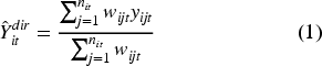
The target variable is the average per capita expenditure (on a logarithmic scale), calculated as total household consumption expenditure on food and nonfood items divided by the number of household members. Direct estimates for each subdistrict are calculated using the following formula:
This study extracts various geospatial big data indicators to serve as auxiliary variables. The selection of variables is grounded in empirical studies demonstrating strong correlations between geospatial big data indicators and economic activity and social welfare.11,15,17,26,30
All datasets were accessed via the Google Earth Engine (GEE) and OpenStreetMap platforms. Each variable was extracted as medium resolution rasters, followed by pre-processing steps including cloud masking, median compositing, and radiometric normalization to ensure quality and interannual consistency (Table 1). To maintain temporal alignment with the observations, all imagery was compiled during the March–July period of each year, coinciding with the Susenas data collection schedule. Subsequently, each raster layer was aggregated to the subdistrict level by calculating the mean value within administrative boundaries using official BPS shapefiles and the WGS-84 (EPSG 4326) projection system. The processing yielded a spatio-temporal panel dataset comprising six geospatial variables (Table 1) across 44 subdistricts (21 in Medan Municipality and 23 in Langkat Regency) over four observation years (2021–2024).
Description of geospatial big data sources, variables, and preprocessing specifications.
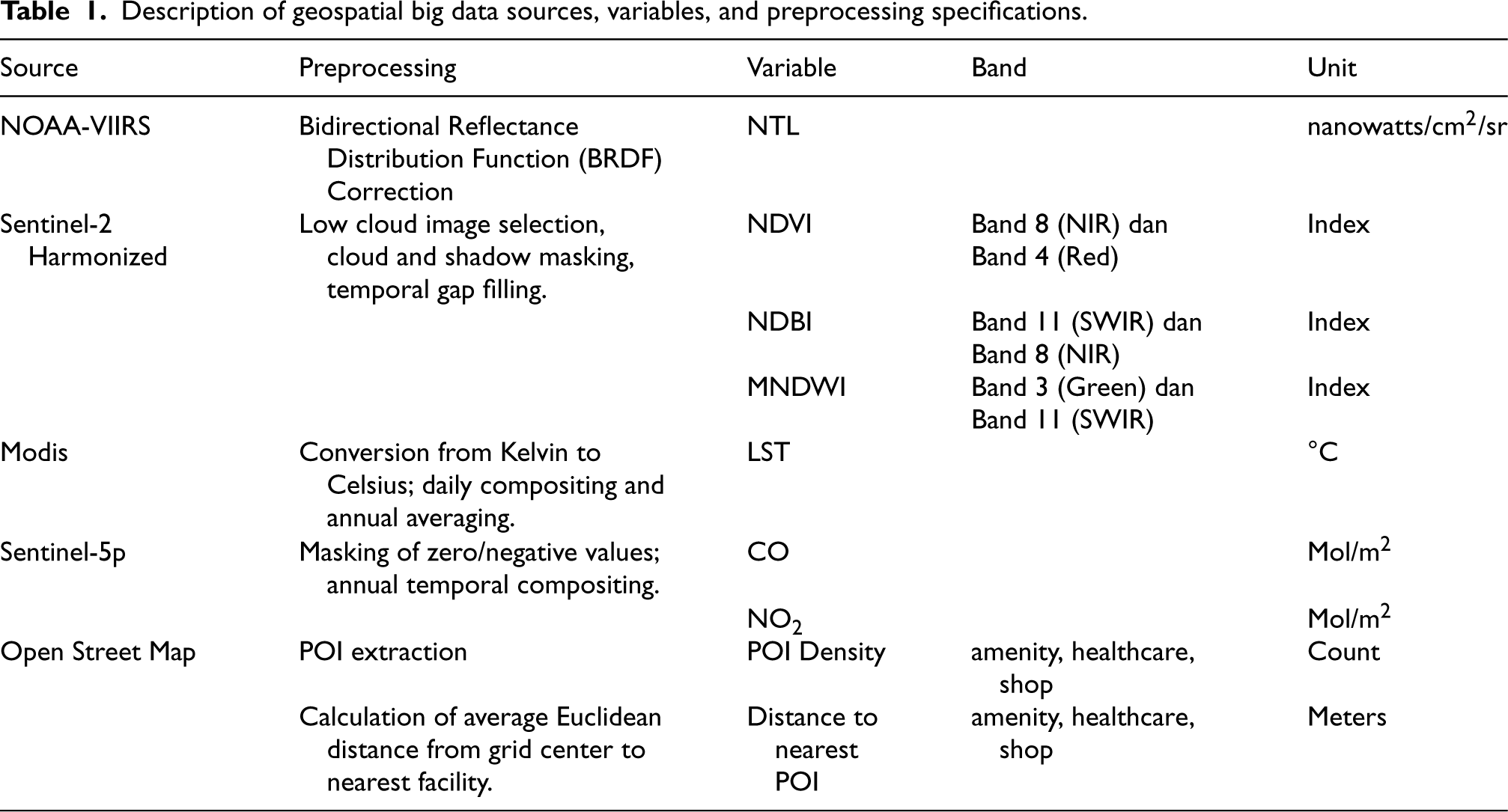
Description of geospatial big data sources, variables, and preprocessing specifications.
The research methodology is designed through five systematic stages: (1) selection of auxiliary variables, (2) variance smoothing, (3) Spatio-Temporal Hierarchical Bayesian modeling, (4) parameter estimation and inference, and (5) evaluation and benchmarking.
Selection of auxiliary variables
The initial step is to select geospatial big data variables that exhibit a strong linear relationship with per capita expenditure. The selection was conducted using Pearson correlation (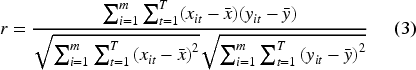
Where r denotes the Pearson correlation coefficient,
Direct estimates from Susenas at the subdistrict level often exhibit unstable variances due to small sample sizes. To address this issue, the Generalized Variance Function (GVF) approach is employed, with the form
36
:
Where 
Thus, the smoothing model is written in equation (5) as follows:
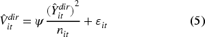
With
This study extends the Fay-Herriot (FH) model into a Spatio-Temporal Hierarchical Bayesian framework by incorporating the likelihood, the linking model, and spatial and temporal random effects. The likelihood is defined as in equation (6):

Where 
Where 
The proper CAR distribution is defined with respect to the adjacency matrix 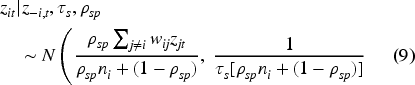
Where 
Where
The priors for the regression coefficients are presented in equation (11), where the coefficients are assumed to follow a normal distribution with mean 0 and standard deviation 5. Gelman
38
emphasize that a Normal (0, 5) prior is sufficiently broad to accommodate potential variations in effects, yet remains narrow enough to maintain Markov Chain Monte Carlo (MCMC) convergence stability and avoid the common issues associated with overly flat non-informative priors.

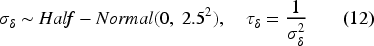
The year effect is defined by setting 
The primary posterior quantity of interest is 
Parameter estimation was performed using the MCMC simulation approach with the Gibbs Sampling algorithm using R-Studio with the tipsae 36 and nimble. 39 The simulation was run for 10,000 iterations, with the first 5000 discarded as a burn-in period to ensure chain stability, and every 5th iteration retained (thinning = 5) to reduce autocorrelation between samples.
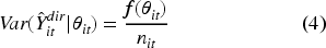
Model performance was evaluated using four primary indicators: the Coefficient of Variation (CV), Root Mean Squared Error (RMSE), Coverage Probability (CP), and a goodness of fit test based on the Wald statistic. Since the true population parameters are unobserved, model evaluation relies on the design-based direct estimates as a reference benchmark. Following Rao and Molina, 11 the CV, RMSE, and CP are calculated by treating the direct estimates as proxies for the true values.
The precision of the estimation results using the CV is calculated using the following formula:
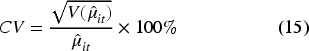
Where 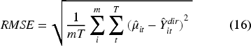
Where 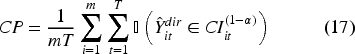
Where 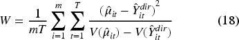
Where
To strengthen the inferential assessment of model performance, we complement the descriptive metrics with a distribution-free comparison of predictive accuracy. Specifically, we apply a two sample Kolmogorov-Smirnov test to compare the distribution of absolute prediction errors between the best model and alternative models, without relying on parametric assumptions. 42
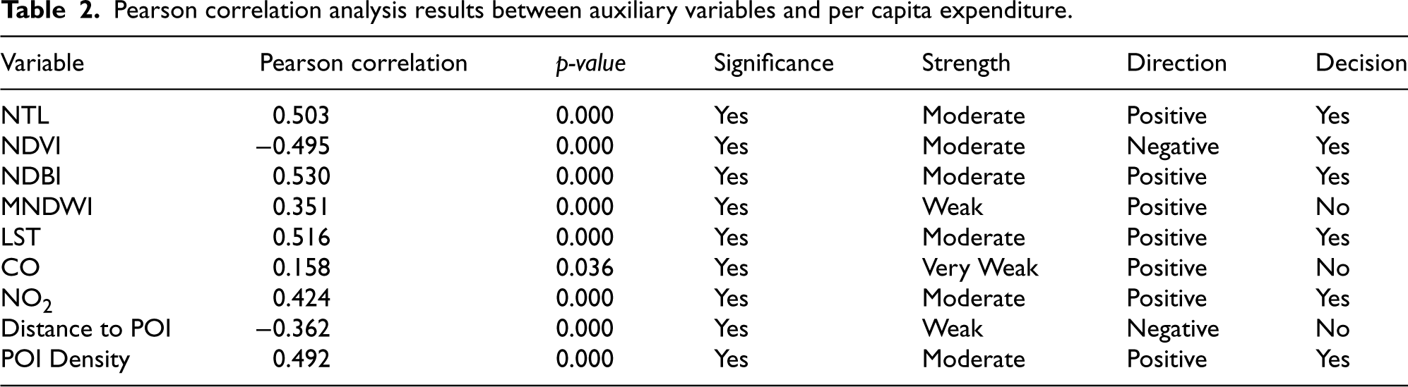
Pearson correlation analysis results between auxiliary variables and per capita expenditure.
Benchmarking was conducted using the raking method (iterative proportional fitting). This process is performed to meet official statistical standards, requiring that the final SAE estimates be consistent with aggregate figures published by BPS. The equation is as follows:
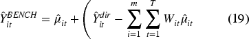
Where 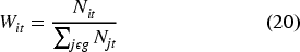
The auxiliary variables used in the model are those exhibiting moderate to strong correlations (|r|>0.4) as correlation coefficients above 0.4 indicate a moderate relationship deemed sufficiently relevant for further analysis. 35 Table 2 shows that six variables NTL, NDVI, NDBI, LST, NO2, and POI Density were selected as auxiliary variables. Furthermore, variance smoothing was conducted. As illustrated in Figure 1, the difference is evident that prior to smoothing, the variance dispersion was extremely wide with extreme values; however, after smoothing, the variances were corrected to become more stable with a narrower dispersion. 43
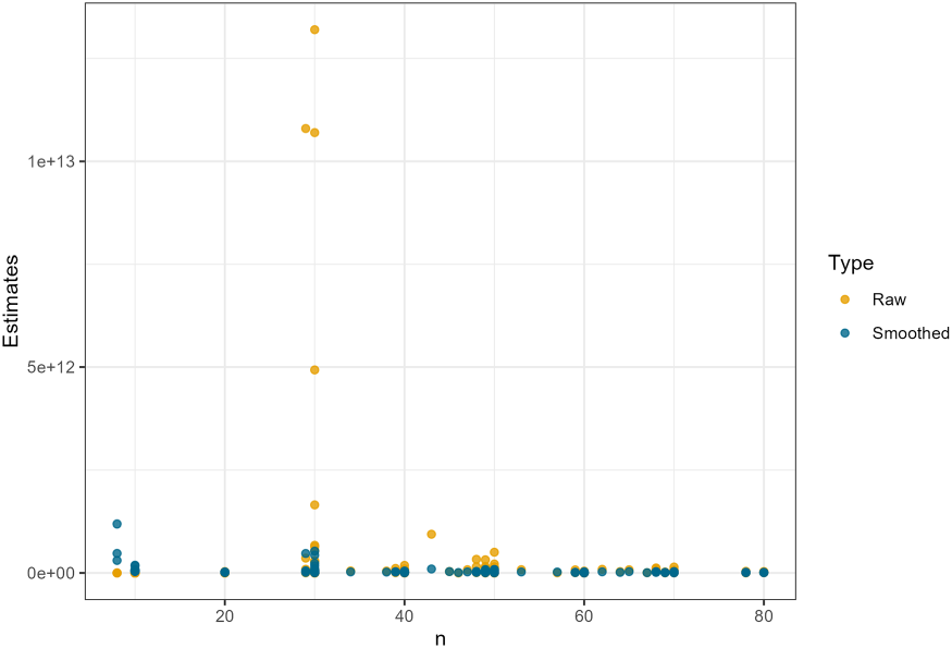
This study compares four models: the HB model without spatio-temporal effects, the HB model with spatial effects, the HB model with temporal effects, and the HB model with spatio-temporal effects. The posterior mean results are presented in Table 3. Furthermore, Table 3 reveals that the relationship between the average posterior fixed-effect values and the average per capita expenditure varies across models. Notably, the model with spatio-temporal effects exhibits a pattern consistent with the prior correlation analysis. However, this observation alone does not demonstrate that the spatio-temporal model is superior to the others. Therefore, several diagnostic tests are necessary to assess model reliability and select the best model for benchmarking.
Comparison of variance before smoothing (raw) and after smoothing (smoothed).
Posterior fixed effect estimation results of SAE model.
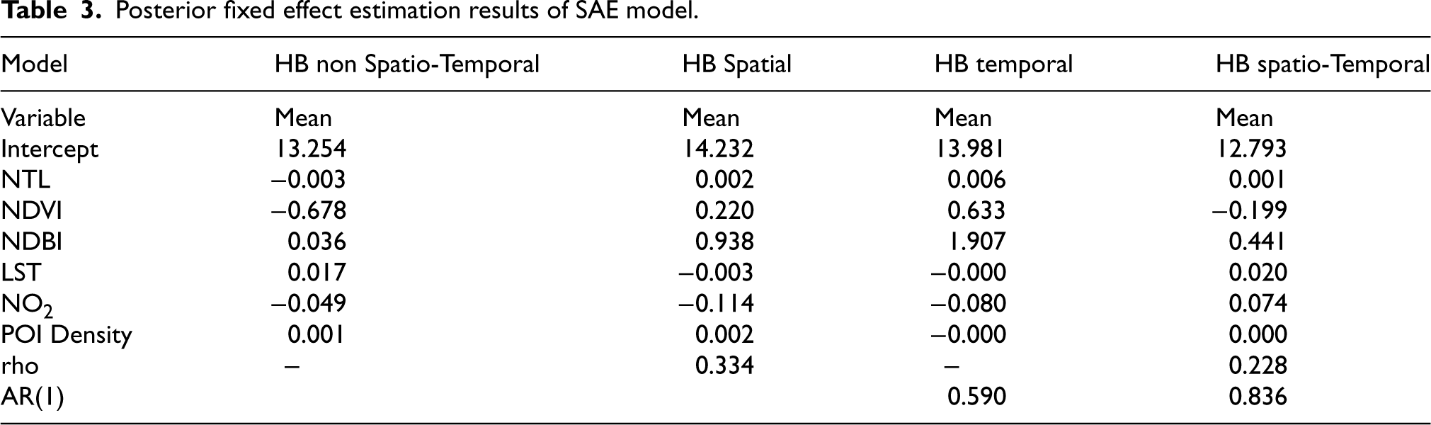
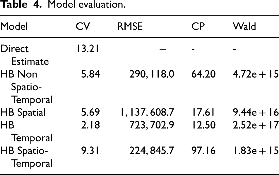
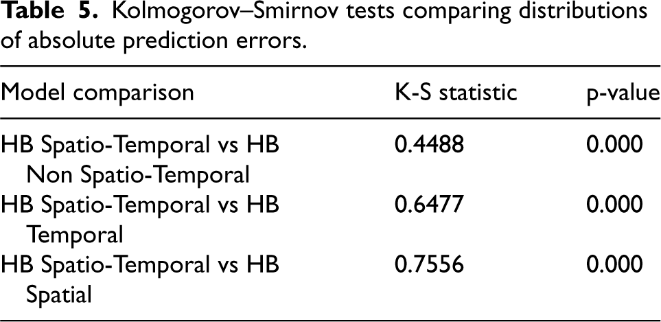
First, a check for model consistency is required, as the HB method employed applies computational sampling via MCMC. Figure 2 shows that each model is relatively consistent, with residuals tending to decrease as the sample size increases. In comparing models, the spatio-temporal model performs best, with residuals most tightly clustered around zero for both small and large samples. Next, Table 4 presents several indicators to assess and compare model performance which is complemented by an examination of the violin plot of the CV distribution in Figure 3. Furthermore, the results of the Kolmogorov–Smirnov tests (Table 5) provide inferential support for the observed performance differences. The p-values for all model comparisons are significantly lower than 0.05, indicating that the reduction in estimation error is statistically significant and consistent across the entire distribution. Taking all these indicators into account, it can be concluded that the HB Spatio-Temporal model is the strongest candidate. Overall, the proposed spatio-temporal framework demonstrates improved precision, reduced estimation bias, and a more coherent characterisation of uncertainty, supporting its suitability for small-domain estimation within official statistics.
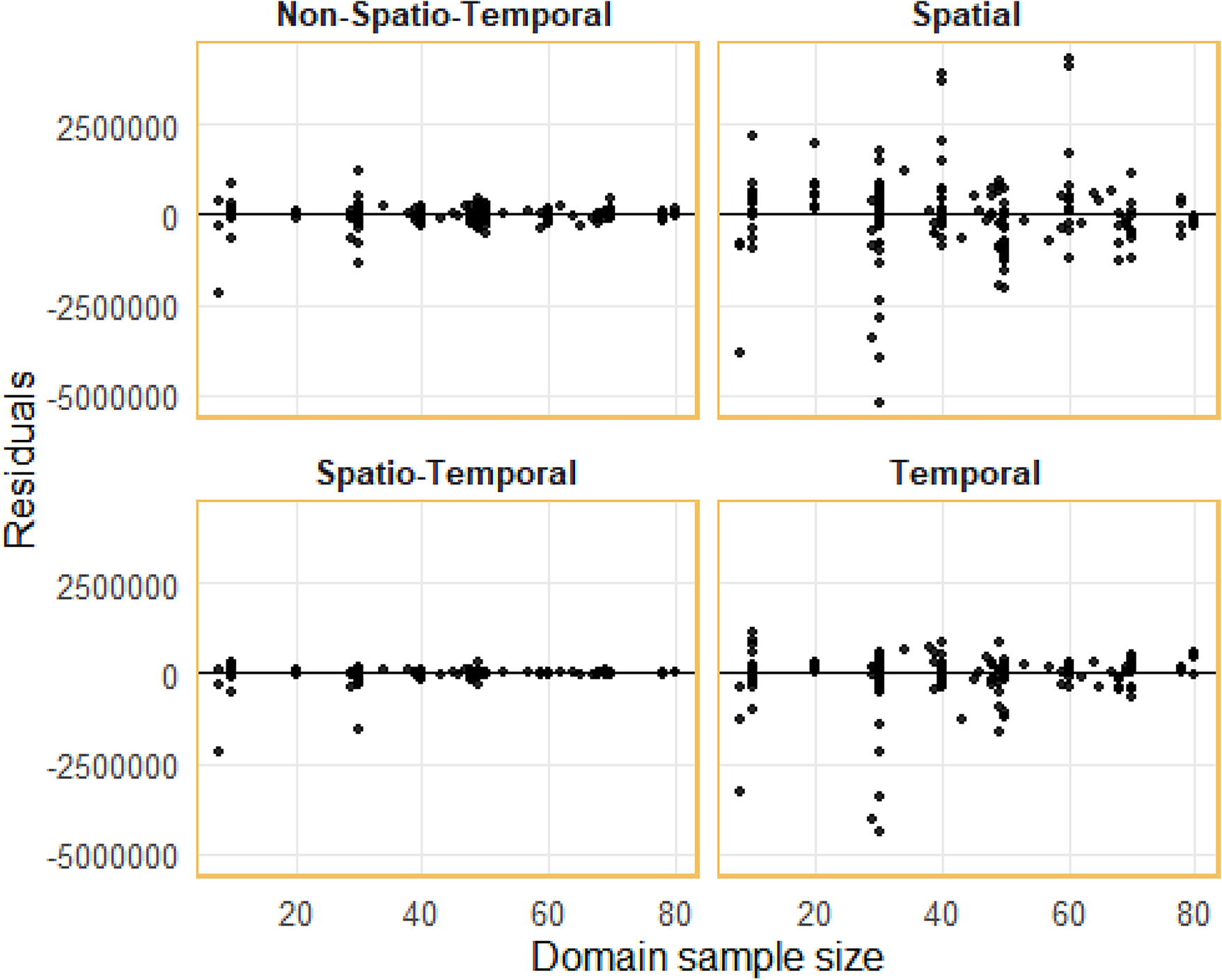
Scatterplot of residual model and number of samples.
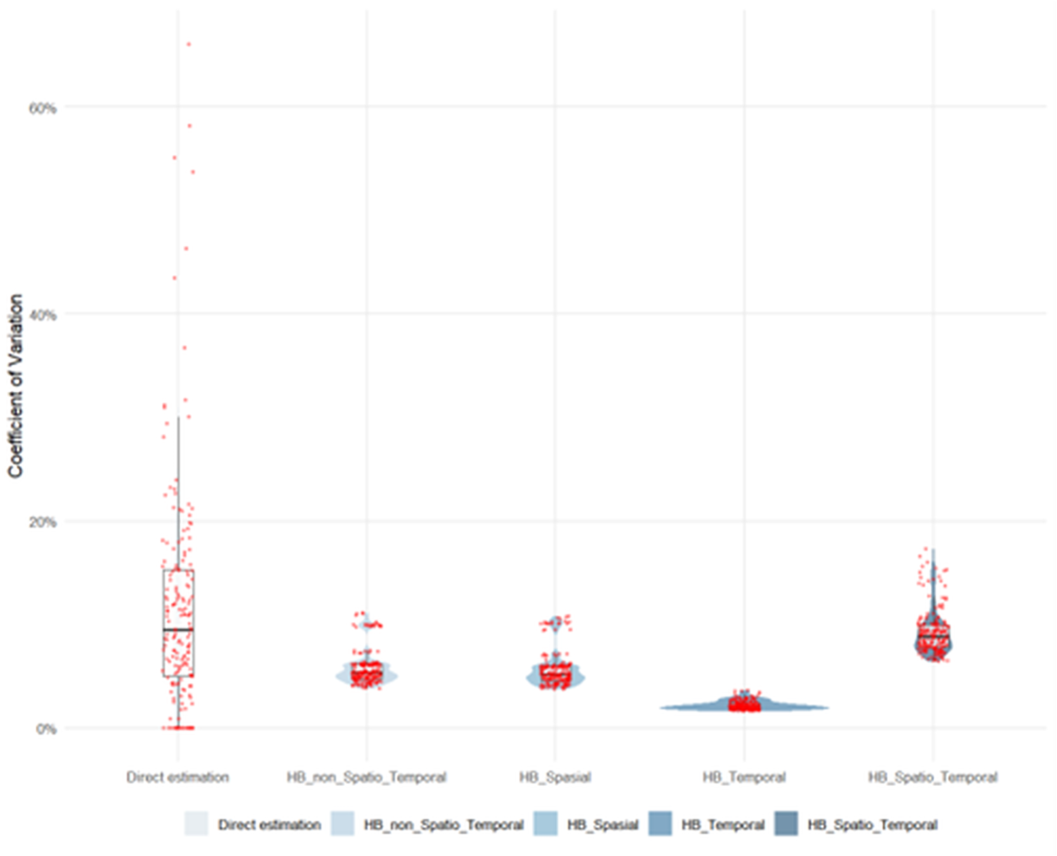
CV distribution using violinplot, boxplot and scatterplot.
Model evaluation.
Kolmogorov–Smirnov tests comparing distributions of absolute prediction errors.
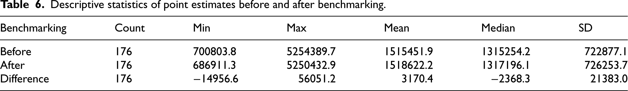
The HB Spatio-Temporal model was selected for further analysis. Consequently, benchmarking was conducted to ensure that the subdistrict level estimation results are consistent with the official aggregate results at the regency/municipality level. Table 6 presents the point estimates of the subdistrict average per capita expenditure before and after the benchmarking process. In general, it can be observed that the point estimates before and after benchmarking do not differ significantly. Specifically, the boxplot (left) shows that the distribution of per capita expenditure estimates across subdistricts remains relatively unchanged after benchmarking (Figure 4). The median values, quartile dispersion, and the presence of outliers are nearly identical between the pre and post benchmarking conditions. Furthermore, the scatterplot (right) also indicates a near perfect fit (R2 = 1) between the two estimates.
Descriptive statistics of point estimates before and after benchmarking.
The consistency of the estimation results is further assessed through spatial visualisation. Figure 5 presents the spatial distribution of per capita expenditure across 44 subdistricts in Medan Municipality and Langkat Regency for the year 2024. The side-by-side comparison indicates that the spatial patterns remain highly consistent before and after the benchmarking process. Areas with higher expenditure levels continue to be concentrated in Medan, while predominantly subdistricts in Langkat remain associated with lower expenditure levels. These findings suggest that the benchmarking procedure introduces only limited local adjustments while preserving the underlying spatial relationships captured by the spatio-temporal hierarchical Bayesian small area estimation model.
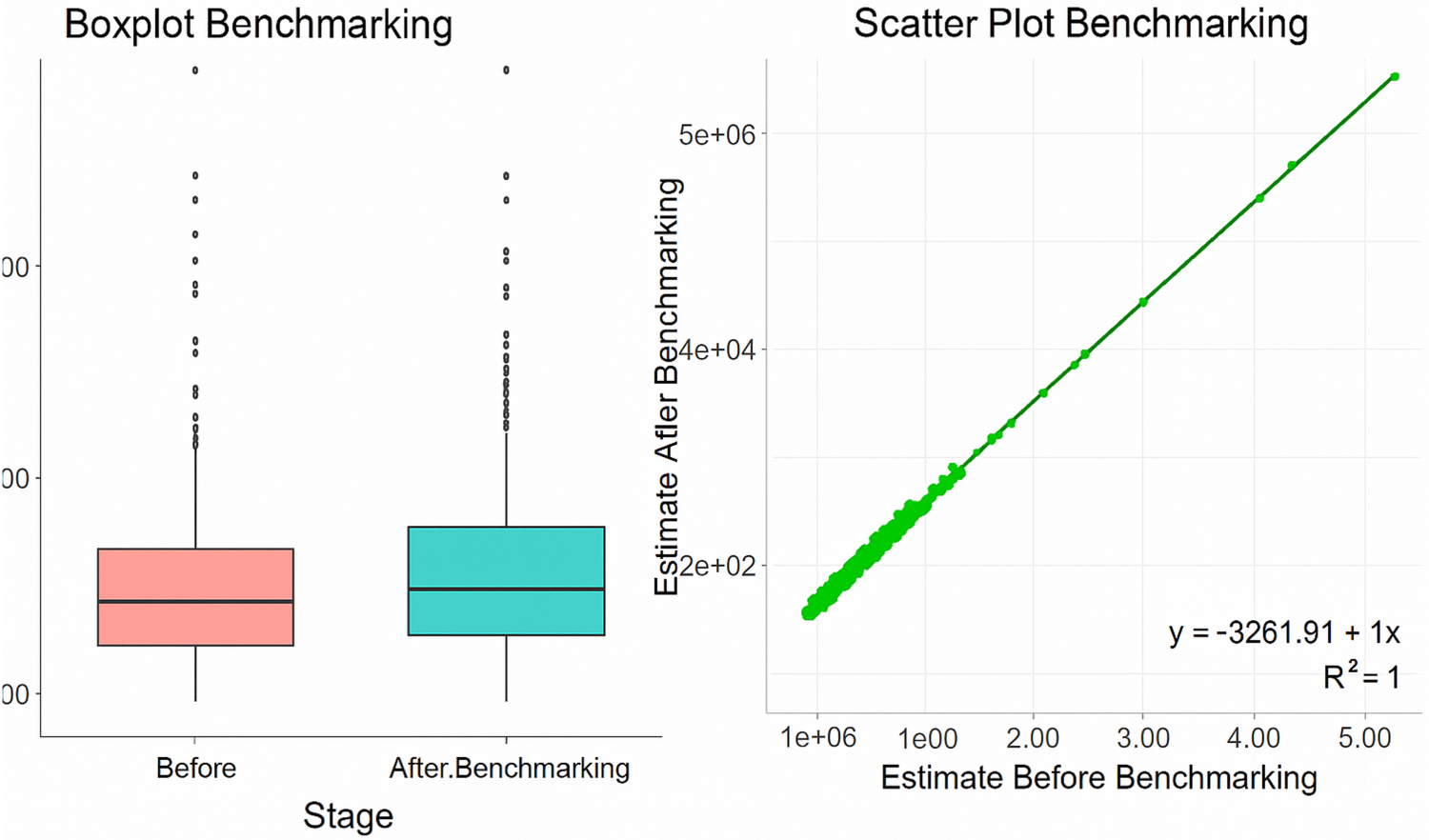
Comparison of estimates before and after benchmarking.
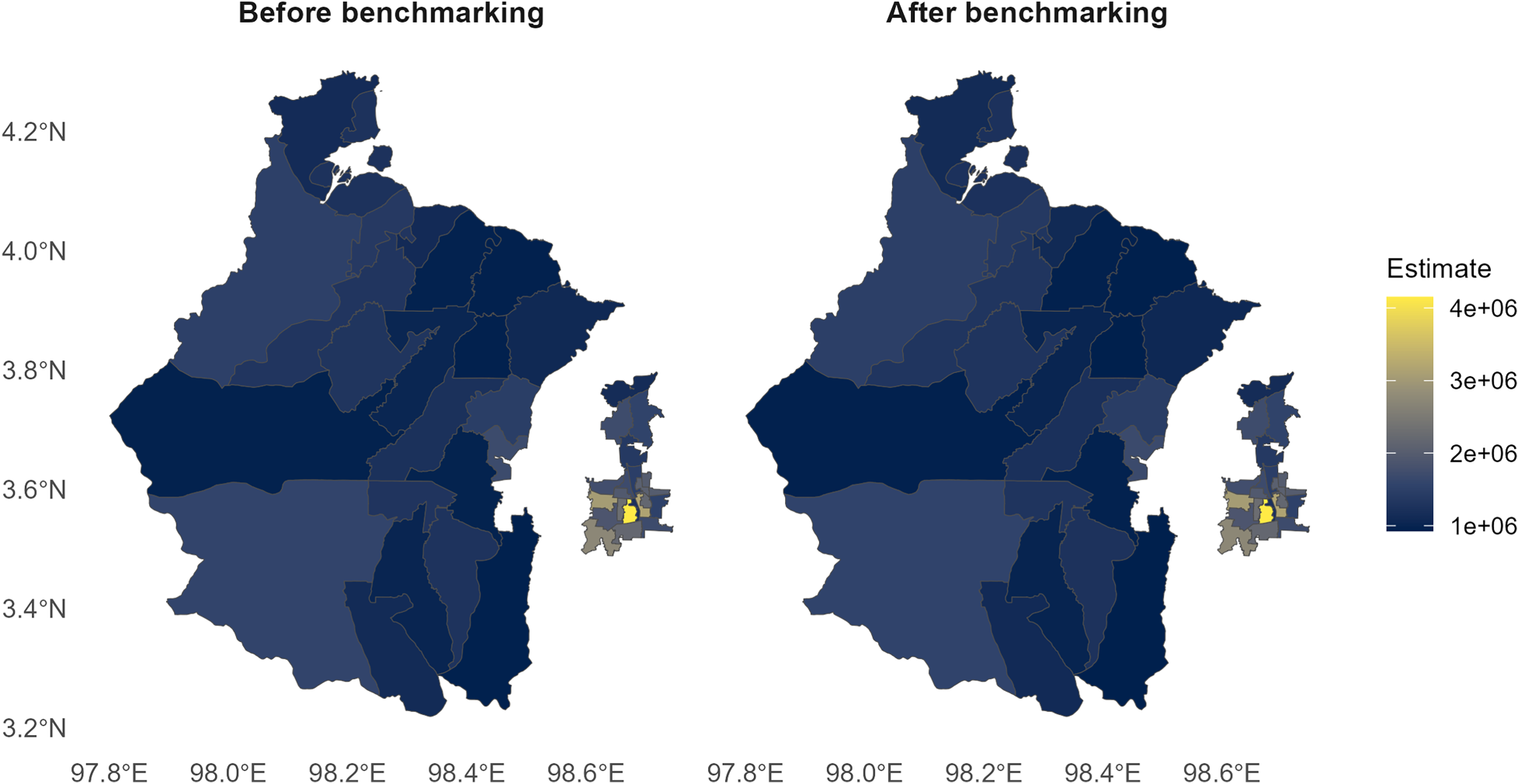
Comparison of spatial distribution of subdistrict per capita expenditure in Medan and Langkat (2024): before benchmarking (left) and after benchmarking (right).
This study demonstrates that applying Spatio-Temporal Hierarchical Bayesian Small Area Estimation (ST HB SAE) effectively improves the accuracy of average per capita expenditure estimates at the subdistrict level. Compared to direct estimation from Susenas, the spatio-temporal model provides significantly more precise and stable results, particularly in subdistricts with small sample sizes. These findings confirm that modeling based on “borrowing strength” through spatial (CAR) and temporal (AR1) components can overcome the primary limitations of official surveys in small domains.
The integration of geospatial big data has also proven to provide a significant contribution to strengthening the SAE model. Variables such as NTL, NDBI, NDVI, LST, and NO2 exhibit consistent correlations with household expenditure, thereby enriching the model's information. These indicators capture variations in physical, environmental, and economic activity not covered in official survey data or conventional administrative records. This result aligns with recent studies emphasizing the potential of remote sensing indicators for measuring socioeconomic dynamics and demonstrates that integrating geospatial big data offers tangible added value in the Indonesian context, which features contrasting urban rural characteristics.
In the context of model implementation, ST HB SAE exhibits superior performance compared to nonspatial models and spatial models without a temporal component. The improvement in precision is reflected in the significant reductions in CV and RMSE, as well as in the high coverage probability. Furthermore, the consistency of results against official aggregates following the benchmarking process (adjustment < 1 percent) indicates that this model aligns with official statistical standards and can be integrated into existing statistical production frameworks.
From a regional substantive perspective, spatial patterns reveal a higher concentration of per capita expenditure in Medan's urban centers, whereas agrarian areas in Langkat consistently remain in the lower quantiles. Temporal trends from 2021 to 2024 show a stable increase in household expenditure, indicating the post-pandemic economic recovery. The spatio-temporal model successfully captures these patterns more smoothly and realistically compared to direct estimation, which tends to be fluctuating.
Overall, the findings of this study support the initial research objectives that the ST HB SAE model produces average per capita expenditure estimates that are more precise, temporally stable, and sensitive to spatial differences. From a policy perspective, this approach offers a stronger foundation for local governments and BPS to monitor welfare dynamics at the subdistrict level, strengthen the basis for targeting social programs, and drive the modernization of official statistics through the utilization of geospatial big data and Bayesian methodologies. Nevertheless, this study also offers opportunities for further development, such as integrating higher spatial resolution, using dynamic administrative data, or expanding the model to other regions to assess the method's generalizability.
Conclusions
This study demonstrates that applying ST HB SAE effectively improves the accuracy of average per capita expenditure estimates at the subdistrict level in Medan Municipality and Langkat Regency. Compared to Susenas direct estimates, the spatio-temporal model produces estimates that are more precise, temporally stable, and capable of covering non-sampled subdistricts. The geospatial auxiliary variables used in this study NTL, NDVI, NDBI, LST, NO2, and POI indicators show statistically significant relationships with household expenditure, as indicated by correlation tests. Although the correlation strengths vary across variables, all indicators contribute positively to the model's predictive capability. These results underscore the potential of geospatial data as a relevant source of supplementary information for small area estimation, particularly in regions lacking annually updated administrative data.
The application of ST HB SAE also yields superior performance compared to nonspatial models and spatial models without a temporal component, as reflected in reduced CV and RMSE and increased coverage probability. The consistency with official aggregates following benchmarking demonstrates that this model meets the requirements of official statistics and can serve as a complement to welfare estimation at the subdistrict level.
Overall, these findings support the use of the Susenas panel, combined with geospatial big data, to produce more accurate small area estimates. This model has the potential to assist local governments in identifying regional inequalities more precisely and strengthening evidence based development planning. Going forward, future research could explore integrating higher resolution geospatial data, incorporating dynamic administrative variables, or applying the model to other regions to test the generalizability of this approach.
Footnotes
Acknowledgments
This manuscript is a portion of the first author's doctoral research. The authors wish to express their gratitude to The Graduate School, Universitas Gadjah Mada, for granting access to literature and research resources, to BPS for providing the data, and to the Indonesia Endowment Fund for Education or Lembaga Pengelola Dana Pendidikan (LPDP) under the Ministry of Finance of the Republic of Indonesia for sponsoring the author's doctoral degree.
Funding
The authors received no financial support for the research, authorship, and/or publication of this article.
Declaration of conflicting interests
The authors declared no potential conflicts of interest with respect to the research, authorship, and/or publication of this article.