
Abstract
Radial Basis Function Neural Networks (RBFNNs) are frequently used in UAV disturbance estimation. However, the number of center points and the width values of the activation function significantly affect estimation accuracy, and selecting appropriate values empirically is challenging. Therefore, evolutionary optimization algorithms such as Particle Swarm Optimization (PSO) are often employed to determine the optimal parameters. Nevertheless, these evolutionary algorithms may suffer from premature convergence or entrapment in local optima, causing the fitness function value to stagnate. To address this issue, this study proposes a K-Means initialization-based two-stage particle swarm optimization algorithm (KTS-PSO-RBFNN) for RBFNN parameter optimization. The proposed method initializes the basis function centers and widths via K-Means clustering and optimizes them in two stages: first, jointly optimizing the centers and widths to locate the global optimal region; then, fine-tuning the widths while fixing the centers to eliminate parameter coupling interference. To comprehensively evaluate the proposed method, synthetic data comparative experiments, Dryden wind disturbance experiments, cross-validation experiments, and real-world dataset experiments were conducted. The results demonstrate that the KTS-PSO-RBFNN consistently outperforms traditional baseline algorithms across all test scenarios. The proposed method achieves lower fitness function values, demonstrating superior prediction accuracy in UAV disturbance estimation.
Keywords
Introduction
Unmanned Aerial Vehicles (UAVs) have become increasingly integral to contemporary military, civil, and commercial operations, with applications including reconnaissance, disaster surveillance, precision agriculture, and logistics delivery. Notably, UAVs have been widely adopted in agricultural plant protection (covering over 80% of farmland in China) and logistics delivery (e.g., 94 new UAV logistics routes in Shenzhen with 776,000 annual cargo flights in 2024). However, when UAVs fly in complex environments, they suffer from various external disturbances, such as gust interference, airflow turbulence, and changes in mass characteristics caused by load variations (Geronel et al., 2023; Ijaz et al., 2024; Park et al., 2023). These disturbances not only seriously affect the flight quality and control accuracy of UAVs but also may endanger mission reliability and even lead to flight accidents. Therefore, developing effective methods to accurately estimate and compensate for unknown disturbances, while enhancing the robustness and adaptability of UAVs in uncertain environments has become a major challenge in UAV research (Chen et al., 2022; Hou et al., 2023; Zuo et al., 2022).
Most traditional disturbance estimation approaches rely on accurate mathematical models, including disturbance observers, Kalman filtersand their variants. Although these methods perform well under ideal conditions, their performance relies heavily on accurate UAV dynamic models. In practical applications, it is often difficult to obtain a precise mathematical model, and the model fails to account for all unknown disturbances and uncertain factors. The terrain-following estimation methods proposed in Kadri and Yousuf (2025); Taame et al. (2023) improved the position estimation accuracy by fusing multi-sensor data through Kalman filters, but they are still ineffective when facing complex airflow disturbances. As Artificial Intelligence (AI) technology matures, intelligent control systems are unlocking innovative approaches to tackling this long-standing issue. The Generative Artificial Intelligence (GenAI) (Wang et al., 2025a) is introduced as a novel interference suppression method, designed for state information estimation and adaptive disturbances suppression, thereby achieving consistency with the interference estimation. An intelligent control algorithm based on Adaptive Dynamic Programming (ADP) was proposed in Hu et al. (2022), introducing a cost function based on zero-sum games to eliminate model uncertainties, which is used to solve the attitude tracking problem of re-entry vehicles affected by both model and state uncertainties. ADP-based optimal control for discrete-time systems with safe constraints and disturbances was studied in Ye et al. (2025). Studies in Xia et al. (2020); Zhang et al. (2023); Wang et al. (2022) showed that the integral sliding mode controller based on ADP, combined with a Radial Basis Function Neural Network (RBFNN) observer, can effectively solve the problem of time-varying input disturbances in UAV trajectory or attitude tracking.
As a feed-forward neural network, RBFNN has the advantages of simple structure, fast convergence speed, and the ability to approximate any nonlinear function, making it a powerful tool for system identification and disturbance estimation (Hosseini et al., 2023; Jiang et al., 2022; Liu et al., 2023). RBFNN uses nonlinear radial basis functions as the activation functions of the hidden layer and combines them with a linear output layer, which can approximate any continuous function with arbitrary (Hartman et al., 1990; Park & Sandberg, 1991). This makes it very suitable for handling nonlinear disturbance estimation problems in UAV systems. Studies in Ouyang et al. (2021); Guo et al. (2022); Wei et al. (2024); Xiong and Chen (2025) demonstrated the advantages of RBFNN in UAV control for unknown parameter estimation and uncertain disturbance estimation.
Despite these advancements, RBFNN still faces challenges such as dependence on network parameter selection, including the centers and widths of basis functions. These parameters are usually trained via gradient descent, which often converges to suboptimal solutions and is sensitive to initial values, thereby compromising the final estimation accuracy and generalization ability (Jiang et al., 2022). A novel Large Language Model-guided method was proposed in Li et al. (2025) to adaptively adjust hyperparameters and eliminate redundant exploration. These studies provide the motivation to explore a method for the rapid optimization of RBFNN parameters.
The Particle Swarm Optimization (PSO) algorithm is a swarm intelligence-based optimization algorithm inspired by the social behavior of bird flocks or fish schools, proposed by Kennedy and Eberhart in 1995 (Kennedy & Eberhart, 1995) and further studied by Kennedy in 1997 (Kennedy, 1997). The PSO algorithm finds the optimal solution through collaboration and information sharing among individuals in the swarm. Each particle represents a candidate solution in the solution space and updates its position and velocity by tracking the individual extremum (pbest) and the global extremum (gbest). Compared with other heuristic methods, the PSO algorithm effectively improves the global search and local optimization capabilities by flexibly balancing the mechanisms of individuals and the swarm (Oh et al., 2012).
In UAV-related research, the PSO algorithm has demonstrated excellent performance. By combining PSO with an adaptive neuro-fuzzy inference system (ANFIS), the study in Selma et al. (2020) improved the trajectory tracking performance of UAV compared to the ANFIS and Proportional-Integral-Derivative (PID) methods. The study in Konar and Chatterjee (2025) reported the design of an extended fuzzy state observer based on PSO and the research on disturbance rejection in quadrotor sliding mode attitude control. This study reconstructed the extended state observer using Takagi-Sugeno (TS) fuzzy logic and combined it with PSO based automatic parameter tuning to form a dual-channel disturbance rejection architecture, which significantly improved the tracking performance and noise suppression capability of the observer. Recent studies (Can, 2026; Can, 2025) further validate the advantages achieved by combining PSO and fuzzy logic in UAV control methods. These achievements have proved the effectiveness of the PSO algorithm in solving complex UAV control problems.
However, PSO algorithm is sensitive to the parameters selection (such as learning factors and inertia weight) and may converge prematurely to sub-optimal solutions, especially when dealing with complex and multi-modal problems. Particles will gather near suboptimal solutions, which hinders the exploration of other potential regions in the search space (Sonny et al., 2023). The authors of Li et al. (2014) solved this premature convergence problem by introducing diversity maintenance techniques, such as adding random disturbances to particle positions. Another drawback of the PSO algorithm is that it may fall into suboptimal solutions, especially in complex problems with multiple suboptimal solutions and one global optimal solution. A study by Rini et al. (2011) increased the chance of escaping from suboptimal solutions and finding better solutions using swarm diversity indicators and restart strategies. Researchers in Chai et al. (2021) designed an evolutionary restart strategy to enhance its ability to avoid falling into local infeasible regions.
To address the challenges of RBFNN's high dependence on network parameter selection and parameter optimization, the PSO algorithm is implemented into RBFNN. The global search capability of PSO is used to automatically optimize and determine the key parameters of RBFNN. This fusion method takes the advantages of both algorithms: the PSO algorithm is responsible for the global optimization of RBFNN parameters to avoid converging to suboptimal regions; while the optimized RBFNN is responsible for accurate estimation of the complex disturbances suffered by UAVs, thereby constructing a high-performance UAV disturbance estimator. This PSO-RBFNN hybrid framework solves the problem of RBFNN parameter sensitivity through an intelligent optimization algorithm. On the other hand, it provides a disturbance estimation method that does not rely on accurate mathematical models and has inherent robustness to model uncertainties and unmodeled dynamics. The study in Tang et al. (2023) confirmed the effectiveness of the improved PSO-RBFNN adaptive sliding mode controller where the adjustment time of the quadrotor system has improved by approximately 50–75%, showing excellent trajectory tracking speed and anti-interference ability. In terms of neural network optimization, researchers (Wang et al., 2025b) optimized the positions of RBFNN basis function centers and radial basis expansion speeds through PSO, effectively solve the problems of traditional RBFNN that fall easily into suboptimal solutions and the issue of difficult parameter selection. Moreover, this method combined with an improved particle initialization strategy further enhances the global search capability with the characteristics of fast convergence speed, fewer control parameters, and easy implementation. Finally, the PSO-RBFNN model achieves higher prediction accuracy in robot error compensation.
Although existing literature has achieved good results in optimizing Radial Basis Function (RBF) network parameters using PSO, most existing algorithms first obtain the optimal centers based on optimal fitting function and select appropriate hidden layer activation function width parameters according to the centers. This single-stage optimization method may yield suboptimal values, resulting in non-optimal RBF parameters. Compared with traditional single neural networks or optimization methods, the two-stage PSO-RBFNN combined framework has obvious advantages in handling nonlinear problems, adapting to uncertainties, and global optimization capabilities (Xu et al., 2024).
To address disturbance estimation for UAVs in complex environments, this paper proposes a disturbance estimation method using RBFNN optimized by K-Means initialized Two-Stage PSO (KTS-PSO-RBFNN). This method uses the global optimization capability of the PSO algorithm to automatically determine the optimal parameters of RBFNN (including the centers and widths of basis functions, and the weights of output layer), thereby constructing a high-performance UAV disturbance estimator. The main research contributions of this paper are as follows: Analyze the characteristics and technical challenges of UAV disturbance estimation, contrasting the limitations of traditional methods with the potential of intelligent optimization algorithms. Design the framework of KTS-PSO-RBFNN hybrid estimator, elaborate on its structural design, parameter optimization process, and implementation method, effectively solve the problem of traditional PSO algorithms falling into suboptimum. Verify the effectiveness and superiority of the KTS-PSO-RBFNN method in UAV disturbance estimation through comparative experiment and performance analysis. Discuss the impact of parameter boundary constraints on optimization performance in practical applications of KTS-PSO-RBFNN method and future improvement directions.
The subsequent content of this paper is organized as follows: Section 2 introduces the mathematical model of the RBFNN as a disturbance observer and the basic method of PSO optimization. Section 3 provides a detailed explanation of the proposed KTS-PSO-RBFNN method. Section 4 presents the comparative experimental results and discusses the impact of boundary constraints on optimization. Section 5 summarizes the methods and results of this paper.
Preliminaries
Traditional disturbance observation methods primarily fall into three categories: model-based approaches such as Disturbance Observers (DOB) and sliding mode observers; filter-based methods including Kalman filters and their variants; and physical sensors for direct measurement of wind fields and acceleration. However, these methods exhibit limitations including dependence on accurate UAV dynamic models (which are challenging to establish precisely), sensitivity to model uncertainties and noise, and the requirement for additional sensors. In contrast, neural network-based observers eliminate the need for precise models while effectively capture disturbance dynamics.
The fundamental concept of neural networks serves as disturbance observers depends on their powerful nonlinear approximation capability to achieve real-time estimation of system disturbances. Neural networks typically receive system inputs, state feedback, and sensor measurements as their inputs. Through specific architectures (such as RBFNN and Long Short-Term Memory (LSTM)), they learn disturbance patterns and trends, enabling real-time disturbance prediction and estimation. While sharing a similar structure with conventional estimators, these models leverage neural networks to perform disturbance estimation.
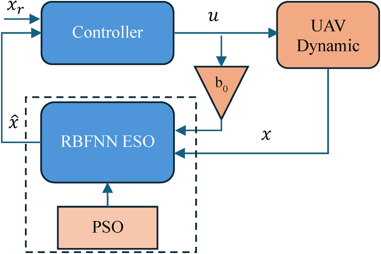
Structure of RBF neural network ESO. (Where
As illustrated in Figure 1, the RBFNN-based disturbance observer adopts an Extended State Observer (ESO) framework. The ESO expands the system state by introducing an additional state variable that represent the aggregated disturbance, which encompasses external disturbances, measurement noise, and model uncertainties. The observer estimates this disturbance state and compensates it within the control input to mitigate its impact. The RBF network's capability to approximate arbitrary nonlinear functions is leveraged, with parameter optimization achieved through PSO, as denoted by the dashed box in Figure 1.
The neural network employed for disturbance estimation consists of three layers: the input layer, hidden layer, and output layer, as illustrated in Figure 2.
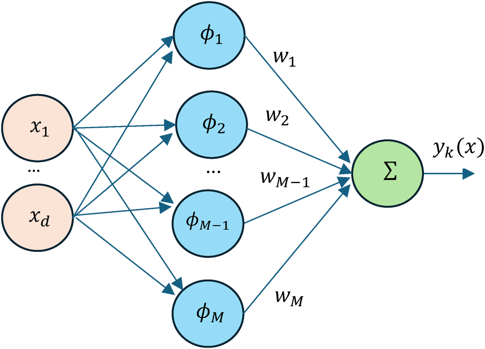
RBFNN network structure. (Where
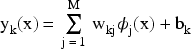
The output of the RBFNN can be expressed as:
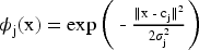
There are various types of radial basis functions, among which the Gaussian function is commonly used, as shown in equation (2):
For N training samples, the output of the RBF neural network can be expressed in matrix form:

The parameters of the Gaussian function, including the center C, width
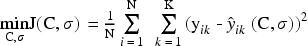
The purpose of RBFNN optimization is to minimize the error in disturbance estimation. This can be achieved by selecting an appropriate objective function and minimizing it. Therefore, this paper uses the Mean Squared Error (MSE) of the network output as the objective function, which is minimized by selecting appropriate Gaussian function parameters, such as the center C, width
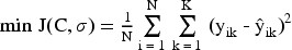
However, parameter selection is a time-consuming task. To obtain the optimal parameters, repeated test based on experience or experimental methods is usually required. Therefore, optimization algorithms are often employed to automatically find the optimal parameters. In the context of UAV disturbance estimation, disturbances vary randomly; thus, real-time parameter optimization using PSO is clearly infeasible. This is because PSO optimization demands a relatively long time and can only be implemented in an offline manner.
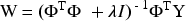
After the optimal
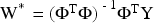
To prevent overfitting, a regularization parameter
In this paper, the focus is on the discussion in optimizing C and


The adaptive strategy described in equation (7) requires integration with control methods, for which sliding mode control has been adopted. As the primary focus of this paper remains on disturbance estimation, details regarding the controller design can be found in the previous work (Wei et al., 2025).
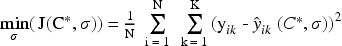
The PSO algorithm requires particles position vectors configuration based on the parameters to be optimized. In this study, since the parameters to be optimized are centers and widths, so the position vector of each particle can be defined as:

It is a vector to be optimized that contains M center points and widths. To optimize the vector, an appropriate fitness function must be selected. The objective of this study is to identify the optimal centers and widths that minimize the objective function of the RBF network. The adopted fitness function is:
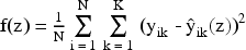
where Y denotes the output of the RBF network, and
Velocity update:

Position update:
The inertia weight serves as a critical parameter to balance exploration (global search) and exploitation (local search). Existing methods can be categorized into four types: constant, random, time-varying, and adaptive (Kessentini & Barchiesi, 2015). Based on performance comparisons from relevant literature and consideration of computational efficiency, this study adopts a linearly time-decreasing strategy (Shi & Eberhart, 1999), as expressed in equation (14).
Hybrid Optimization Strategy with K-Means Initialization
PSO is a heuristic optimization algorithm capable of locating optimal solutions through stochastic exploration. However, this random exploration wastes considerable time. Particles often start in data-sparse regions and need many iterations to reach dense areas, consuming excessive computational resources. To reduce the time required for optimal solution discovery, this study introduces a hybrid optimization strategy that integrates K-Means with PSO, thereby accelerating the identification of optimal activation function centers. By employing K-means clustering, the centers are initialized within regions that reflect the actual data distribution, rather than being randomly assigned. This allows PSO particles to initiate their search directly from promising areas, enabling the algorithm to focus on fine-tuning rather than coarse exploration. Consequently, the method better captures data characteristics and enhances the speed of convergence to the optimal solution.
The initialization of centers using K-Means clustering proceeds as follows:
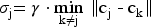
After determining the centers, a common approach is to calculate the widths based on the distances between centers, as shown in equation (16).
The K-means clustering algorithm first provides an initial estimate of the RBFNN basis function centers
In terms of the intrinsic characteristics of the optimization problem, the joint optimization of the RBFNN basis function centers
Firstly, the objective function
Secondly,
Two-Stage Optimization Strategy
To address the non-convex optimization challenge in jointly optimizing RBFNN basis function centers C and widths σ, traditional single-stage approaches are prone to local optima and cannot guarantee disturbance estimation accuracy. This paper proposes a nested two-stage optimization framework, which essentially implements a hierarchical strategy of “dimensionality reduction followed by fine-tuning”. The method decomposes the original
Stage 1: Joint Global Optimization of
and
Based on K-Means Initialization
To prevent the PSO algorithm from converging to data-sparse regions during random initialization, the first stage uses K-Means clustering results as initial anchors. By minimizing the sum of squared distances from samples to cluster centers through K-Means, initial center values
The core objective of the first stage is to jointly optimize C and
To achieve efficient joint optimization, the following key design strategies are implemented in this stage. Building upon the vector structure established in equation (9), the parameter C and

This vector has a dimension of
To enhance global search capability, the inertia weight
To prevent parameters from losing physical significance, hard constraints are imposed on
The core objective of the first stage is “center-dominated joint coarse adjustment”. Through coordinated optimization of
In this stage, the complexity of K-Means is
Although the first stage yields an optimized center When When
Therefore, selecting an appropriate width range is crucial to ensure that the basis function responses adequately cover the input samples while preserving sufficient discriminative capability, thereby enhancing the network's generalization performance. Next, the second stage reduces the optimization dimensionality to an M-dimensional single-variable problem by fixing
This design decouples the interaction between C and
The vector dimensionality is reduced from
The objective of this stage's width optimization is to determine the optimal width that minimizes estimation error. While the fitness function and inertia weight strategy remain consistent with the first stage, the following adjustments are made to specific PSO parameters to achieve precise width tuning: the learning factors are modified to
In summary, the proposed two-stage optimization algorithm for RBFNN parameters with K-Means initialization not only escapes local optima but also reduces computational complexity. The overall algorithm flow is illustrated in Figure 3. After initializing the centers using K-means clustering, the two-stage optimization process determines the optimal centers and width parameters. Subsequently, the RBFNN output and corresponding weight values are computed to achieve accurate estimation of the input disturbances.
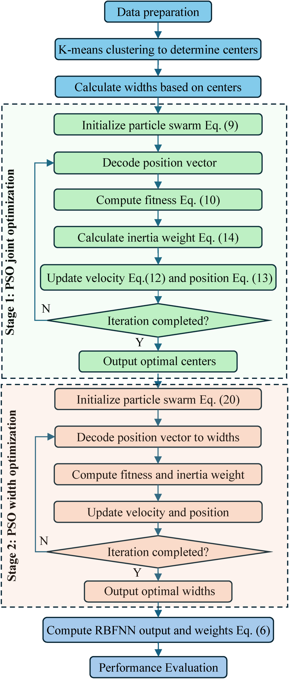
Flowchart of the K-means-based two-stage PSO algorithm for RBFNN parameter optimization.
Hyperparameter sensitivity is inherently linked to algorithm convergence, meaning parameter selection must ensure the algorithm's stability. For the PSO algorithm, the selectable hyperparameters include inertia weight w and learning parameters

The following is the proof :
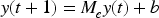
PSO algorithm's velocity update formula is showed as equation (12). Assume the algorithm enters stagnation:
Velocity update becomes:

Position update becomes:

where
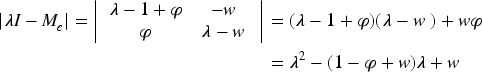
Characteristic equation:

According to the Schur stability condition, the necessary and sufficient condition for the roots of
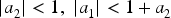
Here
Therefore, if the above three conditions (equation (28), equation (29), equation (30)) are satisfied, the steady-state convergence of the algorithm can be ensured, which is the basis for the selection of PSO hyperparameters. In the second stage of the algorithm, selection of


The simulation experiments were performed using Python, with the programming environment and basic parameters detailed in Tables 1 and 2.
PSO Parameter Settings.
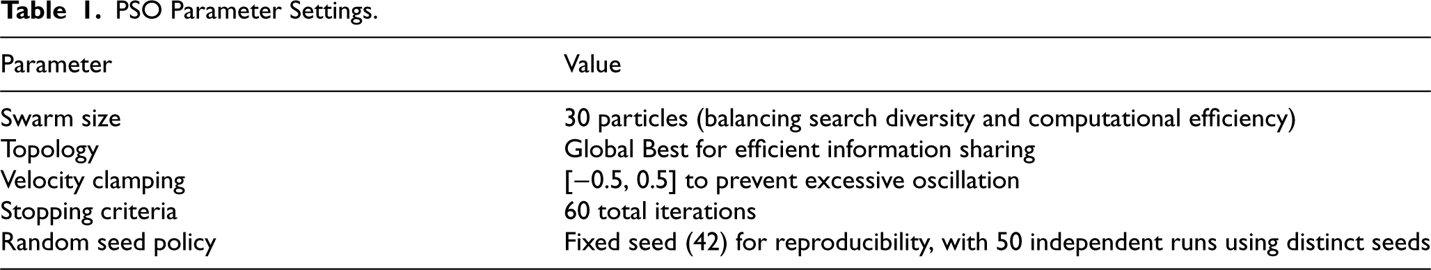
PSO Parameter Settings.
Implementation Details.

To fully validate the effectiveness of the proposed algorithm, experiments were conducted under three different scenarios. Scenario 1 uses a synthetic dataset for validation. Scenario 2 employs the Dryden wind disturbance model for validation. Scenario 3 uses real UAV flight data for validation.
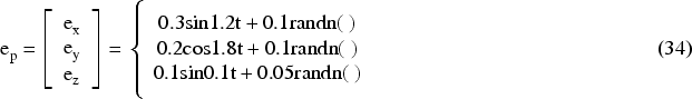
The objective of this study is to optimize RBFNN parameters for disturbance estimation. To evaluate the optimization performance, simulated data were generated by incorporating random disturbances to establish input-output relationships, as refer to in Li et al. (2024); Chang et al. (2024). The input consists of 12-dimensional state variables, specifically: 3-axis attitude errors (

The attitude errors in the input data are generated using equation (23), where 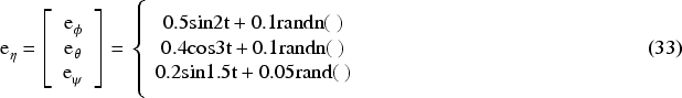
The disturbance forces F and disturbance moments M are given by equation (25) and equation (26), respectively, where the noise perturbation is generated using random 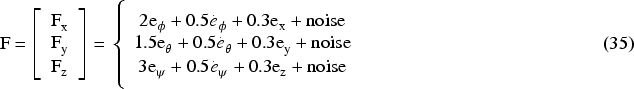
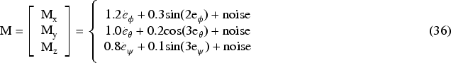
A partial view of the simulated data source is shown in Figure 4.
Simulated data (partial).
To validate the performance of the proposed algorithm, three benchmark methods were compared. The first method initializes centers using K-Means clustering (MacQueen, 1967) and calculates widths based on these centers, denoted as KMeans-RBFNN. The second comparative approach builds upon K-Means by incorporating a PSO optimization algorithm (Clerc & Kennedy, 2002), which employs a single-stage optimization strategy and is referred as PSO-RBFNN. The third algorithm enhances PSO by modifying the inertia weight based on cumulative binomial probability (Agrawal & Tripathi, 2021) following K-Means initialization, termed CPBPSO-RBFNN. The performance comparison of these algorithms is illustrated in Figures 5–11 and summarized in Table 3.
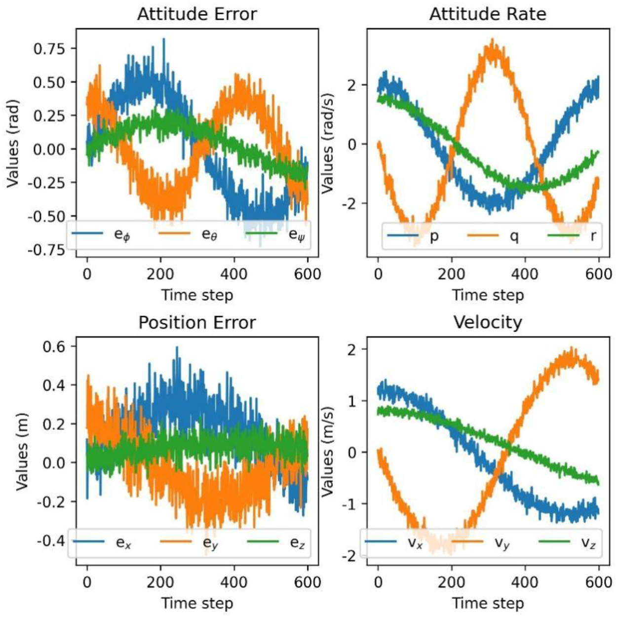
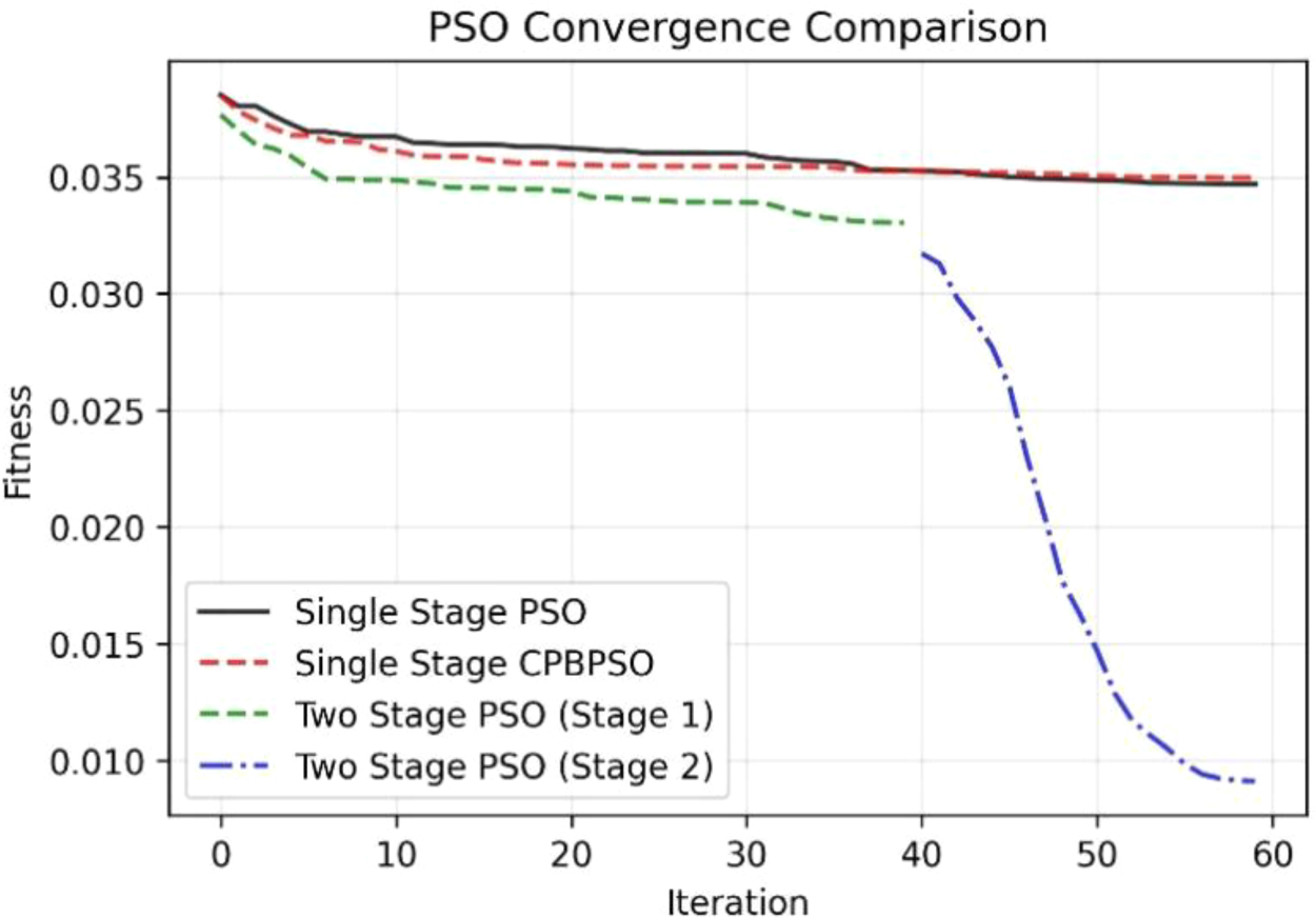
Comparison of PSO algorithm convergence.
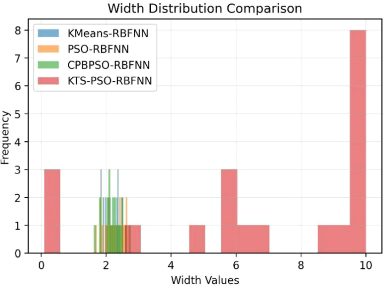
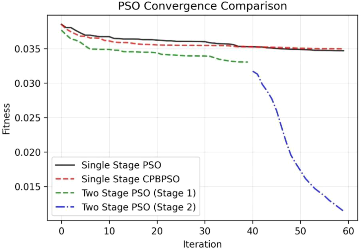
Width distributions of different algorithms.
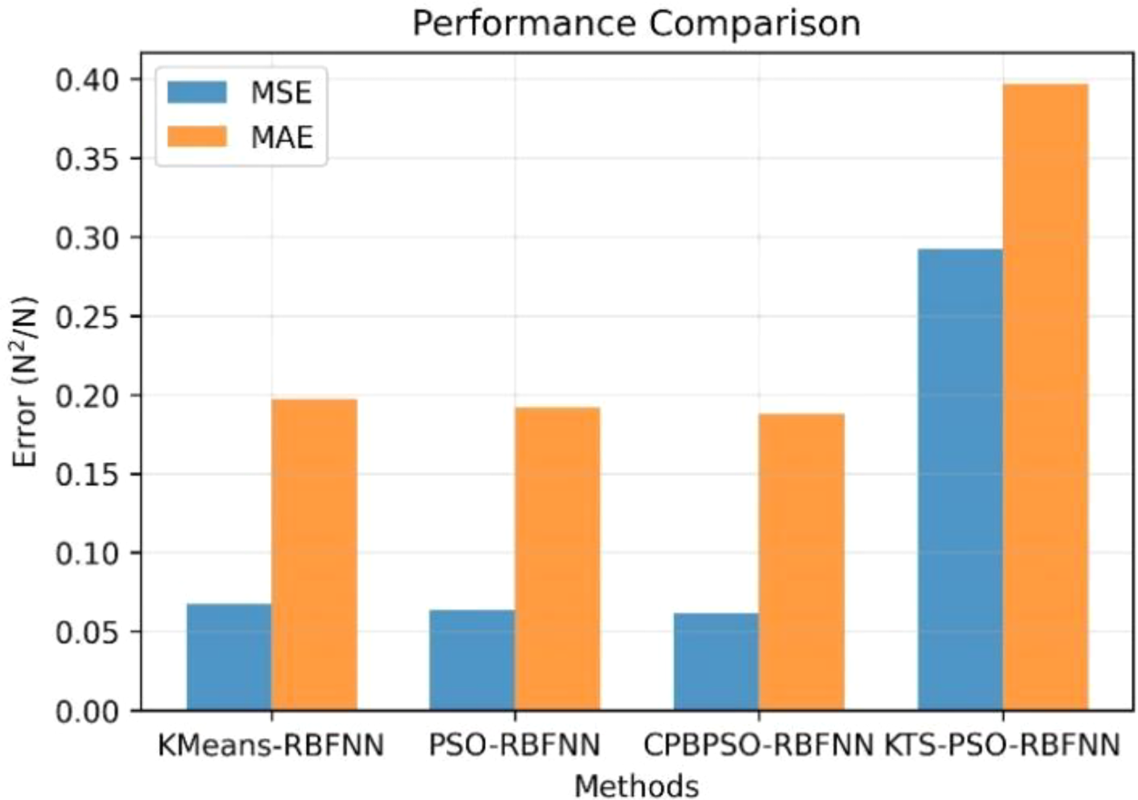
Prediction error comparison of different algorithms.
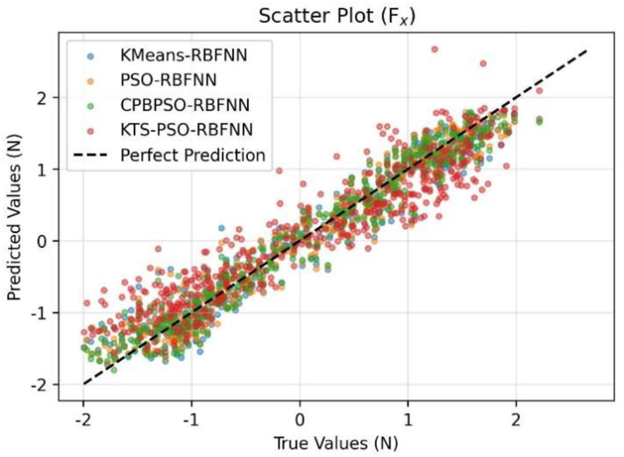
Comparison of disturbance force predictions by different algorithms.
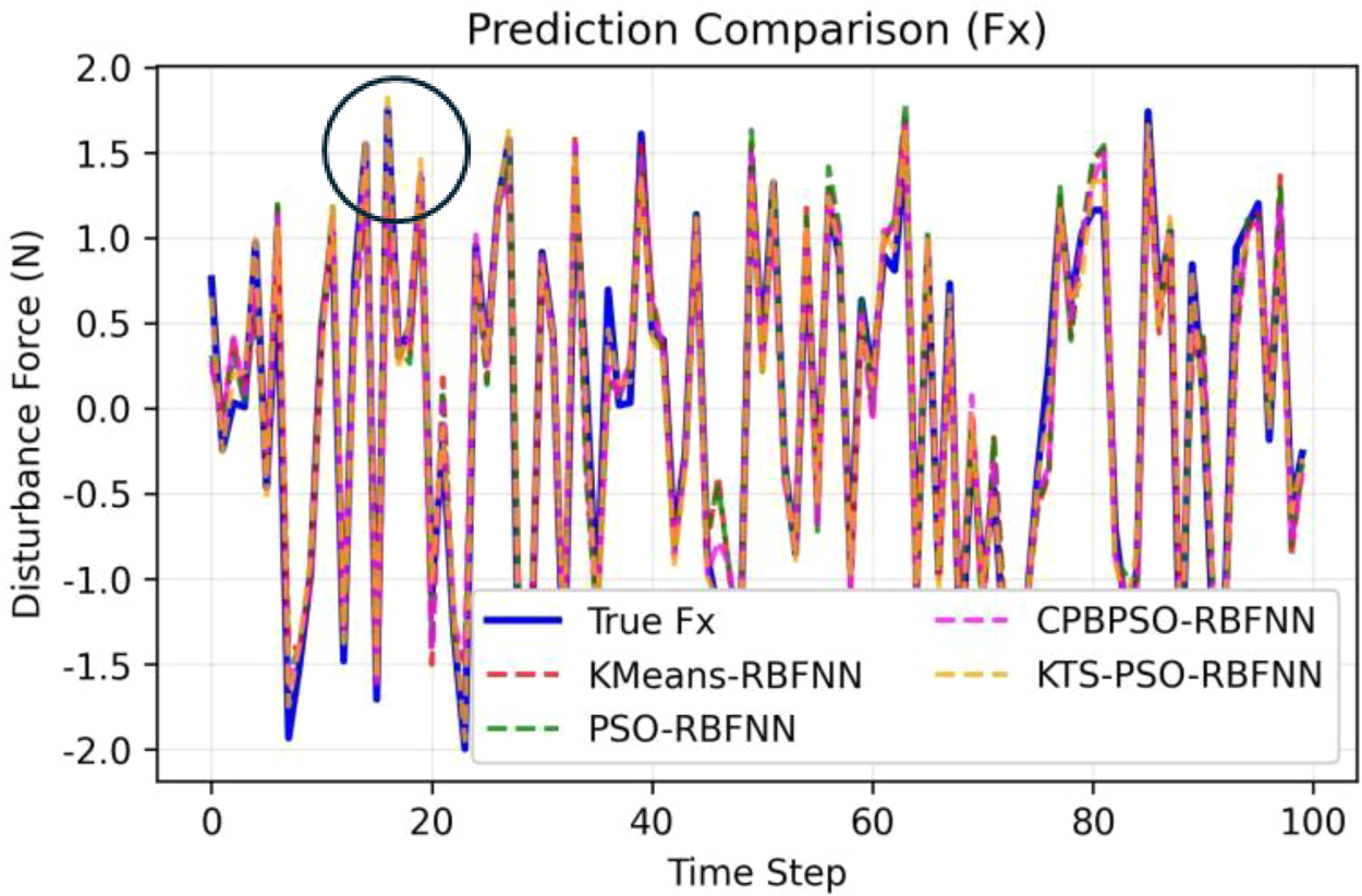
Comparison of predicted disturbance force outputs by different algorithms.
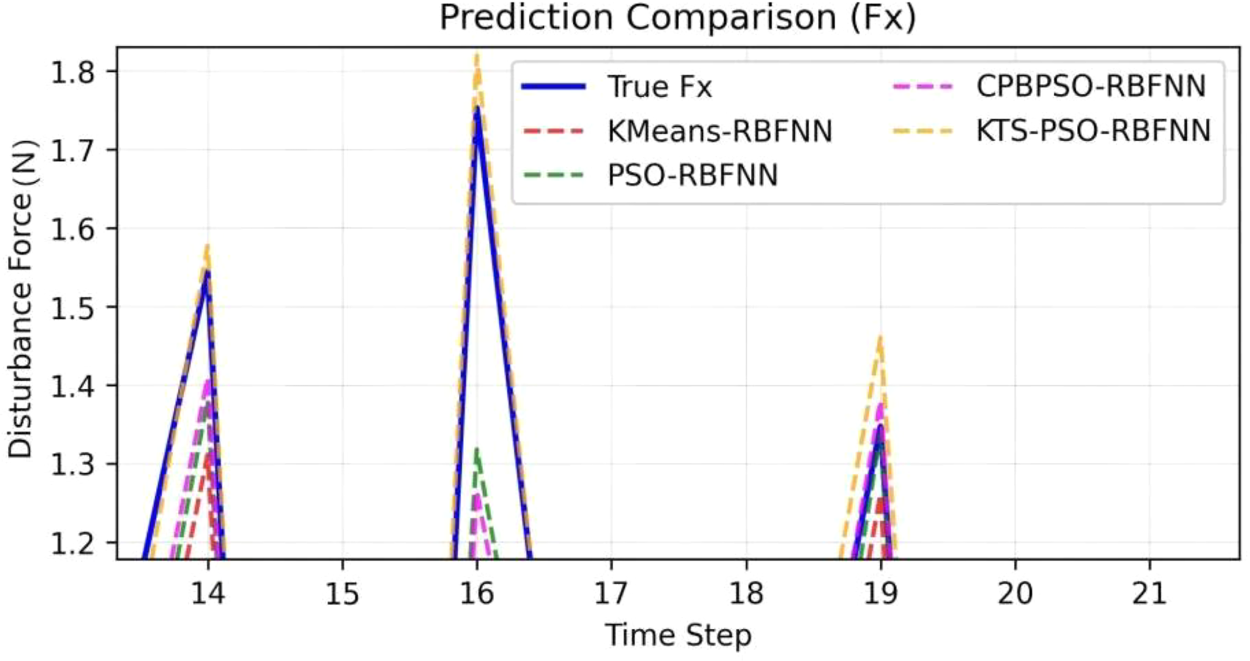
Magnified view of disturbance force predictions.
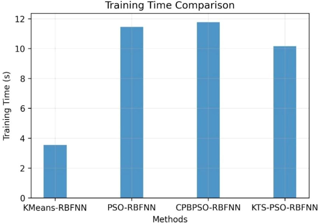
Training time comparison of different algorithms.
Error Comparison Data of Different Algorithms.
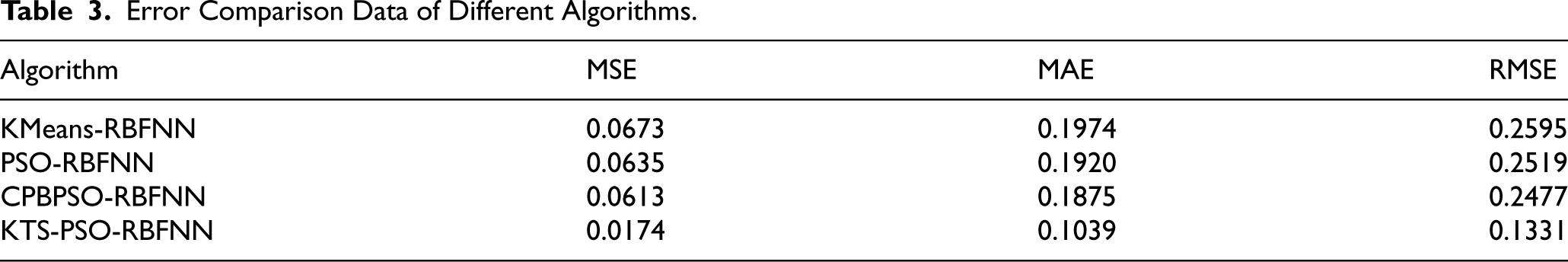
Figure 5 demonstrates the convergence behavior of the fitness functions across different algorithms. It can be observed that both the single-stage PSO and the first stage of the proposed algorithm exhibit significantly slowed convergence after approximately 5 iterations. In contrast, the two-stage PSO algorithm shows rapid fitness reduction at the beginning of the second stage, descending swiftly from the first-stage baseline until final convergence.
Figure 6 displays the width values obtained by the three algorithms. The KTS-PSO-RBFNN algorithm only shows the width distribution from the second stage, as its first-stage width distribution is identical to PSO-RBFNN. The figure reveals that the width values of KMeans-RBFNN and PSO-RBFNN are relatively concentrated, varying approximately between 1.5 and 2.8. This concentration suggests a suboptimal state, though not necessarily the global optimum. In contrast, the proposed two-stage optimization algorithm (KTS-PSO-RBFNN) exhibits a broader width distribution value, spanning the constrained range of 0.1 to 10 as shown in the figure. Such a wide distribution facilitates escape from suboptimum and promotes broader exploration of the search space, thereby increasing the likelihood of attaining superior optimal solutions. This observation is consistent with the fitness value trends as shown in Figure 5.
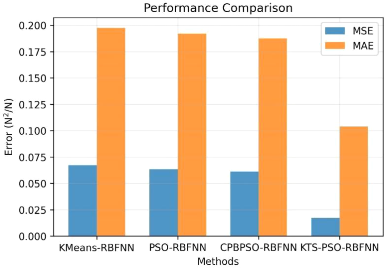
Figure 7 presents a comparison of prediction errors across different algorithms. The results indicate that PSO-RBFNN algorithm shows only marginal improvement over KMeans-RBFNN, with minimal reduction in error values. In contrast, the KTS-PSO-RBFNN algorithm demonstrates a substantial decrease in prediction errors. Specific numerical values provided in Table 3 reveal that KTS-PSO-RBFNN achieves the most significant reduction in MSE, decreasing by approximately 74.2%, 72.6%, and 71.6% compared to the other methods. Similarly, reductions of 44% to 48% are observed in Mean Absolute Error (MAE) and RMSE values, highlighting the remarkable performance advantage of the proposed KTS-PSO-RBFNN approach.
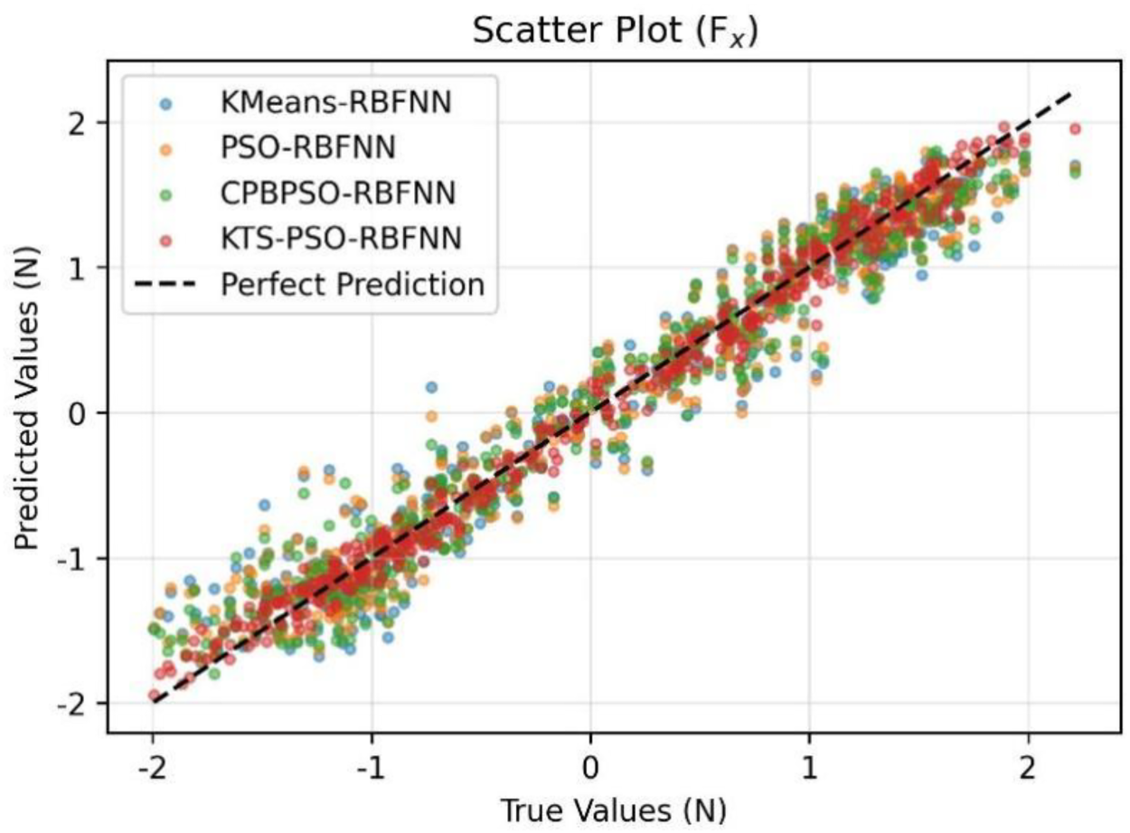
Figure 8 presents a scatter plot comparing the predicted disturbance force
Figure 11 illustrates the training time required by different algorithms. Although the KMeans-RBFNN algorithm exhibits the shortest time, it does not specify the number of iterations and is therefore not directly comparable. Among the remaining three algorithms, all of which employ 60 iterative computations, the KTS-PSO-RBFNN method demonstrates the shortest training time under identical conditions. It is noteworthy that even with its two-stage optimization process—40 iterations in the first stage and 20 iterations in the second—the proposed method achieves not only the lowest computational time but also the smallest estimation error, highlighting its exceptional performance.
To further evaluate the performance of the proposed algorithm, it is compared with an Extended State Observer (ESO) based observer. The ESO algorithm is implemented following the approaches described in Han (2009) and tested under the same operating conditions. The prediction results presented in Figure 12 indicate that the ESO exhibits relatively large prediction errors.
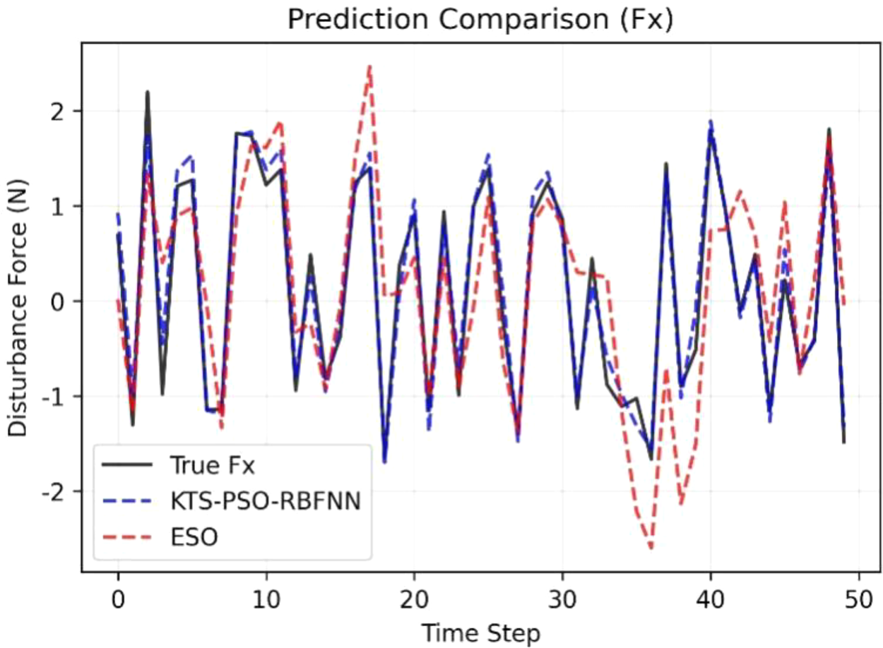
Comparison of prediction performance With ESO.
To provide a more comprehensive comparison of algorithm performance, 50 independent runs are conducted for each algorithm, with different random seeds used in each run to ensure randomness. The statistical results of these multiple-run comparative tests are summarized in the following tables and figures.
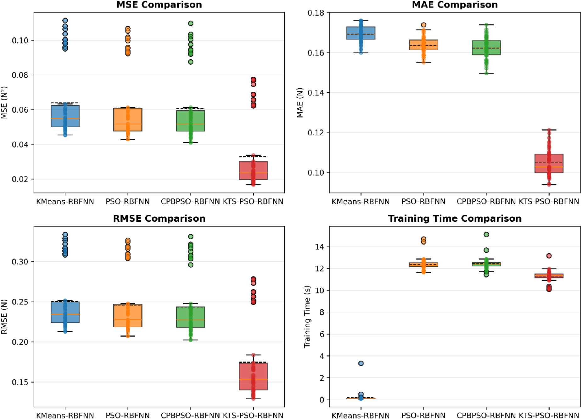
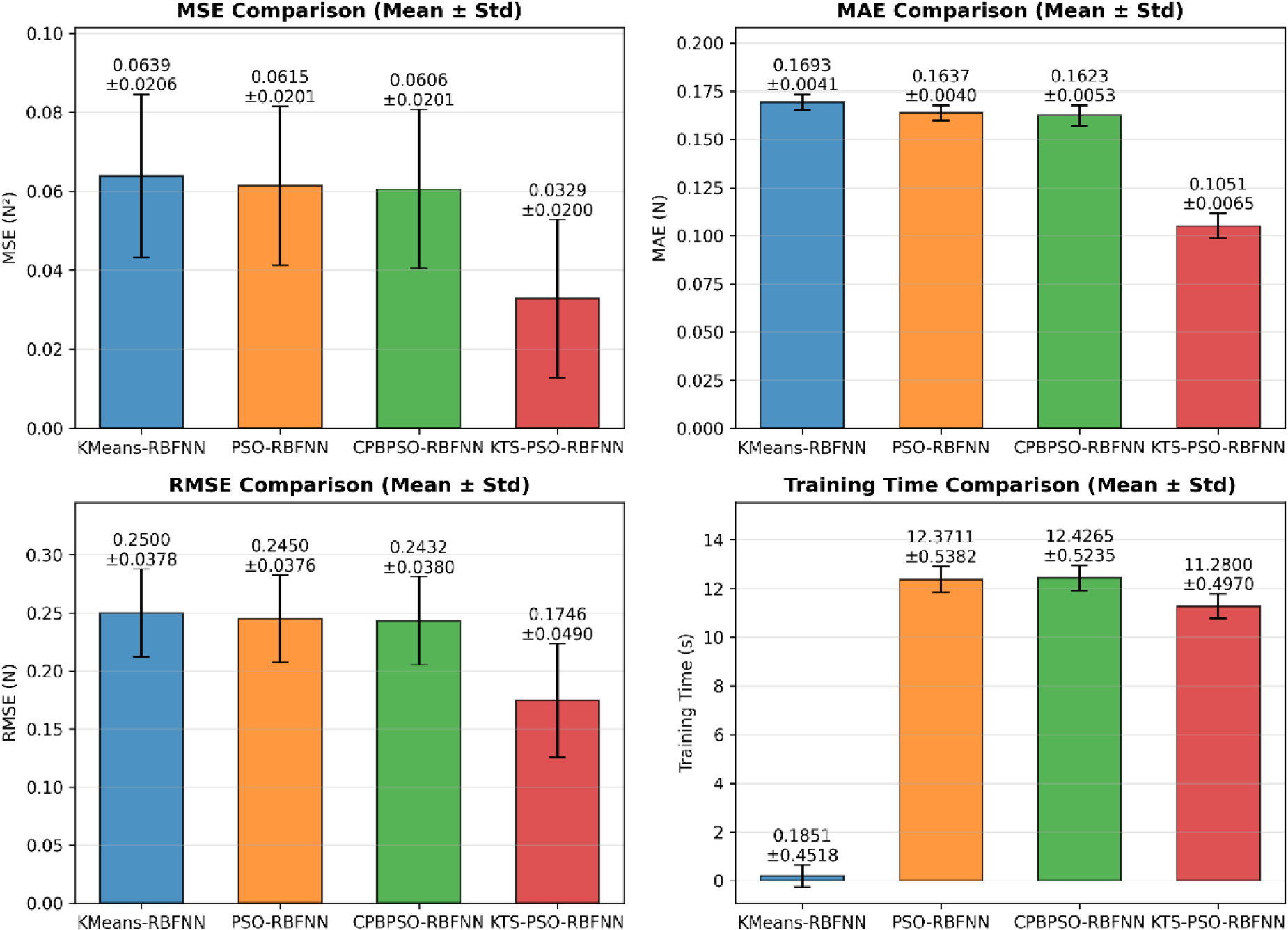
The statistical results presented in Figure 13 and Figure 14 demonstrate that even over 50 independent runs, the proposed algorithm maintains stable performance, with errors ranging between ±0.03 and ±0.08. According to the statistical data in Table 4, the MSE of KTS-PSO-RBFNN algorithm is reduced by 64.09%, 61.15%, and 61.00% compared to the KMeans-RBFNN, PSO-RBFNN, and CPBPSO-RBFNN algorithms, respectively. Although the reduction in MSE of the proposed algorithm is lower in a single run, it remains as the optimal among all compared algorithms. In conclusion, the proposed algorithm exhibits superior prediction performance over the other algorithms.
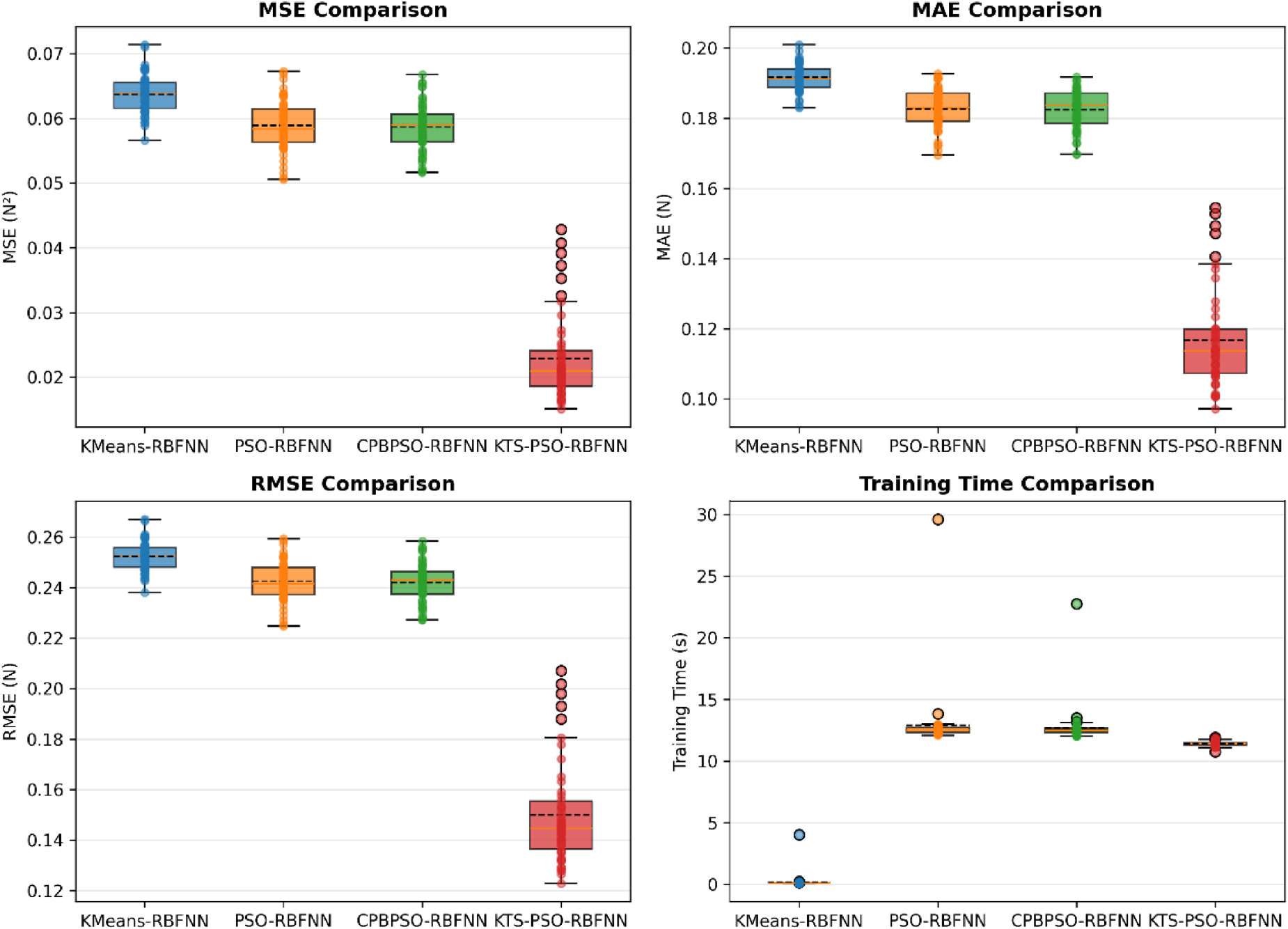
Statistical comparison of error and training time using boxplots.
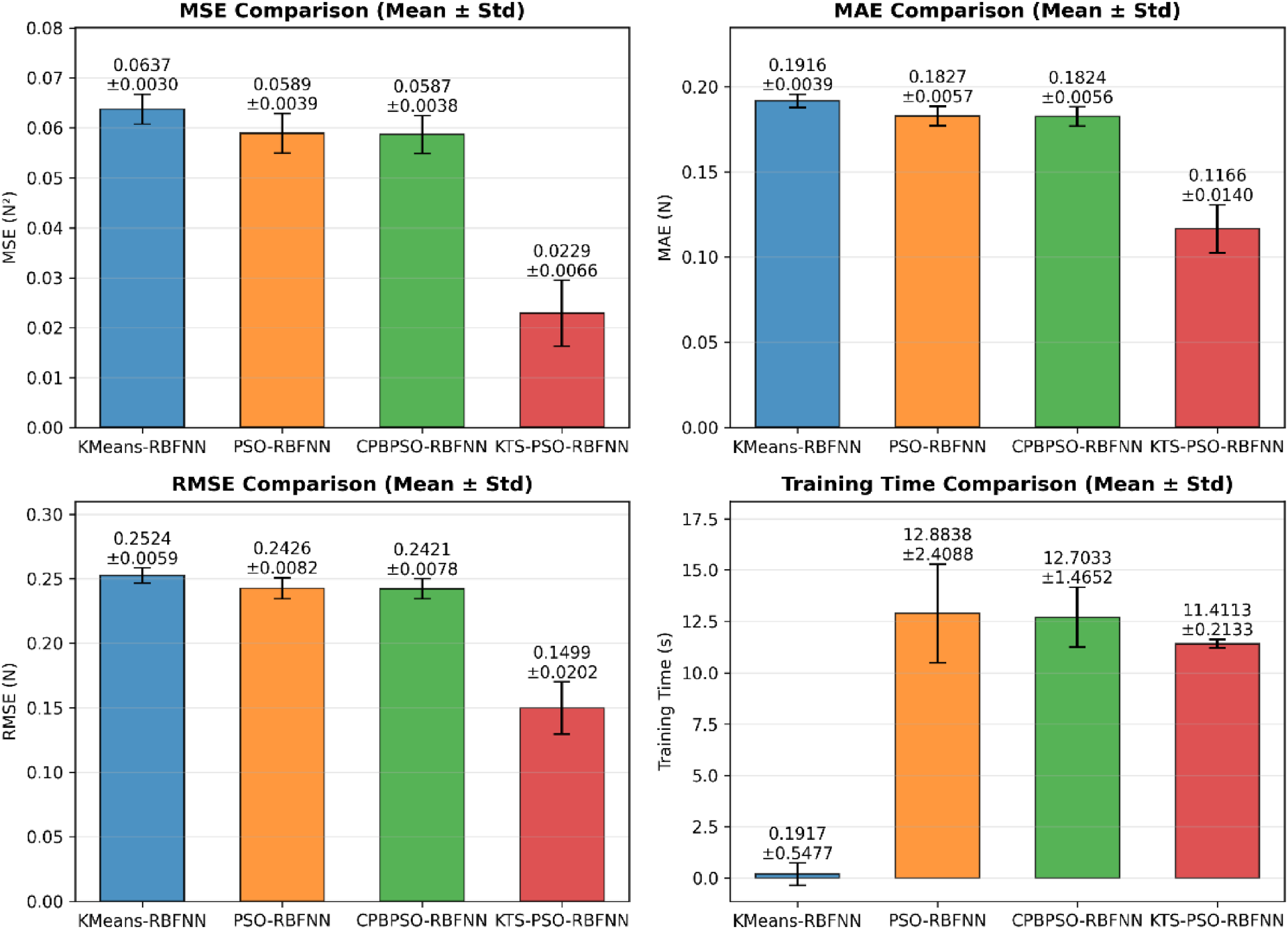
Statistical comparison of error and training time via bar charts.
Performance Comparison of Various Algorithms.
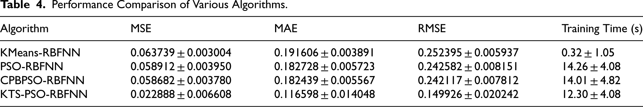
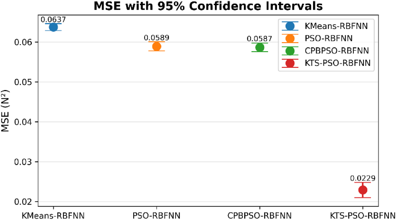
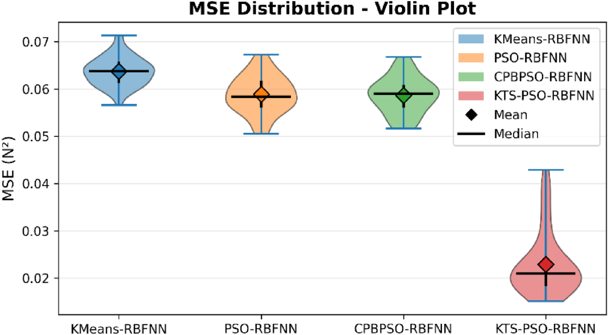
Figure 15 and Table 5 present the mean squared error (MSE) with 95% confidence intervals for four different algorithms: KMeans-RBFNN, PSO-RBFNN, CPBPSO-RBFNN, and the proposed KTS-PSO-RBFNN. As shown in the results, KTS-PSO-RBFNN algorithm achieves the lowest MSE of 0.0229, with a confidence interval ranging from 0.02099 to 0.02479. In contrast, the MSE values of the other three algorithms are significantly higher, all exceeding 0.058 with confidence intervals that do not overlap with the proposed method. This non-overlap of confidence intervals indicates a statistically significant improvement in prediction accuracy achieved by the KTS-PSO-RBFNN algorithm. The narrow confidence interval further suggests that the proposed method maintains consistent and reliable performance across multiple runs. The violin plot (Figure 16) of MSE distribution shows that the KTS-PSO-RBFNN algorithm exhibits a lower and more concentrated error distribution overall, while the baseline algorithms have wider error distributions with notably higher mean values, further validating the superior prediction accuracy and stability of the proposed method.
MSE error confidence intervals of various algorithms.
Distribution of MSE errors among various algorithms.
95% Confidence Interval of MSE Indicator.
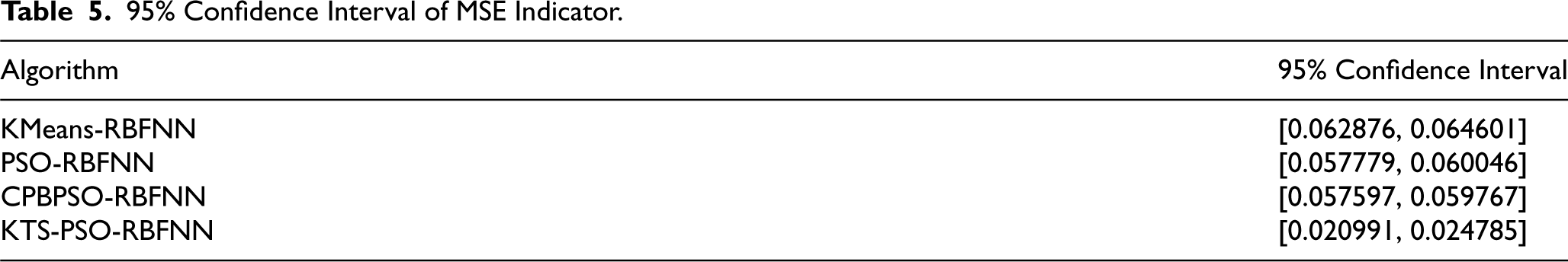
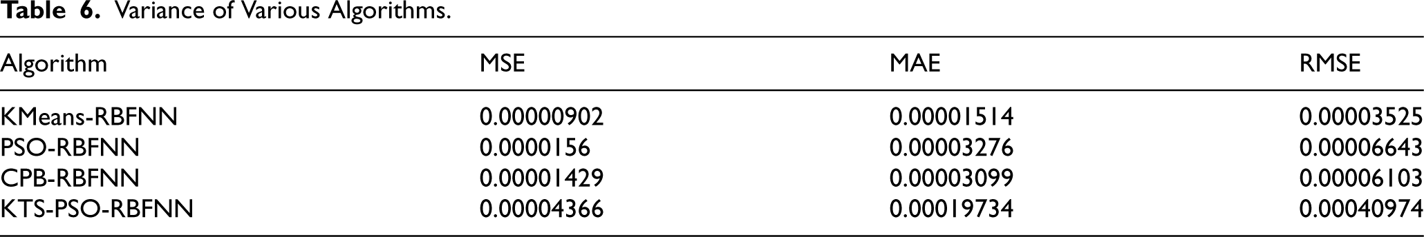
Table 6 presents the variance of the MSE, MAE, and RMSE metrics for all four algorithms over multiple runs. Variance serves as a key indicator of the stability and consistency of algorithmic performance—lower variance typically reflects more stable predictions across trials. It is worth noting that the proposed KTS-PSO-RBFNN algorithm, while achieving the lowest mean errors as demonstrated in previous results, exhibits the highest variance among all compared methods, with an MSE variance of 4.37 × 10⁻⁵. However, it is important to emphasize that this value remains well within an acceptable range. In absolute terms, a variance on the order of 10−5 is extremely small, indicating that even the “largest” fluctuations among runs are practically negligible. This suggests that although the proposed method shows slightly more variability than the others, its predictions remain highly consistent in absolute terms. The slight increase in variance is a reasonable trade-off for the substantial improvement in prediction accuracy achieved by the KTS-PSO-RBFNN algorithm. Overall, the proposed method successfully balances accuracy and stability, delivering superior mean performance while maintaining a level of variability that does not compromise its practical reliability.
Variance of Various Algorithms.
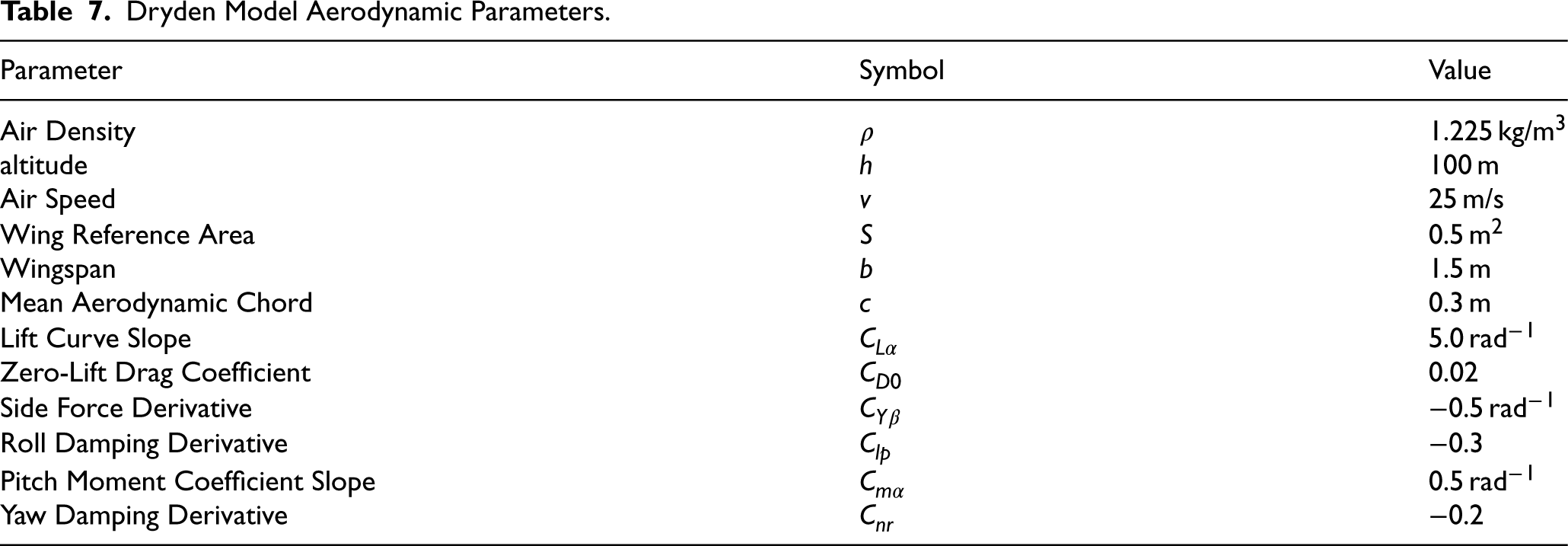
To evaluate the prediction performance under highly realistic disturbance conditions, the Dryden wind turbulence model was adopted. The implementation procedure of the model is as follows: First, the turbulence scale is calculated based on the flight altitude. Then, the turbulence intensity is determined according to both the turbulence intensity level (light/moderate/severe) and the altitude. Next, Gaussian white noise is transformed into colored noise through a filter, producing an output with the power spectral density of the Dryden model, thereby generating turbulence. Finally, the turbulence velocity is converted into forces and moments acting on the UAV to account for aerodynamic coupling. This method generates realistic wind disturbance data that conforms to statistical characteristics, providing a reliable test environment for disturbance estimation algorithms. The key parameters of the UAV and its aerodynamics are listed in Table 7. A total of 50 test runs were conducted using the Dryden wind turbulence model, and the statistical results are summarized in Table 8 and shown in Figures 17–20.
Statistical comparison of error and training time using boxplots under dryden wind disturbance model.
Statistical comparison of error and training time via bar charts under dryden wind disturbance model.
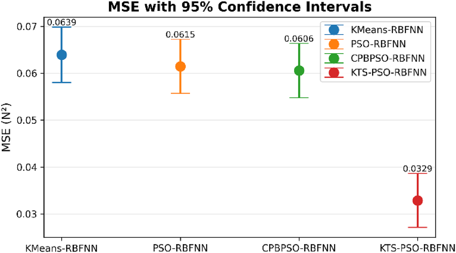
MSE error confidence intervals of various algorithms under dryden wind disturbance model.
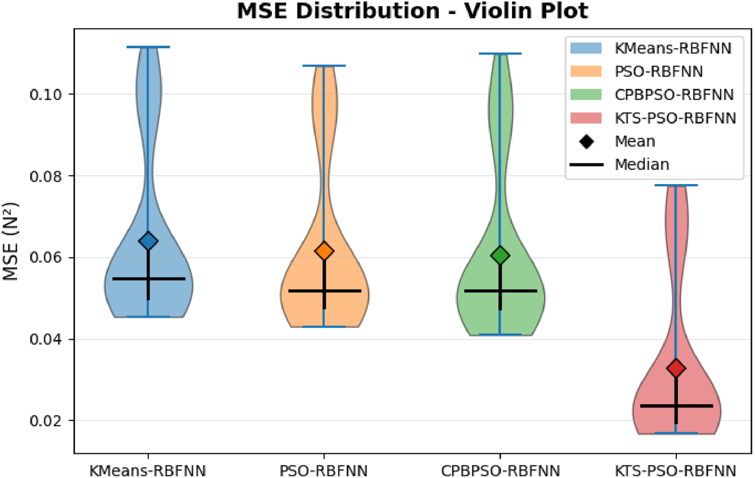
Distribution of MSE errors among various algorithms under dryden wind disturbance model.
Dryden Model Aerodynamic Parameters.
Error Comparison Under the Dryden Wind Disturbance Model.
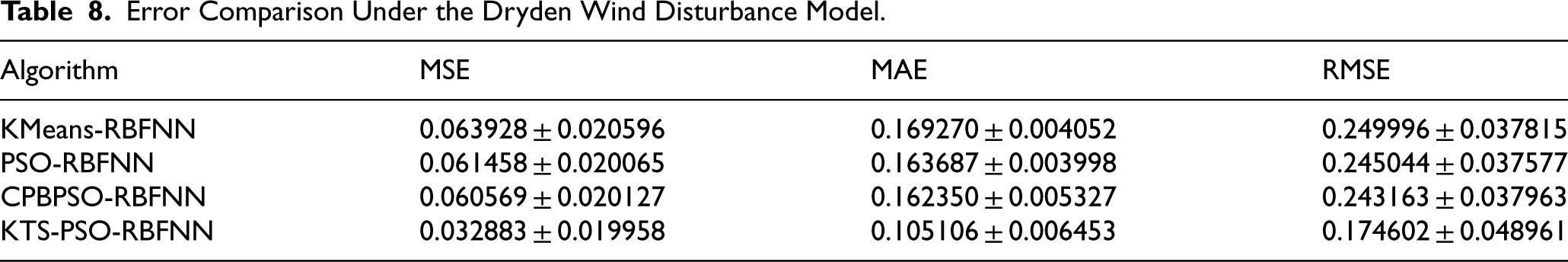
Table 8 presents the error metrics (MSE, MAE, and RMSE) of all four algorithms under the Dryden wind disturbance model over 50 test runs. The results are reported as mean ± standard deviation. As shown in the table, the proposed KTS-PSO-RBFNN algorithm achieves the lowest mean errors across all three metrics, with an MSE of 0.0329, an MAE of 0.1051, and an RMSE of 0.1746. In contrast, the three comparison algorithms—KMeans-RBFNN, PSO-RBFNN, and CPBPSO-RBFNN—exhibit significantly higher mean errors, with MSE values all exceeding 0.060, approximately twice of the proposed method. This indicates that the KTS-PSO-RBFNN algorithm substantially enhances prediction accuracy under realistic wind disturbance conditions.
The confidence interval plot further supports these findings. The 95% confidence intervals for the MSE of the proposed method are clearly separated and located below the other algorithms, demonstrating a statistically significant improvement in prediction performance. In terms of stability, the standard deviations of the proposed algorithm are comparable to the other methods, with MSE standard deviations around 0.02 across all algorithms. This suggests that despite the increased complexity of the wind disturbance model, the KTS-PSO-RBFNN algorithm remains consistent and maintains reliable performance across multiple runs.
From the results, although the MSE of KTS-PSO-RBFNN algorithm is slightly higher than the MSE obtained without the wind disturbance model, it is still reduced by 48.56%, 46.50%, and 45.71% compared to KMeans-RBFNN, PSO-RBFNN, and CPBPSO-RBFNN, respectively. Similarly, the MAE and RMSE values are also reduced by approximately 30%. These results demonstrate that even under realistic Dryden wind disturbance conditions, the KTS-PSO-RBFNN algorithm maintains lower prediction errors than the other algorithms, highlighting its robust prediction performance.
To further assess the robustness of the proposed algorithm across different disturbance conditions, two cross-validation experiments were designed. In the first experiment, all algorithms were trained on a synthetic dataset and subsequently tested on the wind disturbance dataset generated by the Dryden model. In the second experiment, the training and testing datasets were swapped: the algorithms were trained on the wind disturbance dataset and tested on the synthetic dataset.
This cross-validation setup aims to evaluate the generalization capability and robustness of each algorithm when exposed to data distributions different from those encountered during training. An algorithm with strong robustness is expected to maintain consistent prediction performance regardless of whether it is trained on synthetic data and tested on real-world-like wind disturbance data, or vice versa. The results of these experiments provide insight into how well each method adapts to unseen disturbance patterns and whether the proposed KTS-PSO-RBFNN algorithm retains its superiority under such cross-domain conditions.
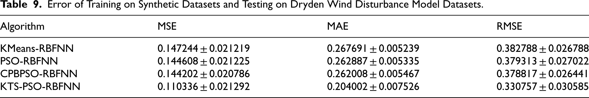
Table 9 presents the results when all algorithms were trained on synthetic datasets and tested on the Dryden wind disturbance model datasets. Table 10 shows the results of the reverse experiment, where those algorithms were trained on the Dryden wind disturbance datasets and tested on synthetic datasets.
Error of Training on Synthetic Datasets and Testing on Dryden Wind Disturbance Model Datasets.
Error of Training on Synthetic Datasets and Testing on Dryden Wind Disturbance Model Datasets.
Error of Training on Dryden Wind Disturbance Model Datasets and Testing on Synthetic Datasets.
As shown in Table 9, the proposed KTS-PSO-RBFNN algorithm achieves the lowest mean errors across all three metrics, with a MSE of 0.1103, MAE of 0.2040, and RMSE of 0.3308. In comparison, the three baseline algorithms—KMeans-RBFNN, PSO-RBFNN, and CPBPSO-RBFNN—exhibit substantially higher errors, with MSE values all exceeding 0.144, MAE values above 0.262, and RMSE values around 0.379. This represents a MSE reduction of approximately 23.5% to 25.1% for the proposed method relative to the baselines, demonstrating its superior generalization from ideal synthetic conditions to more realistic wind disturbance scenarios.
In terms of stability, the standard deviations of the proposed algorithm are comparable to those of the baseline methods, with MSE standard deviations all around 0.021. This indicates that the KTS-PSO-RBFNN maintains consistent performance across multiple runs even when tested on out-of-distribution data.
Experiment B: Training on Dryden Wind Disturbance Data, Testing on Synthetic Data
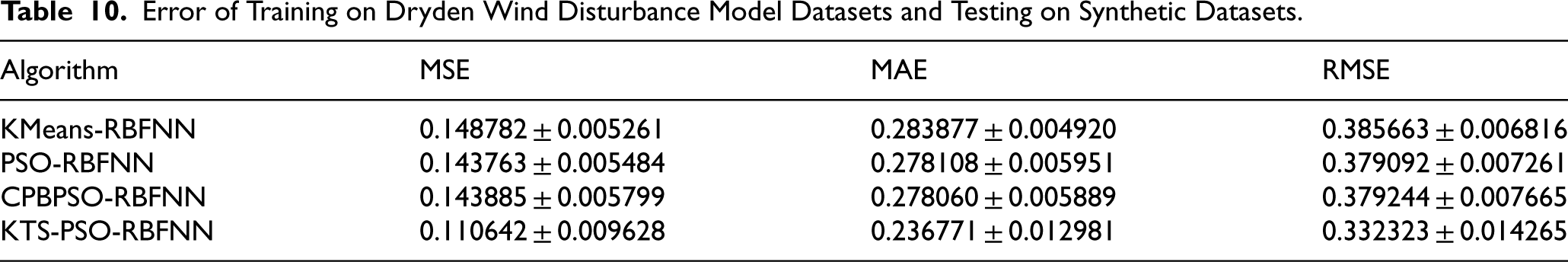
Table 10 presents the results of the reverse cross-validation experiment. Similarly, the KTS-PSO-RBFNN algorithm achieves the lowest errors, with MSE of 0.1106, MAE of 0.2368, and RMSE of 0.3323. The baseline algorithms show significantly higher errors, with MSE values around 0.144–0.149, MAE values around 0.278–0.284, and RMSE values around 0.379–0.386. The proposed method achieves a MSE reduction of approximately 23.2% to 25.7% compared to the baselines, confirming its strong adaptability when transitioning from realistic to synthetic data domains.
It is worth noting that the MAE of the proposed algorithm in Experiment B (0.2368) is slightly higher than in Experiment A (0.2040), suggesting that training on more complex wind disturbance data and testing on cleaner synthetic data presents a greater challenge for precise error magnitude prediction. Still, the proposed method outperforms all baselines by a substantial margin.
Cross-Validation Summary
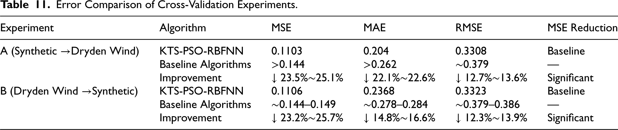
Across both cross-validation experiments, the KTS-PSO-RBFNN algorithm consistently achieves the lowest prediction errors, with MSE values around 0.110 in both directions, representing a reduction of over 23% compared to all baseline methods (Table 11). This consistent superiority under domain shifts demonstrates the strong robustness and generalization capability of the proposed algorithm. The standard deviations remain low and comparable across all methods, indicating that the performance gains are achieved without sacrificing stability. These results confirm that the KTS-PSO-RBFNN algorithm is highly adaptable to varying disturbance conditions and maintains its predictive advantage regardless of the training-testing domain configuration.
Error Comparison of Cross-Validation Experiments.
Error Comparison of Cross-Validation Experiments.
To make the experiments more realistic, we used the NeuroBEM datasets (Bauersfeld et al., 2021) for testing. This dataset provides real UAV flight data collected from onboard sensors and Vicon measurements. We selected a flight trajectory from the dataset, as shown in Figure 21. The second segment of the trajectory, which exhibits significant variations in attitude and position, was used as the input, while the predicted forces and moments from the datasets served as the output. Since the dataset does not provide attitude and error data, we obtained them using a fourth-order Butterworth low-pass filter. A total of 10,000 samples were collected, and 50 experimental runs were conducted. The comparative experimental results are presented in Table 12.
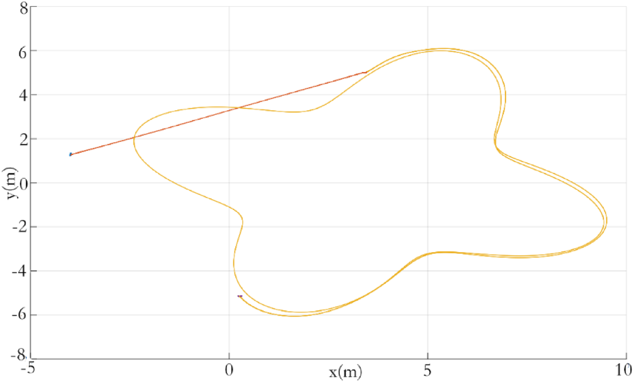
Flight trajectory.
Error of Training on NeuroBEM Datasets.
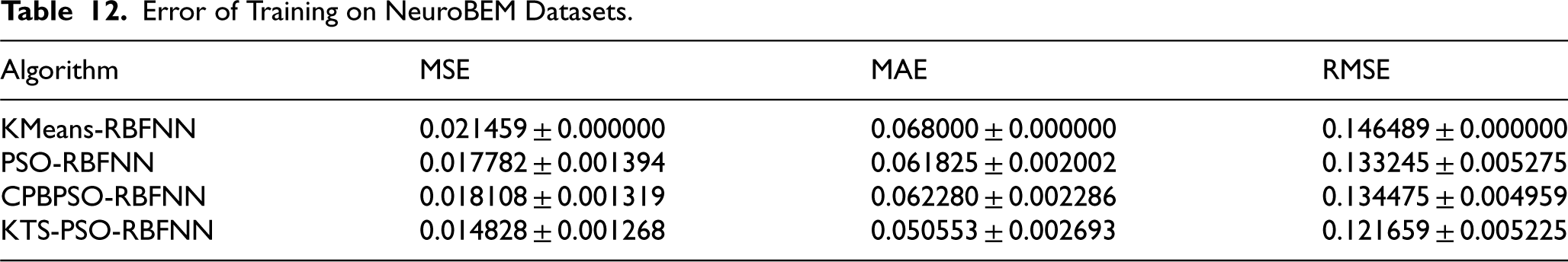
As shown in Table 12, the KTS-PSO-RBFNN algorithm also demonstrates excellent performance on the NeuroBEM datasets. All error metrics are the smallest among all compared algorithms, with MSE reduced by 16.61%, 18.11%, and 30.90% compared to the other algorithms, respectively. This confirms that even on real-world datasets, the proposed algorithm maintains superior prediction performance over the baseline methods.
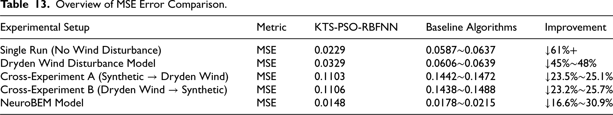
The overview of MSE error comparison is shown in Table 13. In summary, the proposed two-stage KTS-PSO-RBFNN algorithm demonstrates substantial improvements over conventional methods in both fitness convergence and prediction accuracy, highlighting its significant algorithmic advantages. This enhancement primarily stems from the two-stage PSO framework's ability to escape suboptimum. Building upon the joint optimization in the first stage, the second stage specifically refines the widths of RBFNN basis functions with greater precision, thereby substantially improving prediction accuracy.
Overview of MSE Error Comparison.
The experimental results presented above were obtained under constrained width conditions in the second stage. These constraints serve to prevent physically meaningless parameter values while avoiding underfitting caused by excessively large widths. Without such constraints, the PSO algorithm would conduct extensive searches to locate the global optimum. As shown in Figure 22, the width distribution without constraints ranges approximately from −85 to 75. Figure 23 provides a magnified view, revealing that this distribution encompasses the width ranges of KMeans-RBFNN, PSO-RBFNN, and CPBPSO-RBFNN while being substantially broader than their respective intervals.
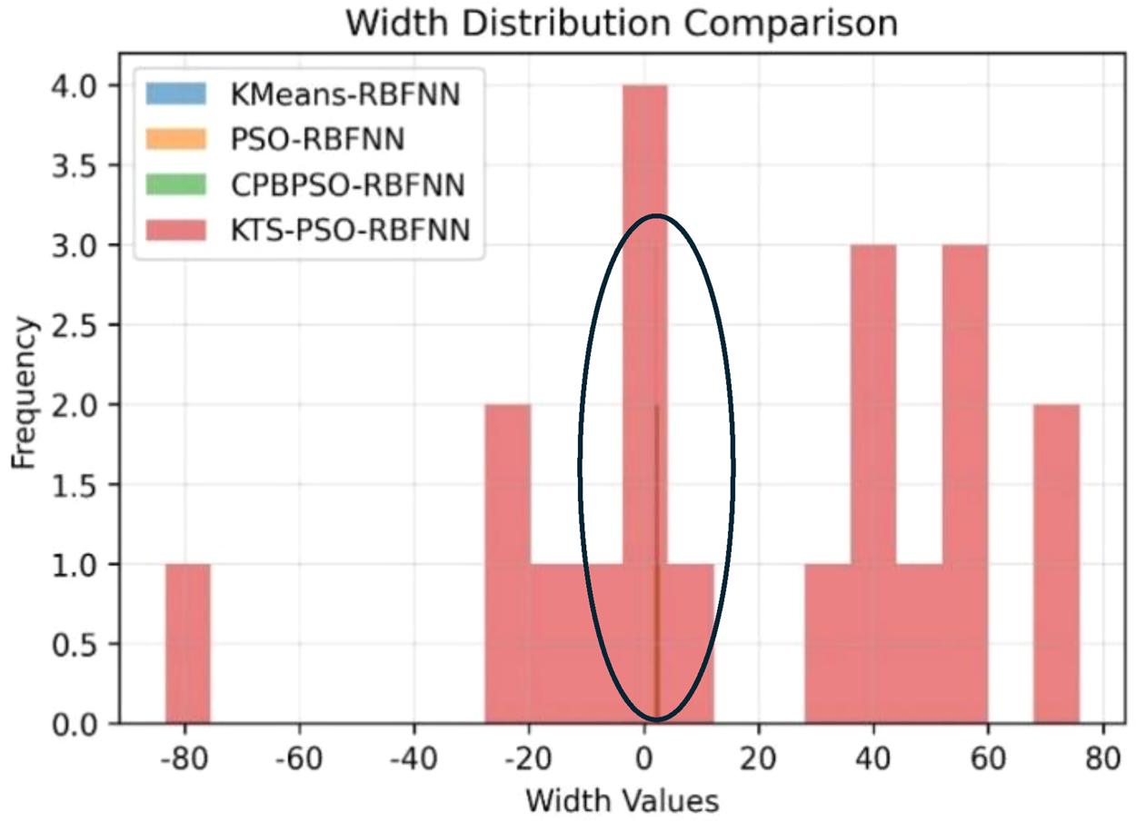
Width distribution without constraints.
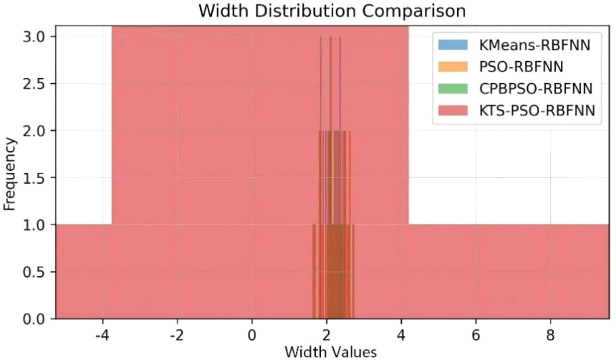
Magnified view of unconstrained width distribution.
Figure 24 compares the fitness convergence behaviors of the algorithms. It can be observed that without width constraints, the proposed algorithm achieves a further reduction in fitness value during the second stage until convergence, with the final fitness value being lower than that obtained under constrained conditions. This indicates that the absence of width constraints allows the PSO algorithm to explore more extensively and ultimately discover a superior solution with a minimized fitness value.
Comparison of PSO algorithm convergence without constraints.
Although a wide width distribution indicates strong global search capability, it does not translate to improved prediction accuracy. As demonstrated in Figure 25, the prediction error of the unconstrained KTS-PSO-RBFNN algorithm is slightly higher than the other three algorithms. Furthermore, the scatter plot of disturbance predictions generated by the RBFNN also exhibits poorer performance compared to other algorithms (as shown in Figure 26), demonstrating the necessity of imposing appropriate constraints during the second-stage width optimization.
Error comparison without constraints.
Disturbance force predictions caused by unconstrained width optimization.
Different width constraints yield varying optimization outcomes, making the selection of appropriate constraints crucial. Through targeted testing, it is observed that the relationship between width constraints and prediction error follows a curve with a distinct minimum, as illustrated in Figure 27. Within the evaluated constraint range of (1.5, ∞), the minimum error occurs at the maximum width constraint of
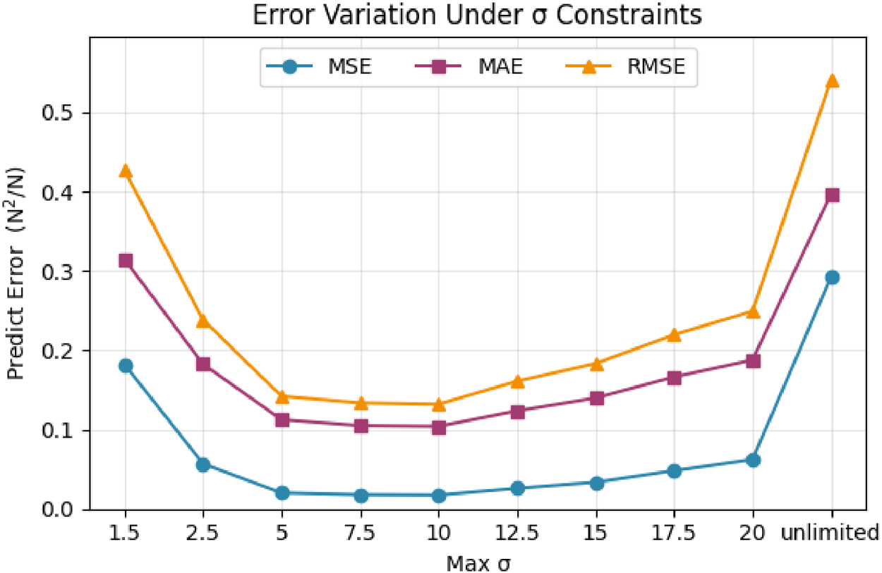
Error comparison under different constraints.
Regarding the computational latency issue, the average forward pass time of the RBFNN tested on the simulation computer is approximately 1 ms. When running on a UAV flight controller board, the computational latency is expected to be less than 10 ms, which is sufficient to meet the real-time disturbance prediction requirements. However, the PSO optimization takes about 12 s for 60 iterations. As shown in Figure 5, convergence can be achieved within 30 iterations, which still requires approximately 6 s of computation. This latency cannot satisfy real-time requirements. Therefore, the proposed two-stage PSO-based RBFNN parameter optimization can only be used as an offline optimization method at present.
This study proposes a K-Means-initialized two-stage particle swarm optimization RBF neural network (KTS-PSO-RBFNN) for disturbance estimation of UAVs operating in complex environments. The proposed method initializes the basis function centers and widths using K-Means clustering, allowing PSO particles to search from statistically dense regions of the data and thereby avoiding blind global search. Furthermore, the two-stage optimization strategy decouples the coupling effects among RBFNN parameters, effectively overcoming the inherent issues of premature convergence or entrapment in local optima.
The efficacy of the proposed algorithm was validated through three complementary experimental setups: synthetic data tests, Dryden wind disturbance simulations, and real flight dataset evaluations. In synthetic data tests, the proposed method reduces the mean square error (MSE) by over 60% compared to traditional methods. Under the more realistic Dryden wind disturbance model, the algorithm consistently maintains its performance advantage, achieving an MSE reduction of approximately 45%–48%. Cross-validation experiments further confirm the strong generalization capability of the proposed method, which consistently outperforms baseline approaches by more than 23% in MSE across various training–testing domain configurations. In real-world flight dataset experiments, the proposed algorithm also achieves a reduction in MSE of over 16.6% compared to other algorithms.
In summary, the proposed KTS-PSO-RBFNN algorithm effectively enhances disturbance prediction capability and provides a robust and reliable solution for UAV control systems operating in complex environments. Future work will focus on further optimizing the algorithm to reduce computational complexity and validating its effectiveness through hardware-in-the-loop (HIL) simulations.
Footnotes
Acknowledgements
The authors would like to thank Universiti Malaysia Sabah (UMS) for supporting this research. This work was also supported by the Grant from the Key Project of Fujian Polytechnic of Information Technology (Grant No.: YZDKJ25-02).
Ethical Considerations
Not applicable
Consent to Participate
Not applicable
Consent for Publication
Not applicable
Author Contributions
Longxin Wei contributed to methodology development and original draft preparation.
Kenneth Tze Kin Teo contributed to the formulation of overarching research goals and supervision of the research process.
Kit Guan Lim contributed to experimental design and implementation.
Min Keng Tan contributed to the development of the control algorithm.
Tianlei Wang contributed to experimental validation and formal analysis.
Yuto Lim contributed to manuscript review and revision.
Funding
The authors disclosed receipt of the following financial support for the research, authorship, and/or publication of this article: This work was supported by the Key Project of Fujian Polytechnic of Information Technology, (grant number YZDKJ25-02).
Declaration of Conflicting Interests
The authors declared no potential conflicts of interest with respect to the research, authorship, and/or publication of this article.