
Abstract
By addressing the operational and maintenance constraints of physical ground-based weather stations, this study proposes a deep learning (DL) framework for estimating reference evapotranspiration (ET0) by combining open-access climate services and remote sensing (RS) data. The proposed approach is benchmarked against traditional machine learning (ML) models, while multiple deep neural network (DNN) architectures are also evaluated, including multilayer perceptron (MLP), convolutional neural networks (CNNs), and recurrent neural networks (RNNs). Experiments conducted on three agricultural plots in southeastern Spain, representing contrasting meteorological conditions, demonstrate that RNNs achieve the best performance, with a coefficient of determination of R2 = 0.92. Furthermore, model interpretability was addressed using SHapley Additive exPlanations analysis, which confirmed the biophysical consistency of the predictions and identified land surface temperature as the primary driver of the model's estimations. A key contribution is the demonstration that infrastructure-free models trained solely on open-access satellite and climate data can match or even surpass conventional meteorology-based methods, providing a scalable solution for ET0 prediction. Based on a validation performed upon three agricultural plots in southeastern Spain, which represent contrasting semi-arid meteorological conditions, the framework showcases its potential applicability for global scalability by utilizing location-agnostic, open-access data. Moreover, the integration of crop coefficients enables accurate forecasting of daily irrigation demand. Overall, the proposed methodology illustrates the feasibility of artificial intelligence-driven irrigation management across diverse climates and highlights its potential to advance sustainable water use in agriculture.
Keywords
Introduction
Global food security and sustainable water management stand as the most pressing and urgent challenges of the 21st century (FAO 2021; Varzakas and Smaoui 2024). With a global population projected to approach ten billion, and facing the accelerating effects of climate change, the pressure on water resources has intensified, reaching a critical point. Prolonged droughts, extreme heatwaves, and erratic rainfall are transforming agricultural landscapes, threatening food production and the stability of rural economies. Agriculture, which consumes approximately 70% of the world's freshwater, is at the epicentre of this climate crisis, and faces significant challenges if innovative solutions are not adopted.
In this context, precision agriculture (PA) has emerged as a key strategy for mitigating these effects, with reference evapotranspiration (ET0) playing a central role in its effective implementation (Gyarmati and Mizik 2020). ET0 represents the rate of water loss through evaporation from the soil and transpiration from a hypothetical reference surface. This reference surface is a healthy, actively growing, and well-watered crop of grass with a uniform height of 12 cm (SIAR 2012). By standardizing this reference, ET0 provides a consistent measure of the climatic demand for water, independent of the specific crop type, its growth stage, or the soil conditions. Its precise measurement is vital for optimizing irrigation schedules, predicting crop water demand, and ensuring water efficiency in increasingly vulnerable agricultural systems (Youssef et al., 2024).
However, the estimation of ET0 faces a considerable obstacle: traditional methods, such as the Penman–Monteith equation (Allen et al., 1998), rely on a comprehensive set of meteorological parameters (solar radiation, wind speed, temperature, and relative humidity) that are obtained from ground-based weather stations. While these infrastructures are accurate, they are prohibitively expensive to install and maintain, and their distribution is often sparse and uneven, creating critical data gaps in arid, rural, and hard-to-reach regions (Yamaç, 2021). This limitation compromises the ability of farmers and resource managers to make informed decisions in a timely manner, which translates into inefficient water use, soil degradation, and reduced resilience to the water crisis. The need for a scalable, low-cost solution that does not depend on physical infrastructure is not just an advantage; it is an absolute necessity for global sustainability (Vaz et al., 2023).
To better contextualize our approach, it is essential to review the current landscape of computational models for ET0 estimation, particularly focusing on the trade-off between model complexity and data requirements.
To address these challenges, several authors have explored different computational approaches. Over the past few decades, the rapid expansion of artificial intelligence (AI) in PA has revolutionized how farmers manage key challenges like crop monitoring, pest control, and yield prediction. According to a literature survey, this technology helps farmers make better, more informed decisions for healthier crops (Sharma and Tripathi, 2021). The versatility of AI models is particularly valuable, as it allows them to be adapted for specific applications in diverse agricultural environments, from managing pests to improving irrigation (Sharma, 2021).
The integration of the Internet of Things (IoT) and Edge Computing has transformed real-time greenhouse monitoring by enabling on-site data processing and predictive analytics (Misra et al., 2022; Rayhana et al., 2020). AI-driven models, in combination with Big Data technologies, facilitate the complex analysis of greenhouse thermodynamics. This improves the prediction of temperature, humidity, and other key environmental factors (Escamilla-García et al., 2020).
In agricultural water management, accurate ET0 estimation is essential for optimizing irrigation efficiency. Traditionally, ET0 estimation has been based on empirical methods like the FAO-56 (Food and Agriculture Organization's Irrigation and Drainage Paper 56) Penman–Monteith equation, which requires a complete set of meteorological data. To overcome these data limitations, machine learning (ML) models emerged as a viable solution, showing promising results with fewer inputs. Early work by Yamaç (2021) and Vaz et al. (2022) demonstrated that models like Support Vector Machine (SVM) and Random Forest (RF) could achieve high accuracy with a reduced meteorological dataset, validating the effectiveness of AI in data-scarce environments. Furthermore, recent comparative studies have highlighted the potential of tree-based regression models, such as the M5 Tree, which provides a transparent and rule-based structure for ET0 estimation, often yielding competitive results compared to classical Artificial Neural Networks (ANNs) (Dadrasajirlou et al., 2022).
Building on the foundation of these neural architectures, deep learning (DL) has gained prominence in this field, demonstrating a superior capacity to model complex, non-linear relationships within large datasets. For example, Ravindran et al. (2021) have shown that Deep Neural Networks (DNNs) can outperform traditional ML models, yielding higher accuracy metrics. Specifically, this work validated a DNN with multiple dense layers, outperforming models such as decision tree (DT) or SVM. The literature has explored hybrid models that combine neural networks with metaheuristic optimization to further enhance performance, with models like the ANN Grey Wolf Optimization (ANN-GWO) reaching a coefficient of determination of up to R2 = 0.99 in the test phase (Khairan et al., 2023).
To further enhance performance and feature selection, the literature has explored hybrid models that combine ML with metaheuristic optimization. A prime illustration of this is the work by Ikram et al. (2023), which demonstrated how a hybrid Support Vector Regression (SVR) model, specifically one that combined Particle Swarm Optimization and GWO, reduced the Root Mean Square Error (RMSE) of the single SVR model by up to 32% in one of the studied stations. Similarly, regarding feature selection, Zhao et al. (2022) developed hybrid models such as Sparrow Search Algorithm (SSA) extreme learning machine (ELM) and Golden Eagle Optimization (GEO) ELM that achieved high accuracy with a coefficient of determination of R2 = 0.96. These models combine an ELM with a metaheuristic algorithm: the SSA and the GEO, respectively. More recent studies have used models like the XGBoost Regression model to optimize irrigation management in controlled environments, such as greenhouses (Ge et al., 2022).
Although previous studies have utilized XGBoost for its predictive accuracy, there is a lack of focus on model interpretability in infrastructure-free contexts. This study fills that gap by coupling XGBoost with SHapley Additive exPlanations (SHAP) to ensure that the estimated ET0 values are not only precise but also biophysically consistent.
Unlike existing hybrid models that prioritize architectural complexity to gain marginal precision using local data, our novelty lies in the validation of a scalable data-fusion framework. This approach addresses the ‘data-scarcity’ problem in regions where maintaining physical infrastructure is unfeasible. The benchmarking of convolutional neural networks (CNNs) and recurrent neural networks (RNNs) against open-source inputs reveals that the temporal-spatial capturing capabilities of DL are sufficient to match the performance of models that traditionally require on-site instrumentation.
Despite these significant advances, most models still rely on data from private weather stations, or have been validated over limited geographical scopes, which compromises their scalability and accessibility. This highlights a critical gap in the literature. Our study addresses this by proposing and validating a methodology that integrates multiple sources of open-access data. Consequently, a practical and replicable framework is offered by providing a systematic comparison between the capacity of RNNs and CNNs to process time-series and spatial data, respectively. Consequently, a practical and replicable framework is offered for precise ET0 estimation, demonstrating the ability of DL architectures to outperform ML techniques in a real-world application context.
To address this gap, our research proposes an innovative solution based on DL that integrates open-access data from climate services and remote sensing (RS). The primary objectives of this study are:
To develop a DL methodology for ET0 estimation that outperforms traditional ML models. To validate the feasibility of a scalable approach that does not require costly weather station infrastructure. To demonstrate the capacity of these models to support PA in diverse agroecological regions. To establish a replicable framework for integrating DL-based ET0 estimation into future AI-driven Decision Support Systems, enhancing the potential for data-informed irrigation strategies.
This work contributes to agricultural sustainability by offering a high-precision tool for water management. The remainder of this paper is organized as follows. The ‘Material and methods’ section details the proposed methodology, including data acquisition and model development. The ‘Results and discussion’ section presents the experimental results and a discussion of the findings. Finally, the ‘Conclusions and future work’ section concludes with the key findings and future research directions.
Material and methods
Reference evapotranspiration (ET0) calculation
The reference evapotranspiration (ET0) for each study plot was calculated using the Penman–Monteith combination method (Allen et al., 1998), widely recognized as the standard approach due to its robustness and applicability in diverse climatic conditions. The calculations were based on high-resolution, real-time meteorological data obtained from the Murcia Agricultural Information System (Sistema de Información Agraria de Murcia, SIAM) network of automated weather stations operated by the Murcia Institute for Agricultural and Environmental Research and Development (Instituto Murciano de Investigación y Desarrollo Agrario y Alimentario (IMIDA)). This high-quality, standardized dataset, computed according to FAO-56 guidelines (Katerji and Rana, 2014), serves as the ground truth for training and validating the DL models.
The full formula used is:
All the necessary meteorological components for the Penman–Monteith equation were calculated using the SIAM-IMIDA data. The net radiation

The remaining components were calculated as follows:
The The The
This rigorous methodological approach provides an accurate and reliable baseline for ET0 estimation, which is fundamental for validating the performance of the proposed DL models under the diverse climatic conditions of the study plots (SIAM and IMIDA, 2010).
Use case setting
Figure 1 shows the three agricultural plots selected for this study. They are all situated in the Region of Murcia (southeastern Spain); an area characterized by a semi-arid Mediterranean climate and chronic water scarcity.
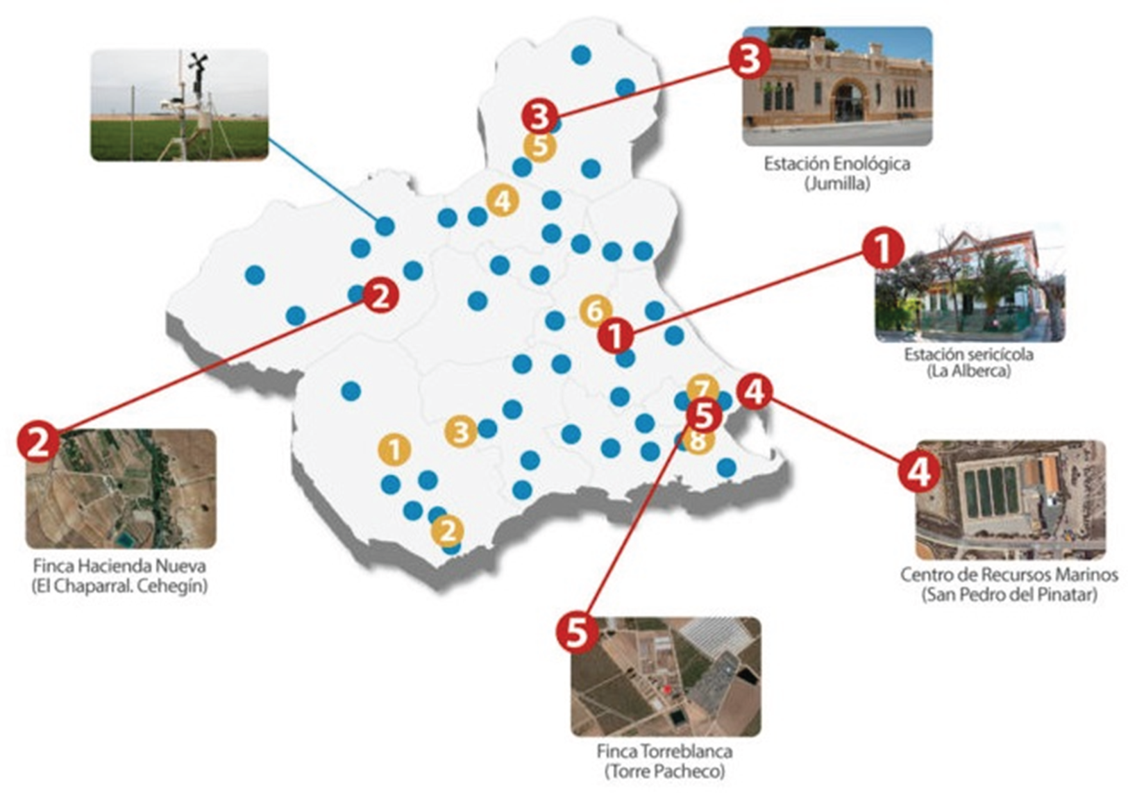
Geographic distribution of the study plots, focusing on the three selected locations: plot 1 (Estación Sericícola, labelled 1), plot 2 (Finca Torreblanca, labelled 5), and plot 3 (Finca Hacienda Nueva, labelled 2).
The plots were selected to capture spatial heterogeneity in microclimatic conditions, thereby enabling robust evaluation of climate-resilient irrigation and evapotranspiration modelling strategies.
The selection of southeastern Spain as a study area provides a rigorous testing ground due to its high-water stress and variability. Although this study focuses on this specific region, the methodology is inherently scalable to other geographical areas because it relies exclusively on global climate services and satellite products, bypassing the need for local instrumentation.
The meteorological baseline for these plots was obtained from the SIAM-IMIDA network (IMIDA, n.d.), which provides the standardized, quality-controlled variables used to compute ET0.
Data collection
Accurate estimation of ET0 in the studied semi-arid agricultural systems requires the integration of heterogeneous data sources capturing atmospheric, soil, and vegetation dynamics at appropriate spatial and temporal scales. To this end, a multi-source dataset was assembled for the three experimental plots (P1, P2, and P3). The data collection strategy was designed to combine ground-based measurements, gridded meteorological products, and satellite-derived variables, providing a comprehensive and temporally consistent representation of local hydroclimatic conditions. This integrative approach enables robust training and validation of data-driven models. It also supports irrigation management under variable climate scenarios. The main data sources incorporated in this study include the following:
Table 1 shows the four data sources considered in this study, covering the 2021–2024 period. CLMS provides 1931 daily records of LST, forming a consistent baseline for hydrological characterization. Although SSM data were initially available from this source, that variable was discarded due to a scarcity of values. Sentinel contributes 578 observations acquired every 2–5 days, including 19 spectral variables describing vegetation phenology and water dynamics at plot scale. OpenWeather offers 1048 daily meteorological records containing precipitation, temperature, humidity, and wind speed, capturing the atmospheric drivers of evapotranspiration. Finally, SIAM-IMIDA supplies 2123 daily measurements of ET0, which constitute the ground-truth benchmark for model calibration and validation.
Descriptive synthesis of the data sources.
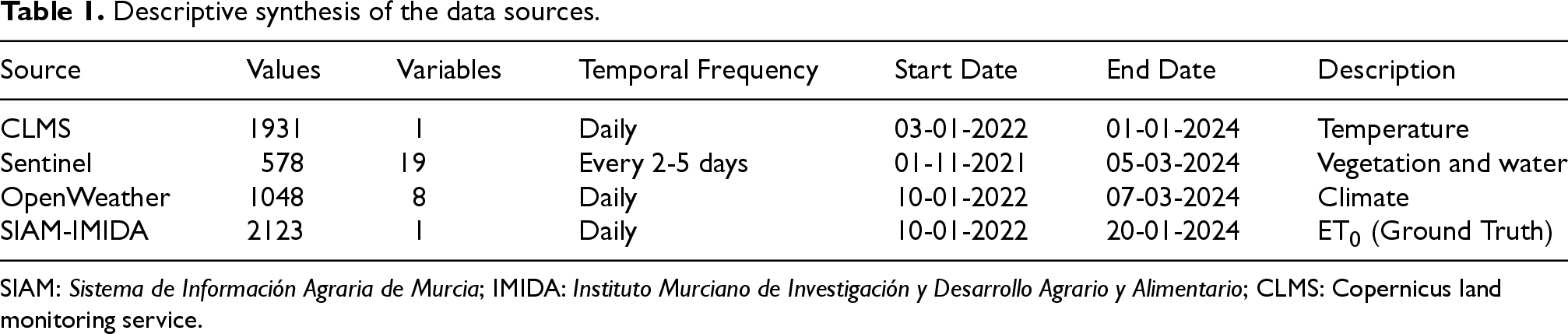
SIAM: Sistema de Información Agraria de Murcia; IMIDA: Instituto Murciano de Investigación y Desarrollo Agrario y Alimentario; CLMS: Copernicus land monitoring service.
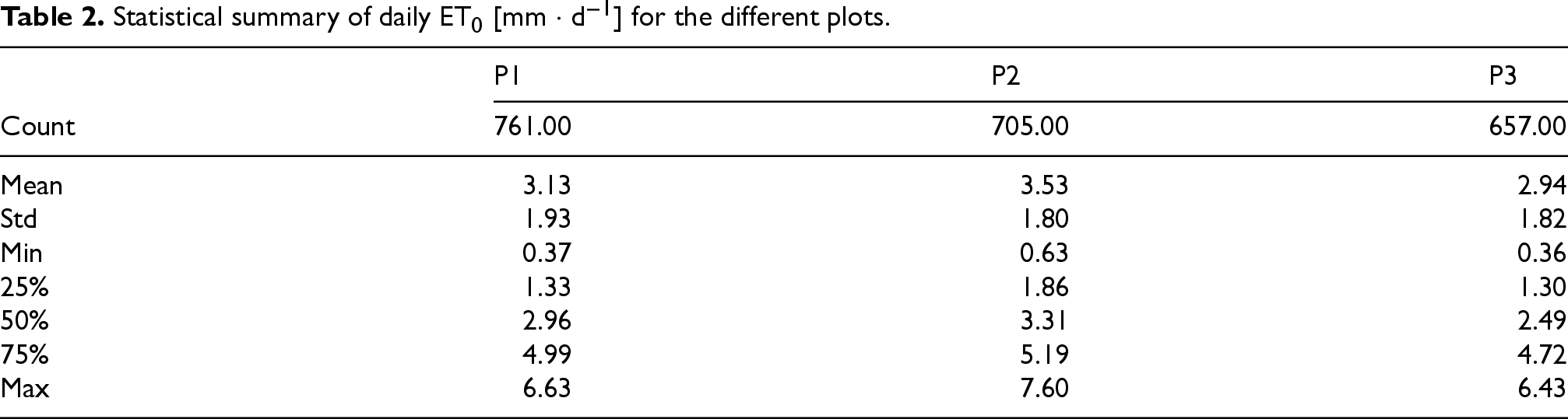
Building on this description, the statistical properties of the most relevant variables are subsequently examined, with a focus on ET0, to characterize the climatic conditions of the three experimental plots and assess their suitability for model training and evaluation.
Statistical summary of daily ET0 [mm · d−1] for the different plots.
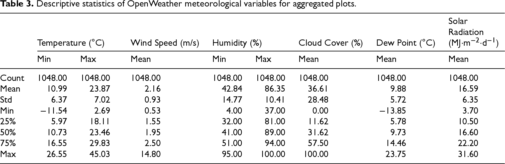
Descriptive statistics of OpenWeather meteorological variables for aggregated plots.
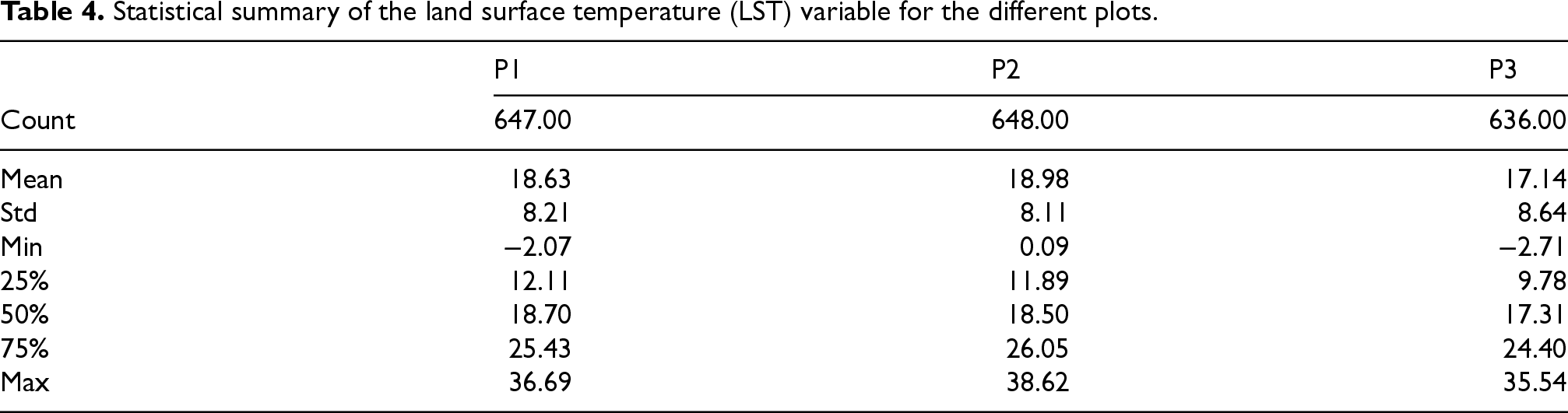
Statistical summary of the land surface temperature (LST) variable for the different plots.
Vegetation indices derived from Sentinel Hub imagery, including the NDVI, NDWI, Normalized Difference Moisture Index (NDMI), Green Normalized Difference Vegetation Index (GNDVI), Enhanced Vegetation Index (EVI), and Soil Adjusted Vegetation Index (SAVI), further characterize crop development and canopy moisture status. As summarized in Tables 5 and 6, NDVI values indicate moderate vegetation cover (mean ≈ 0.24), whereas negative NDWI values and low NDMI suggest periods of water stress or limited canopy moisture, both of which are relevant indicators for irrigation scheduling models.
Statistical summary of sentinel variables for aggregated plots (part 1).
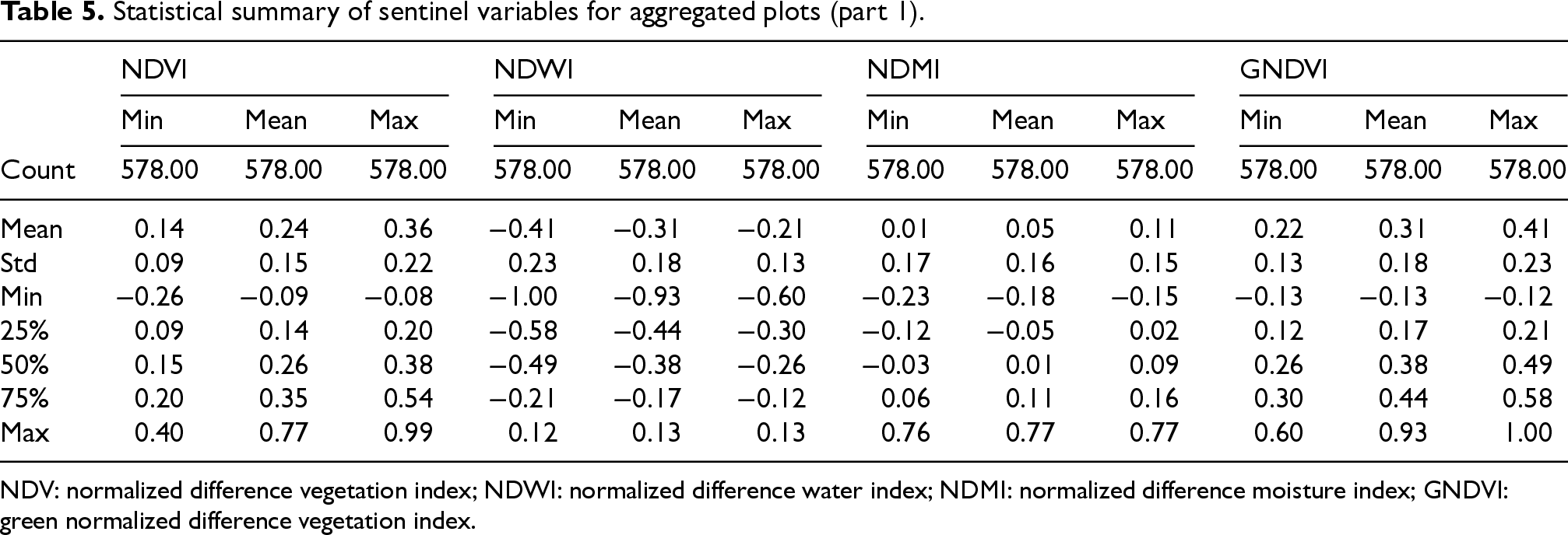
NDV: normalized difference vegetation index; NDWI: normalized difference water index; NDMI: normalized difference moisture index; GNDVI: green normalized difference vegetation index.
Statistical summary of sentinel variables for aggregated plots (part 2).
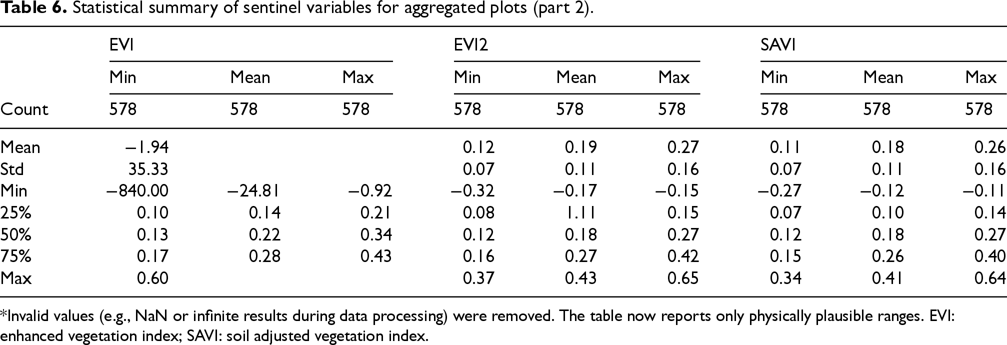
*Invalid values (e.g., NaN or infinite results during data processing) were removed. The table now reports only physically plausible ranges. EVI: enhanced vegetation index; SAVI: soil adjusted vegetation index.
Data processing
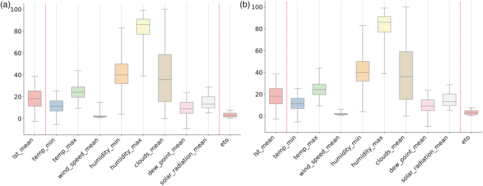
Boxplots of variables from CLMS, OpenWeather, and SIAM-IMIDA data sources before and after outlier removal. (a) Before preprocessing (raw data). (b) After preprocessing (cleaned data). SIAM: Sistema de Información Agraria de Murcia; IMIDA: Instituto Murciano de Investigación y Desarrollo Agrario y Alimentario; CLMS: Copernicus land monitoring service.
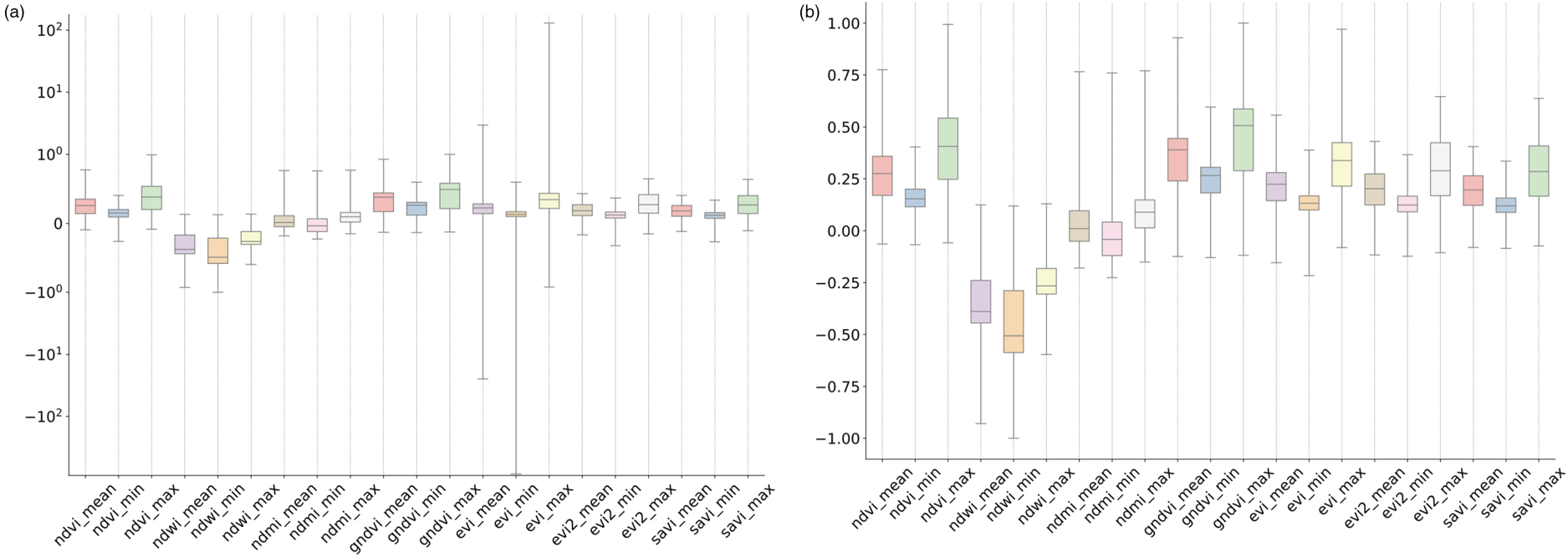
Boxplots of Sentinel-derived variables before and after outlier removal. (a) Before preprocessing (raw data). (b) After preprocessing (cleaned data).
The outlier removal strategy is based on percentile thresholds, specifically excluding values below the 10th percentile and above the 90th percentile. This aggressive filtering was a deliberate choice, adopted to counteract the high level of noise and potential contamination inherent in the integration of open-access RS and climate service data. Unlike the more traditional Interquartile Range (IQR) method, this approach provided a more deliberate and well-reasoned choice, ensuring that our models were not distorted by unrepresentative data while preserving the core data distribution. This decision was critical for improving the overall reliability of the trained models. This cleaning process not only improved the data's interpretability by centring variable distributions within typical ranges and reducing noise, but it also enhanced the reliability of the models trained in subsequent stages. The IQR is now more compact, reflecting representative values without distortion from extreme outliers. This adjustment facilitates pattern recognition, such as the moderate dispersion observed in indices like mean NDVI (ndvi\_mean) and mean NDWI (ndwi\_mean), compared to the lower variability in minimum SAVI (savi\_min) and minimum NDVI (ndvi\_min). Overall, this preprocessing enhances statistical reliability by reducing noise, leaving the data better suited for precise analyses and comparisons among indices.
Once the datasets had been cleaned and harmonized, we proceeded to evaluate multicollinearity to reduce redundancies and improve model stability, as described below.
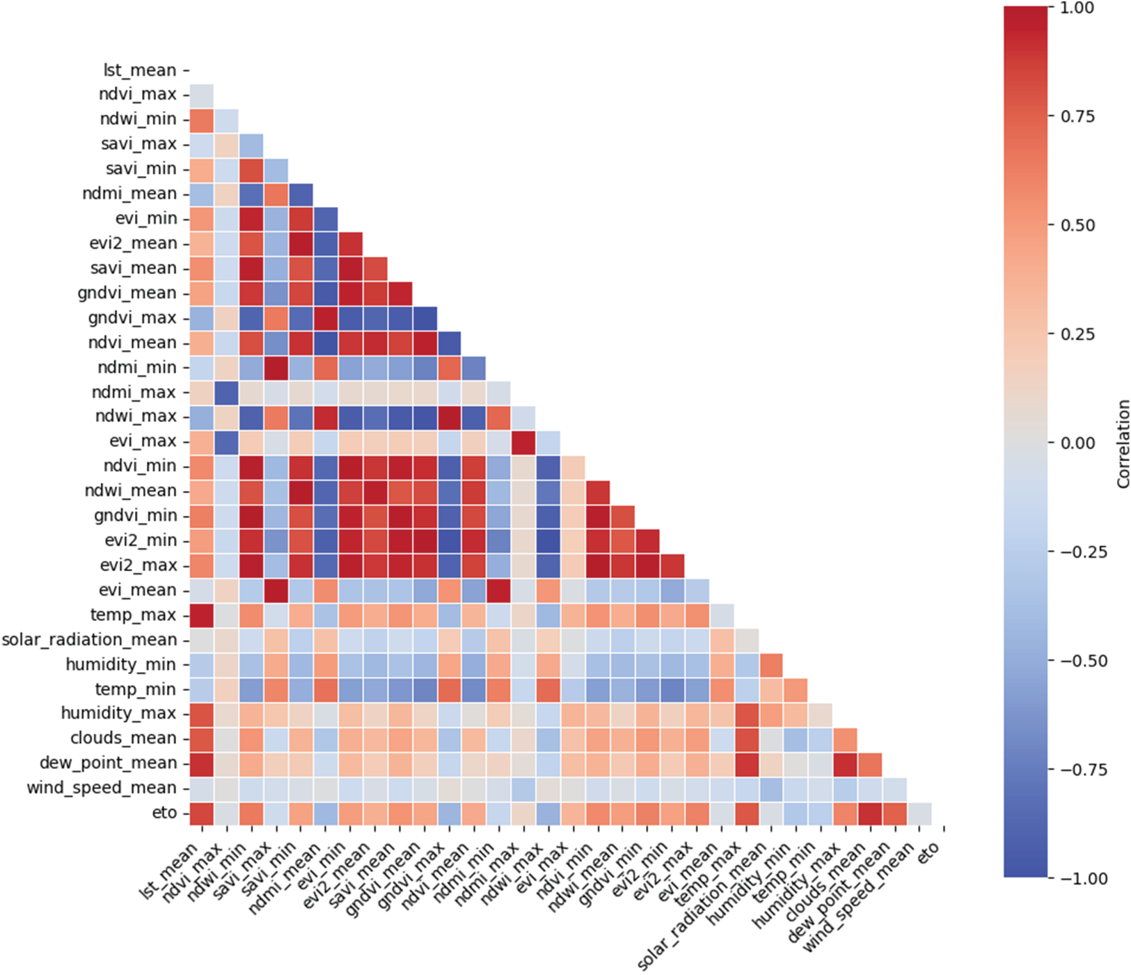
Correlation matrix for all variables.
Key observations include strong correlations among vegetation indices such as NDVI, EVI, and SAVI. This result is expected because all of them measure vegetation health and density. NDMI, which reflects soil and vegetation moisture, exhibits specific correlations with vegetation indices and climatic variables, highlighting its role in capturing broader environmental factors. Regarding climatic variables, maximum temperature and solar radiation show a strong positive correlation, as higher solar radiation is generally associated with increased temperatures. Conversely, minimum humidity negatively correlates with maximum temperature, indicating that drier conditions typically occur under high temperatures.
ET0, one of the most critical variables, demonstrates a significant positive correlation with maximum temperature and solar radiation, aligning with the expectation that warmer, sunnier days increase water demand. Negative correlations with minimum and maximum humidity support the inverse relationship between atmospheric moisture and ET0. A moderate positive correlation with wind speed is also observed, as higher winds enhance evaporation by dispersing the humid air layer near the surface.
To mitigate multicollinearity and improve model stability, a correlation-based feature selection procedure was applied. First, the Pearson correlation matrix was computed for all numerical variables to quantify pairwise linear associations. Variables exhibiting an absolute correlation coefficient greater than 0.9 were considered highly collinear. For each pair of strongly correlated variables, the most representative one was retained based on its domain relevance and interpretability, while the redundant counterpart was discarded. This process reduced feature redundancy and minimized the risk of instability in model parameter estimation.
The selection process prioritized variables based on their relevance and interpretability. For instance, given the strong correlation among NDVI, EVI, and SAVI, we opted to retain maximum NDVI (ndvi\_max) and minimum SAVI (savi\_min). This was done to capture both the peak vegetation status and a more stable base measurement without the redundancy of using all three highly correlated indices. Similarly, key variables directly related to the calculation of ET0 were prioritized, such as temperature, solar radiation, humidity, and wind speed, ensuring that the model retained the most critical physical drivers.
Figure 5 presents the updated correlation matrix after multicollinearity reduction.
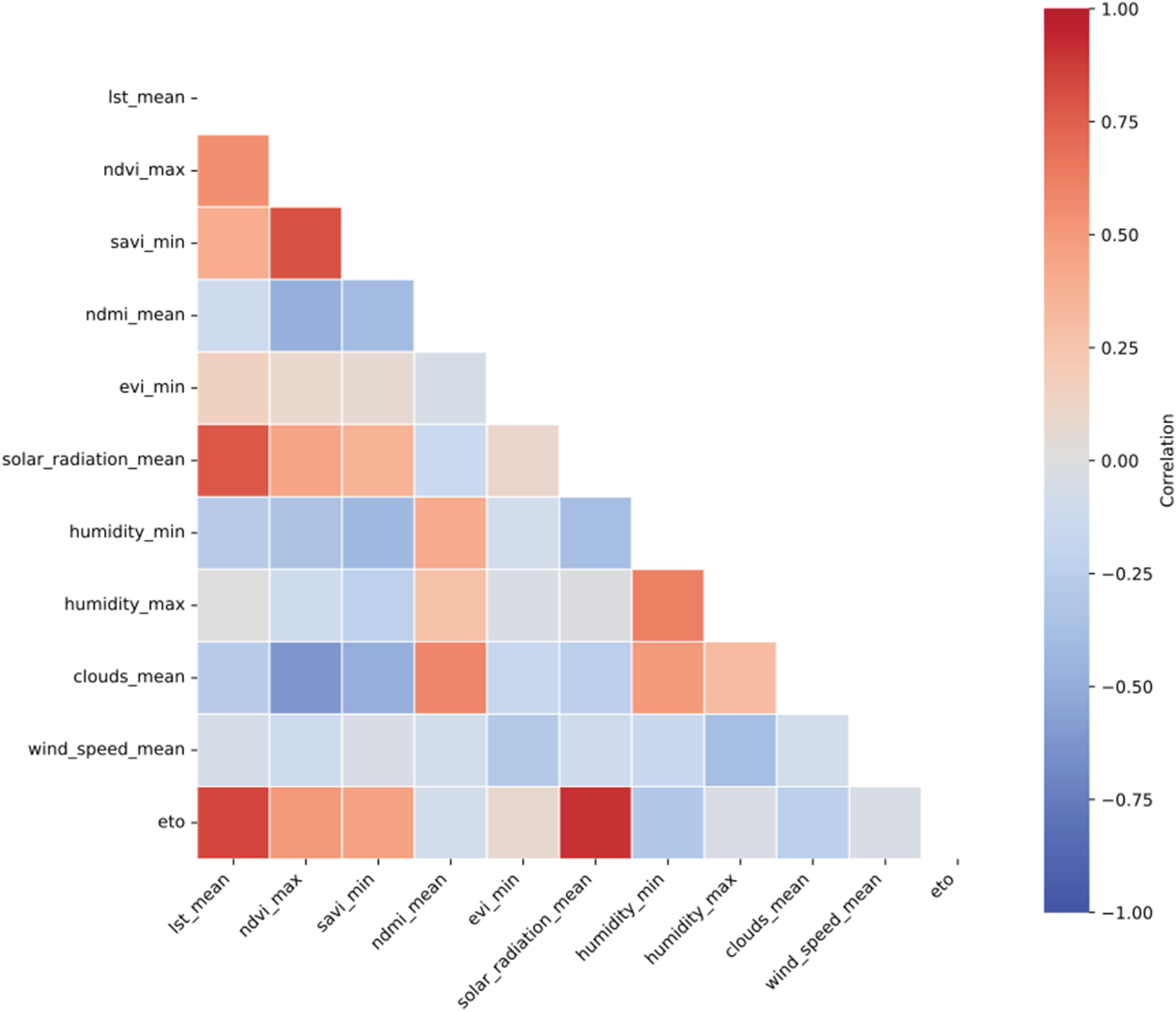
Correlation matrix after multicollinearity reduction.
The resulting dataset retained key indicators:
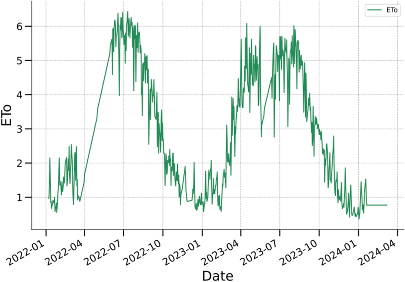
ET0 time series from January 2022 to March 2024 showing the seasonal cycle and interannual variability.
To improve the interpretability of the signal, a three-step preprocessing procedure was applied. First, abrupt and unrealistic changes exceeding 50% relative to the preceding day were flagged as outliers and removed, as these values were inconsistent with the expected seasonal evolution and likely originated from measurement artefacts. Missing values resulting from this filtering were then linearly interpolated to ensure temporal continuity while avoiding bias in subsequent modelling. Finally, a 7-day moving average was applied to smooth high-frequency noise, attenuating short-term variability while preserving the underlying seasonal cycle.
The effect of this procedure is shown in Figure 7, which compares the raw and pre-processed series. The smoothed curve highlights the principal seasonal dynamics and enables a clearer visualization of anomalous periods, such as extreme heat events, without the distraction of erratic day-to-day fluctuations. This preprocessing step thus provides a cleaner and more robust representation of ET0, improving its suitability for downstream modelling and climatological interpretation.
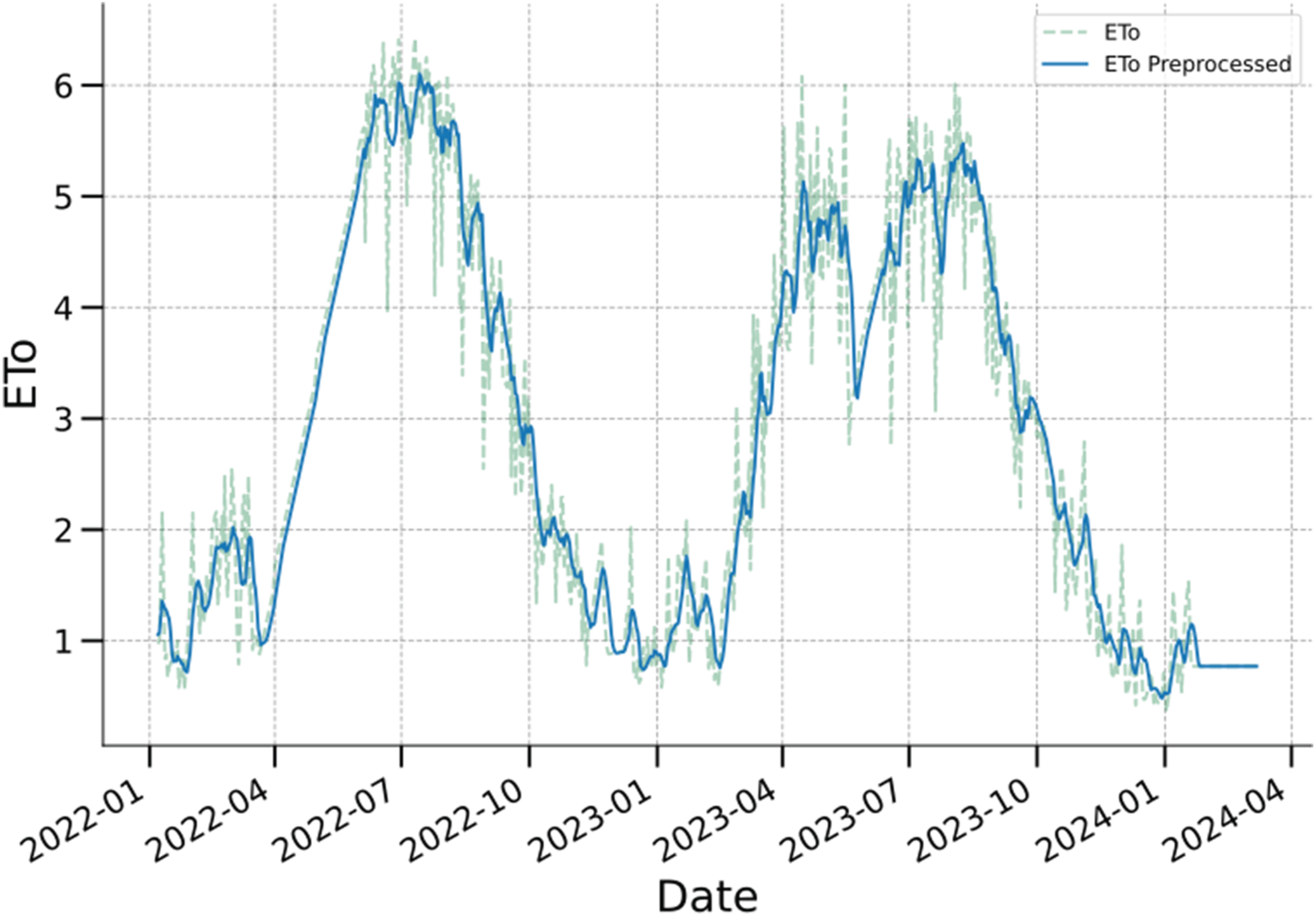
Comparison of raw ET0 data (dashed line) and pre-processed series after outlier removal, interpolation, and 7-day smoothing (solid line).
Machine and DL models
To evaluate the predictive capacity of data-driven approaches for ET0 estimation, a set of ML and DL models were implemented and compared. Classical ML models were used as a performance baseline, while DL architectures were explored for their ability to capture non-linear relationships and temporal dependencies in input variables (Goodfellow et al., 2016; Hastie et al., 2009). This comparative approach enables a comprehensive assessment of model complexity versus predictive performance.
Four classical ML algorithms were selected to provide interpretable baselines and to benchmark the added value of more complex architectures.
where Y denotes ET0, 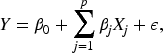
Metrics
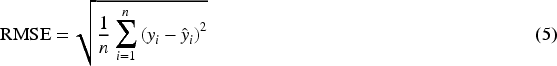
To comprehensively evaluate model performance, four complementary metrics were used (Hastie et al., 2009; James et al., 2013). These metrics capture different aspects of predictive accuracy and allow a robust comparison between models.
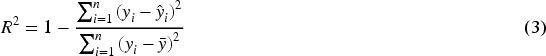
Although widely used, a high R2 value does not guarantee that the model has captured the true underlying relationship, especially for non-linear models. It should be interpreted alongside other metrics to assess a model's ability to generalize to new data.
• 
• 
• 
-------------------------------------------------------------------------------------------------------
The combined use of R2, MSE, RMSE, and MAE provides a balanced assessment of model performance: R2 evaluates overall explanatory power, MSE and RMSE highlight large deviations, and MAE delivers an intuitive measure of typical predictive error.
Experimental design
A series of experiments were conducted to systematically assess the performance of the ML and DL models in predicting ET0. The evaluation relied on the metrics described in Section Metrics, ensuring a comprehensive assessment of predictive accuracy. To obtain robust and unbiased performance estimates, all experiments were carried out using 10-fold cross-validation, which mitigates the risk of overfitting and accounts for data variability.
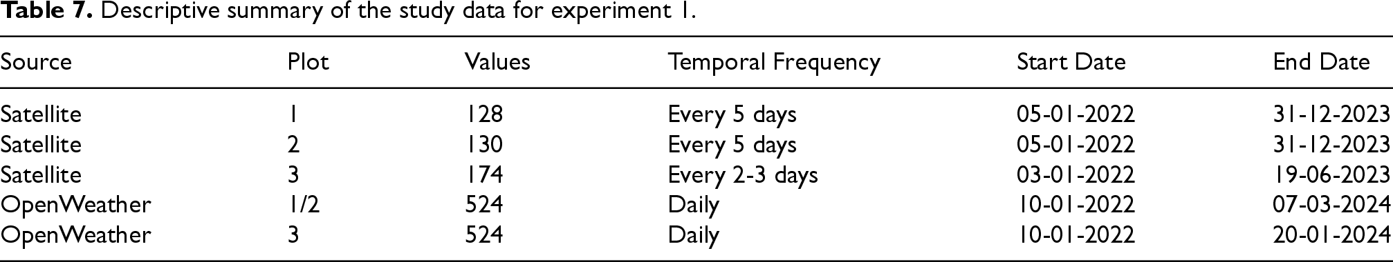
The experimental protocol was structured in three sequential stages. First,
Descriptive summary of the study data for experiment 1.
Three baseline DL architectures were implemented to model the relationship between inputs variables and ET0; a MLP, a 1D-CNN, and a SimpleRNN.
The
The
The
OLS regression was employed to quantify variable importance and assess model diagnostics under each scenario. The initial model (Scenario 1) achieved an R2 of 0.80 but exhibited severe multicollinearity and autocorrelation. Removing non-significant variables (Scenario 2) slightly reduced R2 to 0.78, while worsening multicollinearity due to the disproportionate influence of a smaller set of correlated predictors. The final approach (Scenario 3), which included multicollinearity elimination, yielded a robust yet slightly lower R2 of 0.77 and markedly improved numerical stability, as evidenced by a reduced condition number of 918. This trade-off was considered acceptable as it produced a more reliable model for downstream prediction tasks. The consolidated dataset used in this experiment is summarized in Table 8, while the neural network architectures remained identical to those implemented in the first experiment.
Descriptive summary of the consolidated satellite dataset used in experiment 2.

Three CNN variants and one extended RNN model were evaluated. The baseline
For recurrent modelling, an
This optimization phase enabled a systematic exploration of how network depth, feature extraction capacity, and regularization strategies influence ET0 prediction performance, ultimately identifying architectures that best balance model expressiveness and generalization capability.
Model interpretability: SHAP analysis
To address the need for model transparency and identify the primary drivers of ET0 estimation, an interpretability analysis was performed using SHAP. While DL models like RNNs and CNNs often operate as ‘black boxes’, SHAP values provide a mathematically consistent way to attribute the contribution of each input feature to the final prediction. This analysis was conducted using XGBoost as a surrogate model due to its high performance in complex predictive tasks (Chen and Guestrin, 2016), its proven efficiency in meteorological applications, and its computational compatibility with the SHAP framework (specifically through TreeSHAP) (Lundberg and Lee, 2017). This step ensures that the model's predictive logic aligns with established thermodynamic and aerodynamic principles of evapotranspiration.
Results and discussion
First experiment: Plot-specific modelling and outlier impact
The first experimental stage aimed to establish a performance baseline by training and evaluating models on plot-specific datasets derived from satellite and OpenWeather data. This experiment was conducted in two phases: initially using the raw datasets, and subsequently with outliers removed to quantify their effect on predictive accuracy. As shown in Tables 9 and 10, outlier removal substantially improved model performance across all three plots, leading to higher R2 values and lower MSE. The CNN consistently outperformed other models on the cleaned satellite data, achieving the highest R2 (0.93) and the lowest MSE (0.21) in Plot 2. Both CNN and RNN architectures demonstrated a clear advantage over classical ML models (DT, KNN, LR, RFR), confirming the value of DL for capturing nonlinear relationships and temporal dependencies in ET0 dynamics.
Experiment 1 results for raw satellite data across the three plots.
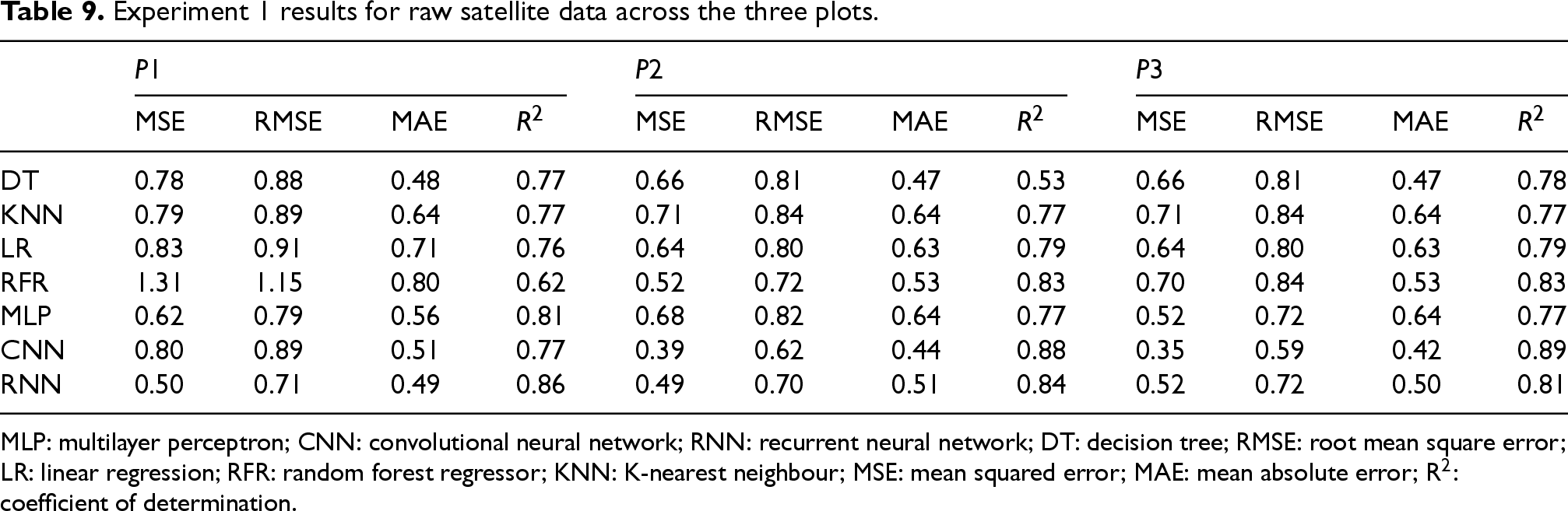
MLP: multilayer perceptron; CNN: convolutional neural network; RNN: recurrent neural network; DT: decision tree; RMSE: root mean square error; LR: linear regression; RFR: random forest regressor; KNN: K-nearest neighbour; MSE: mean squared error; MAE: mean absolute error; R2: coefficient of determination.
Experiment 1 results for satellite data after outlier removal.
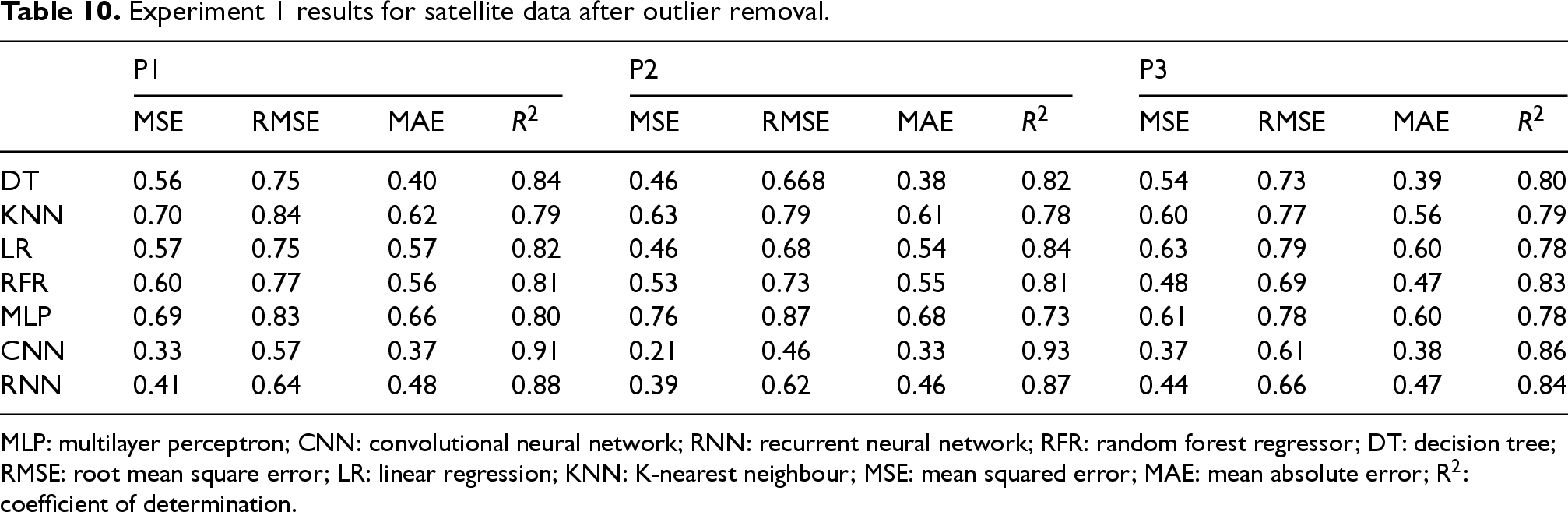
MLP: multilayer perceptron; CNN: convolutional neural network; RNN: recurrent neural network; RFR: random forest regressor; DT: decision tree; RMSE: root mean square error; LR: linear regression; KNN: K-nearest neighbour; MSE: mean squared error; MAE: mean absolute error; R2: coefficient of determination.
When using OpenWeather data, models achieved slightly higher R2 values overall (see Table 11), benefiting from the larger sample size and daily temporal resolution. However, the performance gap relative to satellite-based models was marginal and given the broader accessibility and reproducibility of open satellite data, subsequent experiments focused exclusively on the satellite-derived dataset.
Experiment 1 results for OpenWeather data.
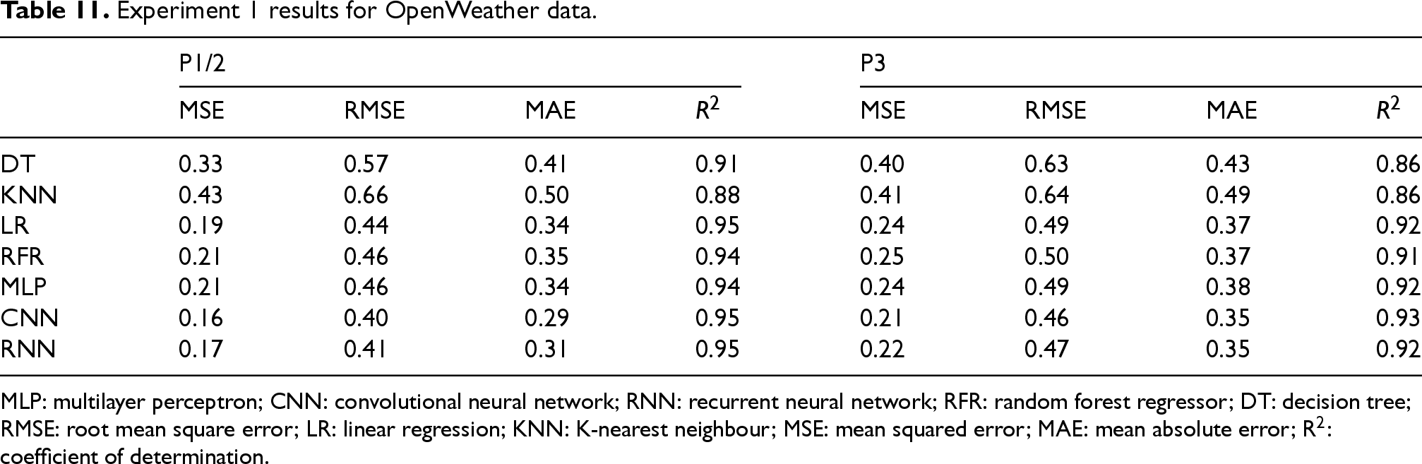
MLP: multilayer perceptron; CNN: convolutional neural network; RNN: recurrent neural network; RFR: random forest regressor; DT: decision tree; RMSE: root mean square error; LR: linear regression; KNN: K-nearest neighbour; MSE: mean squared error; MAE: mean absolute error; R2: coefficient of determination.
Second experiment: Generic modelling with multicollinearity mitigation
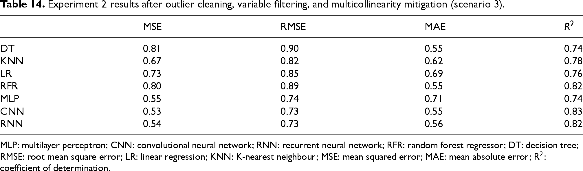
The second experimental stage aimed to construct a generalized modelling framework by pooling satellite data from all plots into a single consolidated dataset. This experiment was designed to evaluate the impact of preprocessing and feature selection on model performance, with the goal of producing a robust model applicable across heterogeneous locations without plot-specific retraining. Three modelling scenarios were compared. In Scenario 1, all available variables were retained following outlier cleaning. Scenario 2 employed statistical filtering by discarding variables with p-values greater than 0.02 as determined by an OLS regression analysis. Scenario 3 extended this approach by also mitigating multicollinearity, removing redundant predictors identified through pairwise Pearson correlations exceeding
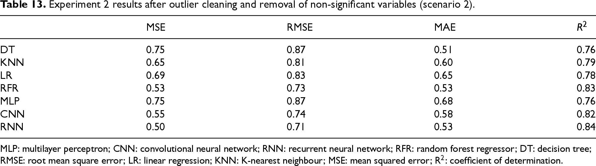
OLS regression was used not only to assess variable significance but also to diagnose model quality, under the assumptions of linearity, independence, homoscedasticity, and normality of residuals. The initial model (Scenario 1) achieved an R2 of 0.80 but suffered from strong multicollinearity and autocorrelation effects, as indicated by an elevated condition number. Removing non-significant variables (Scenario 2) slightly reduced R2 to 0.78 and, paradoxically, exacerbated multicollinearity by increasing the relative influence of correlated predictors. The final scenario (Scenario 3) resulted in a slightly lower R2 of 0.77 but markedly reduced the condition number to 918, indicating improved numerical stability. This trade-off was considered favourable, as the resulting model offered a more interpretable and statistically sound baseline.
Tables 12, 13, and 14 summarize model performance under the three scenarios. In all cases, CNN and RNN architectures consistently outperformed traditional models in terms of R2 and error metrics, highlighting their robustness to correlated features and their capacity to capture nonlinear relationships. Importantly, the reduction of multicollinearity did not degrade DL performance, reinforcing the generalization ability of these architectures.
Experiment 2 results after outlier cleaning (scenario 1).
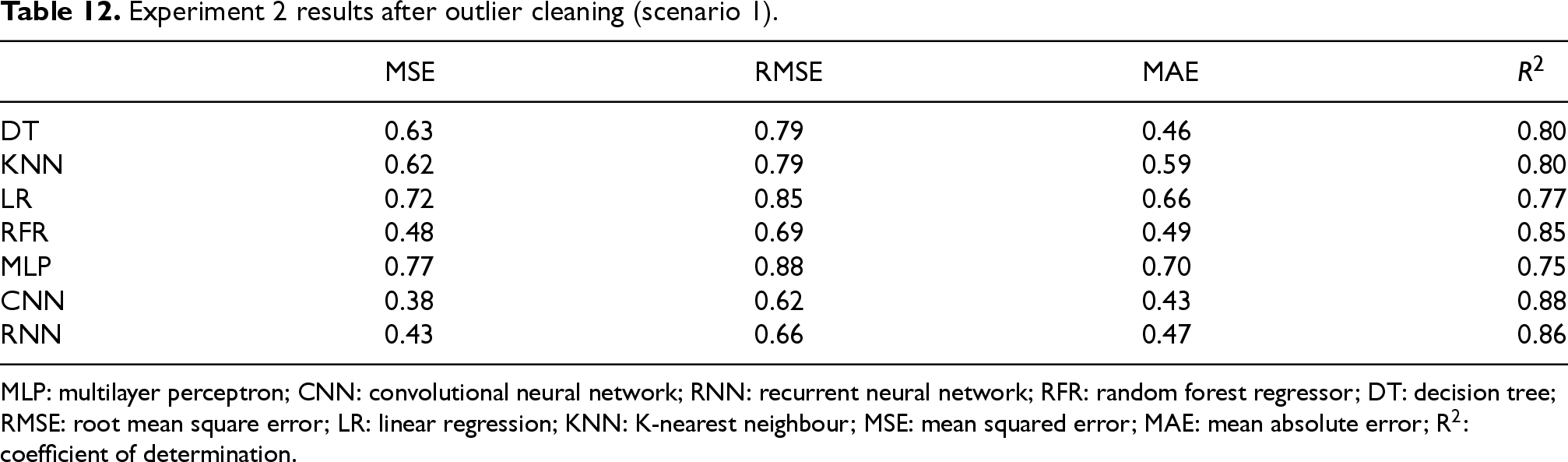
MLP: multilayer perceptron; CNN: convolutional neural network; RNN: recurrent neural network; RFR: random forest regressor; DT: decision tree; RMSE: root mean square error; LR: linear regression; KNN: K-nearest neighbour; MSE: mean squared error; MAE: mean absolute error; R2: coefficient of determination.
Experiment 2 results after outlier cleaning and removal of non-significant variables (scenario 2).
MLP: multilayer perceptron; CNN: convolutional neural network; RNN: recurrent neural network; RFR: random forest regressor; DT: decision tree; RMSE: root mean square error; LR: linear regression; KNN: K-nearest neighbour; MSE: mean squared error; R2: coefficient of determination.
Experiment 2 results after outlier cleaning, variable filtering, and multicollinearity mitigation (scenario 3).
MLP: multilayer perceptron; CNN: convolutional neural network; RNN: recurrent neural network; RFR: random forest regressor; DT: decision tree; RMSE: root mean square error; LR: linear regression; KNN: K-nearest neighbour; MSE: mean squared error; MAE: mean absolute error; R2: coefficient of determination.
Third experiment: Optimization of CNN and RNN architectures
The third experimental stage focused on refining the baseline DL architectures to maximize predictive performance. Specifically, we investigated the effect of architectural modifications, such as increasing network depth, incorporating additional convolutional layers, and applying regularization strategies like dropout-on the ability of CNN and RNN models to capture the temporal dynamics of ET0. All models were trained and evaluated using the consolidated satellite dataset from Experiment 2 to ensure comparability. Table 15 summarizes the results of this optimization study. Among the evaluated models, the optimized RNN achieved the best performance, with an R2 of 0.92, an MSE of 0.23, and an MAE of 0.23. These results confirm the ability of recurrent architectures to effectively model sequential dependencies in agroclimatic data, outperforming both the baseline CNN configurations and the RFR. Notably, CNN_3, which incorporated multiple convolutional layers and dropout regularization, exhibited a marked improvement over the baseline CNN_1, reinforcing the benefit of deeper architectures for feature extraction.
Experiment 3 results after cnn/rnn architecture optimization.
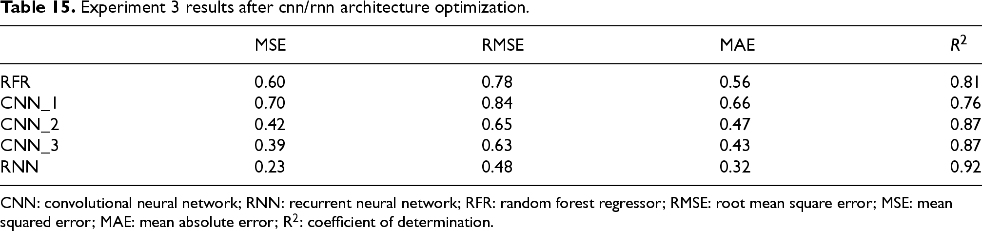
CNN: convolutional neural network; RNN: recurrent neural network; RFR: random forest regressor; RMSE: root mean square error; MSE: mean squared error; MAE: mean absolute error; R2: coefficient of determination.
Figures 8, 9, and 10 show these findings. The parity plot for the RNN (see Figure 8) shows predictions closely aligned with the 1:1 reference line, indicating minimal systematic bias. The histogram of residuals (see Figure 9) displays a sharp concentration of errors around zero, highlighting the model's high overall accuracy. Finally, the time series example from a cross-validation fold (see Figure 10) demonstrates that the RNN effectively captures intra-seasonal patterns and peak evapotranspiration events, though slight under- and over-predictions remain visible at extreme values, suggesting potential areas for further refinement.
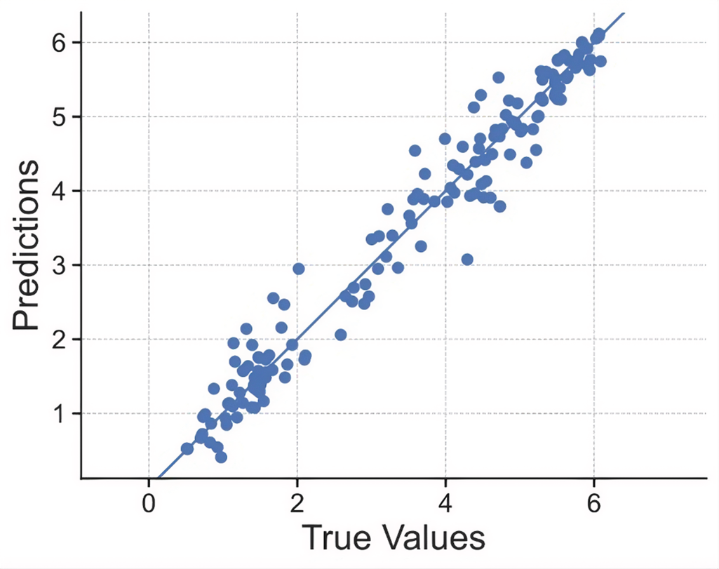
Parity plot comparing predicted and observed ET0 values for the optimized recurrent neural network (RNN).
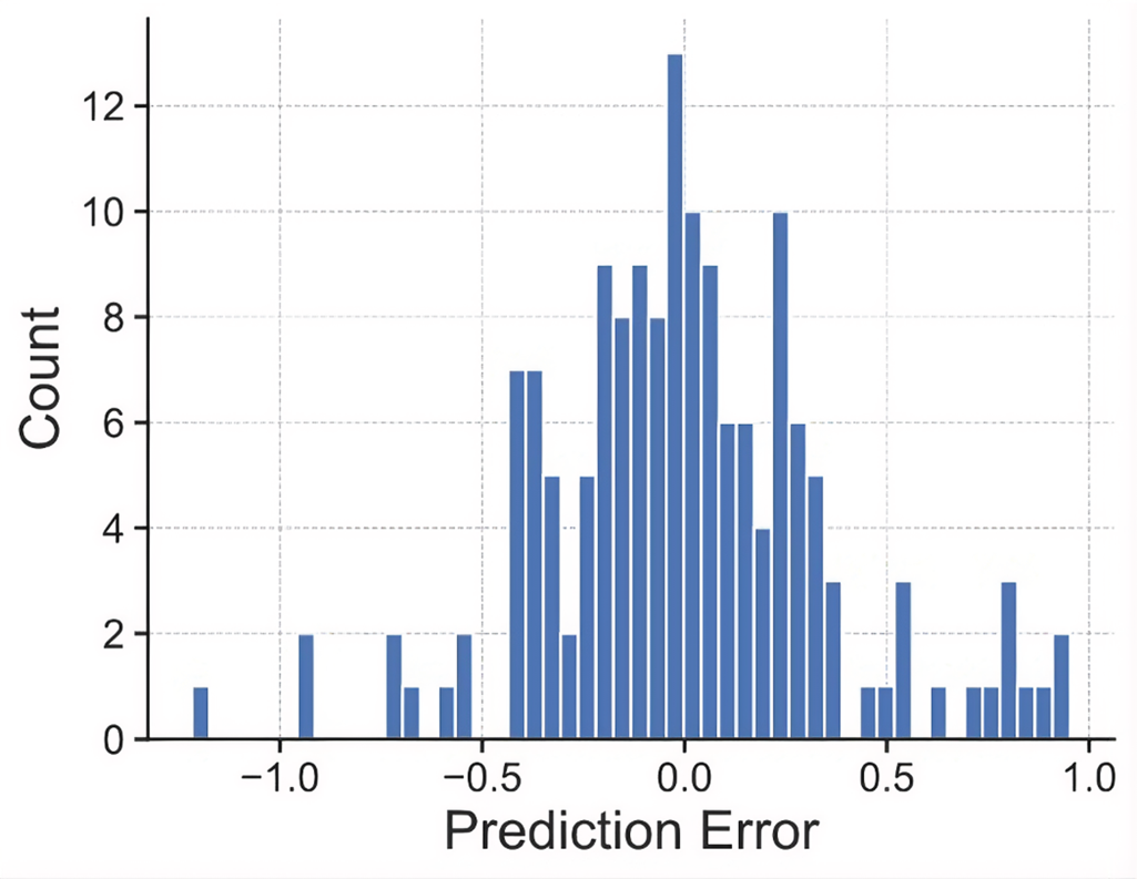
Histogram of residuals for the optimized recurrent neural network (RNN) model, showing error distribution concentrated near zero.
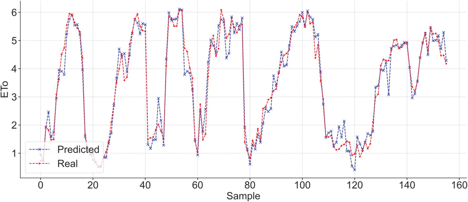
Example of predicted versus observed ET0 values in one cross-validation iteration.
These results confirm that optimizing DL architectures, particularly through deeper recurrent networks, yields substantial gains in predictive accuracy. The strong performance of the RNN highlights its potential as a core modelling approach for sequential agroclimatic prediction tasks and for supporting operational decision-making in precision irrigation management.
Interpretability analysis and biophysical consistency
The exceptional predictive performance of the RNN model (R2 = 0.92) is rooted in its ability to internalize complex land-atmosphere interactions. To validate this, a SHAP analysis was conducted to bridge the gap between the network's ‘black box’ nature and the underlying physical processes. As illustrated in Figure 11, the model exhibits a clear hierarchical structure dominated by LST (lst\_mean). Acting as the primary forcing variable, LST yields a mean absolute SHAP value of 1.33, significantly outweighing secondary spectral predictors.
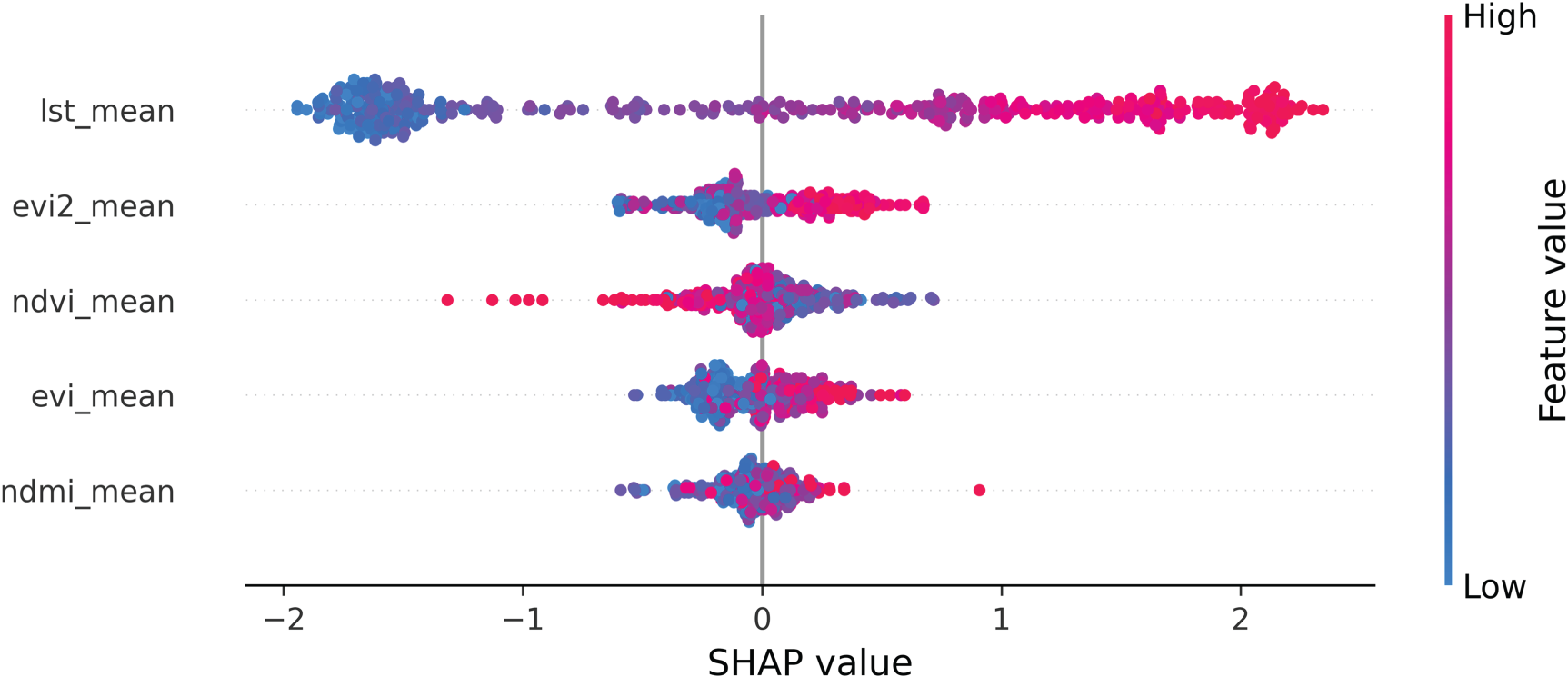
SHAP interpretation of the RNN model. (a) Global feature importance highlighting the dominance of lst\_mean. (b) Summary plot showing the directional impact of biophysical predictors. The R2 = 0.92 is supported by the strong alignment of thermal (LST) and vegetation (EVI2/NDVI) drivers with established ecosystem dynamics. RNN: recurrent neural network; SHAP: SHapley Additive exPlanations; NDVI: normalized difference vegetation index; EVI: enhanced vegetation index; LST: land surface temperature.
The SHAP summary plot reveals a robust biophysical alignment that justifies the model's high accuracy. The positive correlation between elevated LST values (red points) and increased model output confirms that the RNN correctly identifies thermal energy as the primary driver. Interestingly, the model captures divergent behaviours among vegetation indices: while evi2\_mean and evi\_mean contribute positively, high values of ndvi\_mean exert a negative pressure on the output. This indicates that the RNN is not merely over-fitting spectral greenness; rather, it is likely accounting for the ‘saturation effect’ of NDVI or the evaporative cooling feedback loops typically associated with dense canopy covers.
Furthermore, the inclusion of the moisture index (ndmi\_mean) provides a critical baseline for water availability, allowing the model to distinguish between energy-limited and water-limited regimes. The convergence of these factors-thermal forcing, structural vegetation dynamics, and moisture constraints-within the RNN's temporal learning framework explains its superior generalization capability. These findings demonstrate that the 0.92 accuracy is not a product of stochastic correlation, but a reflection of the model's capacity to mirror the non-linear physical principles governing the ecosystem.
Discussion
This study provides robust evidence supporting the use of DL methodologies for ET0 estimation based solely on open-access data. Our results demonstrate that RNNs deliver superior predictive performance, achieving a coefficient of determination of R2 = 0.92, outperforming CNNs, MLPs, and classical ML models. The advantage of RNNs can be attributed to their architectural capacity to model temporal dependencies, enabling them to capture lagged interactions and cumulative effects of climatic variables that drive evapotranspiration processes. Preserving temporal context is crucial for accurately characterizing intra- and inter-seasonal dynamics. This result also aligns with findings reported in previous studies on sequential environmental modelling.
The high predictive accuracy (R2 = 0.92) is underpinned by the model's biophysical consistency. By prioritizing LST as the primary forcing variable, the RNN aligns with energy-balance principles, where thermal dynamics drive the modelled processes. Furthermore, the divergent response between NDVI and EVI2 in the SHAP analysis is scientifically significant; it indicates that the RNN has learned to mitigate the saturation effects typical of NDVI in dense vegetation. By counter-balancing these indices, the architecture achieves a more robust generalization, proving that the high performance is a result of capturing complex land-surface interactions rather than simple numerical overfitting.
The superior performance of RNNs over CNNs can be explained by the temporal nature of ET0 dynamics. Evapotranspiration is strongly influenced by multi-day accumulations of radiation, humidity, and soil moisture. While 1D-CNNs capture local temporal windows, they lack the long-range memory preserved by RNNs. This explains why RNNs consistently yielded higher accuracy in sequential agroclimatic prediction tasks.
An important methodological contribution of this work lies in the systematic treatment of input features. Through OLS regression analysis and correlation-based feature reduction, we eliminated non-significant and highly collinear predictors, improving model interpretability and computational efficiency while maintaining predictive accuracy. This stepwise feature selection strategy not only reduced redundancy but also mitigated numerical instabilities, as indicated by the reduced condition number in Experiment 2. These improvements were particularly relevant for linear models but also provided cleaner, better-conditioned inputs for DL architectures, thereby enhancing their generalization ability. While recent advances in DL have introduced hybrid models and metaheuristic-optimized frameworks (such as RNN long short-term memory (LSTM) or ANN-GWO) that achieve high precision, these typically depend on high-quality data from local physical meteorological stations. Our study diverges from this trend by focusing on an ‘infrastructure-free’ paradigm. We explore how DL architectures can compensate for the lack of in-situ sensors by effectively fusing heterogeneous, open-access data from satellite imagery and global climate services.
However, despite these advances, there is still a gap in infrastructure-free models. Therefore, the main contribution of this research is the demonstration of an infrastructure-independent, reproducible approach for ET0 estimation. By leveraging exclusively RS products and publicly available climate service data, our models match or exceed the accuracy of approaches relying on traditional meteorological station networks, and in some cases surpass hybrid models that combine ground-based and RS inputs. This finding is of particular significance for regions with limited meteorological infrastructure, where station installation and maintenance are logistically and financially challenging. The proposed framework thus offers a scalable, cost-effective solution for operational water resource management.
Beyond methodological advances, the implications for agricultural practice are considerable. Accurate and spatially explicit ET0 predictions enable improved irrigation scheduling, promote efficient water allocation, and contribute to sustainable agricultural production under increasing climate variability. In this context, our results support the integration of DL models, particularly RNN-based architectures, into digital agriculture platforms and decision-support systems, fostering data-driven strategies for enhancing water-use efficiency and climate resilience in irrigated systems.
It is worth noting that classical models such as LR and RFR remain valuable in contexts with limited datasets, where training speed, computational simplicity, or interpretability are priorities. In operational settings with scarce data or resource constraints, these models can still provide actionable insights, albeit with lower accuracy than DL approaches.
While simpler architectures such as the M5 Tree have shown competitive performance in specific case studies due to their transparent structure and lower computational requirements (Dadrasajirlou et al., 2022), they may lack the capacity to fully capture the complex, non-linear, and multi-dimensional spatial-temporal relationships inherent in satellite-derived data. Our findings suggest that, for an infrastructure-free framework relying on RS, the superior feature extraction capabilities of DL architectures (RNNs and CNNs) provide a necessary advantage over these simpler tree-based models.
Conclusions and future work
This research clarifies the trade-off between model complexity and data accessibility. We have shown that the inherent ability of RNNs to handle long-term dependencies in climatic time series allows for an ET0 estimation that is independent of local infrastructure, representing a significant shift from traditional hybrid models that are constrained to sensor-dense environments.
Building on this premise, our study establishes a robust and reproducible DL framework for estimating ET0 exclusively from open-access RS and climate service data. Among the evaluated approaches, RNNs consistently yielded the best performance, achieving an R2 of 0.92, confirming their ability to capture the temporal dependencies inherent in agroclimatic time series.
This high predictive accuracy is further supported by SHAP interpretability analysis, which confirms that the model's internal logic is strictly aligned with biophysical principles. By identifying LST (lst\_mean) as the primary driving force and effectively integrating vegetation and moisture dynamics, the RNN demonstrates a physically consistent behaviour. This ensures that the model is not merely a ‘black-box’ numerical fit but a robust representation of the energy-balance processes governing evapotranspiration.
Importantly, this level of accuracy was obtained without reliance on conventional ground-based meteorological stations, validating the feasibility of an infrastructure-independent approach to ET0 modelling. A key methodological contribution of this study lies in the rigorous feature selection process based on OLS regression and multicollinearity reduction. This procedure not only improved model interpretability and computational efficiency but also ensured numerical stability, providing a robust baseline for evaluating more complex models. Collectively, these contributions advance the state of the art by delivering a scalable, cost-effective solution for water resource monitoring that is particularly relevant for regions with limited or absent meteorological infrastructure. The broader implications of this work are significant. The proposed methodology:
Facilitates more informed irrigation scheduling, Improves water-use efficiency, and Supports sustainable agricultural production in the face of increasing climate variability.
By leveraging open data, the approach democratizes access to advanced decision-support tools, enabling equitable and data-driven water management at regional and global scales.
Building upon these findings, future research will pursue several avenues. First, we plan to expand the dataset to include additional agroecological zones, climatic regimes, and crop types worldwide, thereby enhancing model generalizability and enabling robust performance across diverse production systems. Second, we will investigate the integration of additional explanatory variables, such as high-resolution soil moisture measurements, soil physical and chemical characteristics, and crop-specific coefficients, to extend the modelling framework from ET0 to actual crop evapotranspiration (ETC). Finally, we will explore more advanced neural architectures, including LSTM networks and Transformer-based models, to further improve the capacity for capturing long-range dependencies and enhancing forecasting accuracy. The ultimate objective is to transition from ET0 estimation to predictive modelling capable of supporting proactive irrigation management and adaptive strategies for climate-resilient agriculture.
Overall, the proposed framework represents a step toward the democratization of PA. By eliminating the dependency on costly in situ maintenance, this model provides a scalable tool for sustainable water management in regions where meteorological data scarcity previously hindered the adoption of advanced irrigation strategies.
Footnotes
ORCID iDs
Funding
The authors disclosed receipt of the following financial support for the research, authorship, and/or publication of this article: This work was partially funded by the R&D project MORELLINO (CIPROM/2023/29) through the ‘Direcció General de Ciència i Investigació’ (Generalitat Valenciana, Spain); by the European Union NextGenerationEU/PRTR and project AM-DS (INREED/2024/1) under the Recovery, Transformation and Resilience Plan (GVANEXT, Generalitat Valenciana); and by the European Union under the European Regional Development Fund (ERDF) Programme Comunitat Valenciana 2021–2027, through the IVACE + i Innovation calls for ‘Strategic Cooperation Projects’ (Ref. INNEST/2025/486). This research is also part of the R&D project CPP2021-008722, funded by MCIN/AEI (10.13039/501100011033) and the European Union through NextGenerationEU/PRTR. Additionally, it was supported by the Universitat Politècnica de València (UPV) through the Predoctoral Research Programme (Subprogramme 1, Grant PAID-01–24) funded by the Vice-Rectorate for Research.
Declaration of conflicting interests
The authors declared no potential conflicts of interest with respect to the research, authorship, and/or publication of this article.