A finite element analysis engineering solution to short riveted connections under dynamic loadings

Abstract

The research presented in this manuscript focuses on the development of an LS-DYNA finite element model to predict the dynamic shear strength of short riveted lap-spliced specimens. Using data collected from experimental testing at the U.S. Army Engineer Research and Development Center (ERDC), a finite element model was developed to replicate the behavior of A502 Grade short riveted connections under quasi-static loading. Subsequent analyses used published Cowper-Symonds constitutive model coefficients to replicate the behavior of these connections under dynamic loading. Computed results were then compared with available test data from ERDC. Given the challenges involved in creating physical models with riveted connections and the abundance of historical bridges constructed with rivets, the developed finite element analysis engineering solution can serve as a critical tool for researchers interested in predicting the response of short riveted connections to dynamic loading and those interested in developing strategies to mitigate against this loading.

Keywords

Rivets dynamic loading quasi-static loading shear strength Cowper-Symonds dynamic increase factor

Introduction

Most historical suspension bridges consist of tall steel towers that support the majority of the bridge’s gravity load, including the attached cables, bridge deck, and traffic. While the preferred steel fastener today is the high-strength bolt, historical bridges such as the Golden Gate Bridge and Manhattan Bridge, built prior to1950, were constructed with hot-driven rivets. These iconic bridges are not only considered masterful pieces of “critical infrastructure,” they may also be targets for terrorist organizations. A Blue Ribbon Panel of bridge and tunnel experts from academia, government agencies, and professional practice predicted the replacement cost for one of these iconic bridges is approximately $10 billion (FHWA, 2003). There is no doubt that an attack on an iconic bridge would have significant economic, psychological, and potentially deadly toll on a large population. Despite nearly two decades of the Global War on Terror, statistics obtained from the National Consortium for the Study of Terrorism and Responses to Terrorism (START), shown in Figure 1, demonstrate the likelihood of a terrorist attack today remains at a historical high level (National Consortium for the Study of Terrorism and Responses to Terrorism, 2018).

Figure 1.

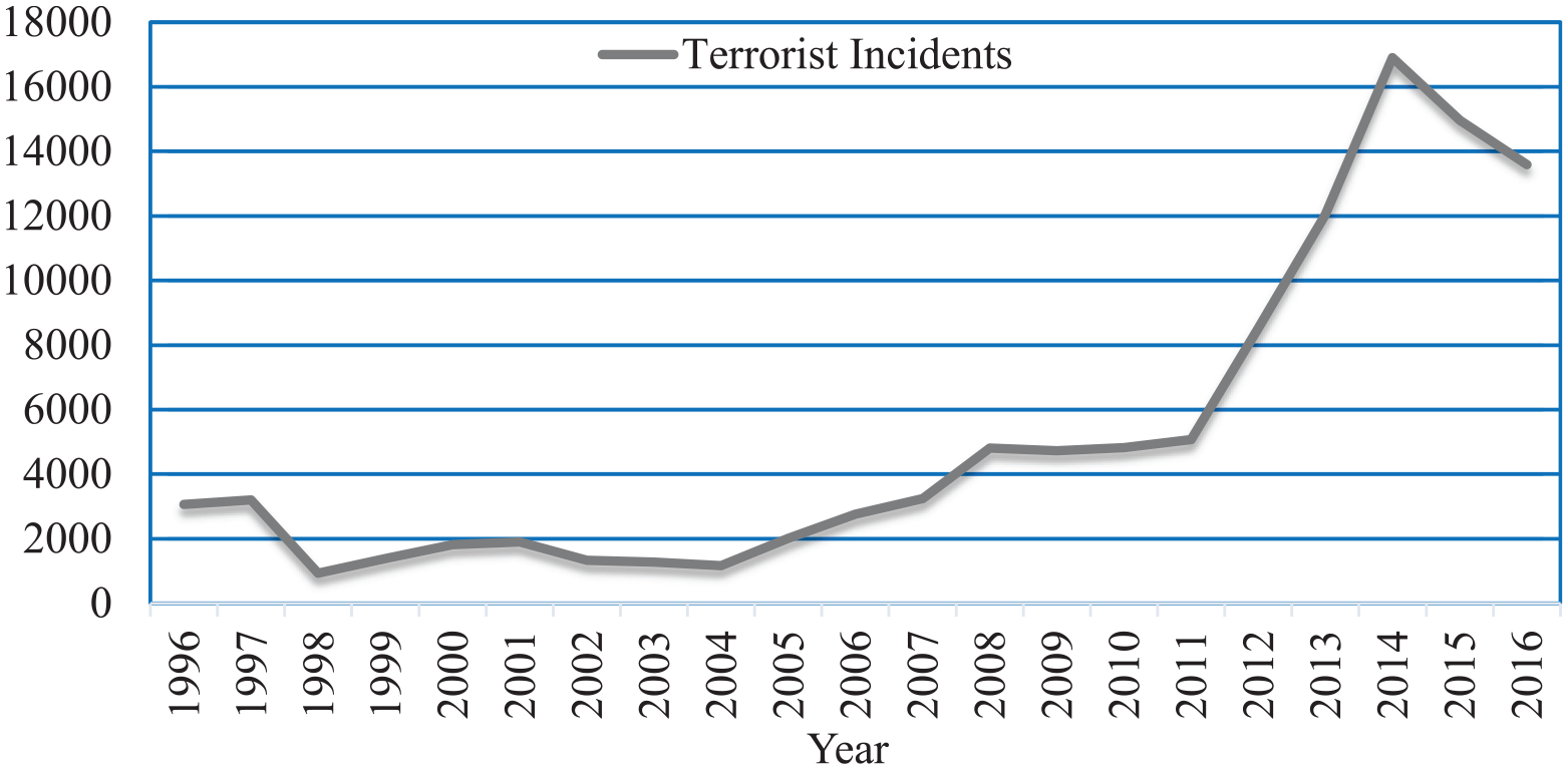
Terrorists incidents over last 20 years (data from National Consortium for the Study of Terrorism and Responses to Terrorism, 2018).

While many engineers are familiar with the behavior and ultimate strength of A325 and A490 bolts, there is little familiarity with the strength of steel rivets. Most research literature regarding the behavior of rivets and riveted connections was published between 1930 and 1970. The stress strain curves for both bolts and rivets are shown in Figure 2. According to the Guide to Design Criteria for Bolted and Riveted Joints, the tensile strength for A502 rivets ranges from 60 ksi for Grade 1 to 80 ksi for Grade 2 and Grade 3 (Kulak et al., 1987). Despite both the aforementioned Manhattan and Golden Gate Bridges already being fully constructed, the first AISC standard to address joints and their fasteners was not published until 1947, with the formation of the Research Council on Riveted and Bolted Structural Connections (currently known as the Research Council on Structural Connections).

Figure 2.

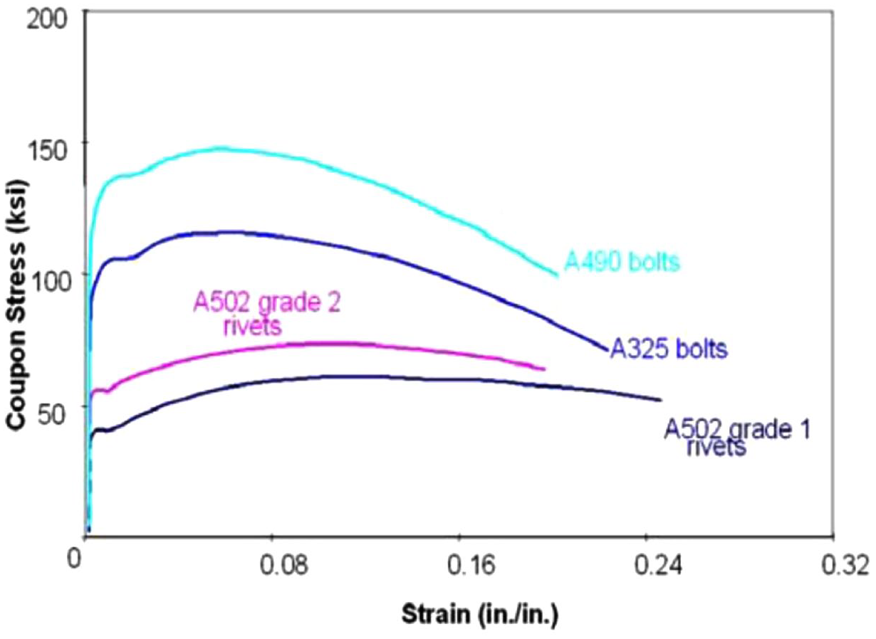
Coupon stress versus strain relationship for rivet and bolt materials (Kulak et al., 1987).

A consistent take-away from the literature lies in the variability of the tensile strength of riveted connections. Pure tension studies conducted at the University of Illinois and the University of Toronto concluded that rivet strength varied based on type of head, length of grip, and whether it was driven by a pneumatic hand riveting hammer or a hydraulic riveting machine, just to name a few (Wilson and Oliver, 1930; Wilson and Thomas, 1938; Young and Dunbar, 1928). The research literature also shows there is a direct correlation between the shear strength and tensile strength of riveted connections (Munse and Cox, 1956). The Guide to Design Criteria for Bolted and Riveted Connections reports an average shear-to-tensile strength ratio varying from 0.67 to 0.83, with an average of 0.75 (Kulak et al., 1987). Testing variables such as rivet size, grip, method of driving, and the method of rivet manufacturing all contributed to the range, while having little effect on the average value. Thus, for current ASTM A502 Grade 1 and Grade 2 rivets with tensile strengths of 60 and 80 ksi respectively, expected shear strengths are between 45 ksi and 60 ksi for Grade 1 rivets and between 60 ksi and 80 ksi for Grade 2 rivets. Until recently, literature has focused on quasi-static rivet strength in tension, shear, and combinations of tension and shear.

The behavior of structures to dynamic loads such as blast differs in comparison to quasi-static loads. Loadings over a very short duration must account for time-dependent behavior. Thus, the analysis must consider dynamic structural response and consideration of inertial effects. Further, for blast loads, inelastic material response under high strain rates must also be considered. Under dynamic loading, steel materials achieve an enhanced strength that boosts its ability to resist loads. As the material is loaded rapidly, it cannot deform at the same rate at which the load is applied. Thus, a greater load is required to produce the same deformation than at a lower strain rate. For most steels, the modulus of elasticity and ultimate strain of steel are largely unaffected; however, a high strain rate creates an increase in the stress level at which both the yield stress (up to 35%) and the ultimate stress occurs (up to 10%). These large increases are too significant to be ignored when predicting response. The increase in strength associated with the rapidly applied load is known as the dynamic increase factor (DIF) and is expressed numerically as the ratio of dynamic-to-static stress.

Objectives

The Mineta Transportation Institute released a report in 2016 discussing long-term trends in attacks on public surface transportation and revealed that 65% of attacks worldwide were bombings (Jenkins, 2016). With historical bridges such as the five-mile Mackinac Bridge in Michigan being held together with millions of rivets (4,851,700 steel rivets for the Mackinac Bridge) (Steinman and Nevill, 1957), an understanding of their behavior, and that of other historical riveted bridges, under high loading rates is critical. Thus, the purpose of the research presented in this manuscript is to develop a finite element analysis (FEA) engineering solution for predicting the response of short riveted connections subjected to high-intensity, short-duration dynamic loading. Such information is needed to develop strategies for mitigating blast loads.

This research has two primary objectives:

Provide direction on modeling rivets using the nonlinear transient dynamic FEA software package LS-DYNA.

Provide direction on modeling strain rate effects for short riveted connections using LS-DYNA.

Quasi-static finite element model

Little if any research investigating the response of riveted connections to blast loads had been performed until laboratory and field tests were completed by the ERDC, USACE. In research performed for the U.S. Department of Homeland Security and the Federal Highway Administration, ERDC conducted comparative explosion tests on bridge tower components. Initial tests included an investigation of scaled models of steel bridge tower components using mild steel (Walker et al., 2011a, 2011b, 2011c, 2011d). The results of this testing showed the riveted panels demonstrated a ductile, tension failure, with a 35% reduction in steel plate cross-sectional area at the failure site (Crane et al., 2015). Meanwhile, the ASTM A502 standard strength rivets exhibited absolutely no reduction in cross-sectional area, thus exhibiting a pure shear failure.

Following this pure shear failure response, ERDC conducted short-duration, monotonic dynamic loads on 86 riveted lap-spliced specimens using a 200-kip dynamic loader (Rabalais, 2015). Testing included an investigation into the shear failure of four distinct variables of short riveted connections (fastener type, single shear or double shear, joint configuration type and loading type) over a period within 1 to 6 milliseconds (msec). The authors found A502 rivets to have a 1.72 dynamic increase factor for the quasi-static shear strength.

Based on the field and laboratory testing by ERDC, the authors of this paper started developing their LS-DYNA model by focusing on the finite element analyses of rivets under quasi-static loading conditions. Critical aspects of this modeling include discretization, approximation of boundary conditions and loading, and determination of a material model to dictate behavior. LS-DYNA simulates the response of the defined model by conducting a highly nonlinear, transient dynamic finite element analysis using explicit time integration. The analysis is nonlinear in that the rivet experiences severe deformations prior to rupture, the rivet material properties exhibit nonlinear response, and the contact between parts (the rivet(s) and the plates) changes over time.

Solid elements were used to develop the FEA models presented in this paper. The advantages to solid elements are that they are three-dimensional finite elements that can model solid bodies and structures without geometric simplifications; thus, the assembled finite element mesh is nearly identical to the physical system. The only differences between the physical test specimen and the FEA model are due to slight approximations in geometry that are a function of the element type and mesh discretization selected. Using linear elements for a curved geometry lend itself to modeling errors in FEA (Melosh, 1993). Eight-node hexahedra elements were used for the model as they are easier to visualize, more computationally efficient, and have proven to provide more accurate results when compared to tetrahedron elements (Erhart, 2011). Perhaps more importantly, tetrahedron elements behave poorly in cases where elements are loaded in shear, while hexahedron elements with adequate discretization refinement approximate analytical solutions (Erhart, 2011).

After choosing the element type (8-node hexahedra elements), the element formulation also needed to be selected. Different formulations affect solution accuracy. Stresses and strains are calculated at each integration point, and displacements are calculated at each node. Options considered for this research within LS-DYNA included ELFORM 3 (fully integrated solid elements), ELFORM 2 (partially integrated solid elements), and ELFORM 1 (under-integrated constant stress elements). Under-integrated elements describe an element formulation in which stresses and strains are only calculated at the mid-point of each element. The full integration and reduced integration options are typically two to four times costlier than the under-integrated element formulation, because they calculate the stiffness and mass at several more sampling (or integration) points within an element. The under-integrated element formulation has also been shown to be more accurate in situations with significant deformations (LS-DYNA Theory Manual, 2006). Thus, while the accuracy of integration is increased with additional integration points, the finite elements results are not necessarily improved.

Despite the potential for improved performance, one of the issues with the under-integrated element formulation is the possibility of spurious deformation modes of the finite element mesh. An example of this phenomenon is shown in Figure 3. In a situation where this element is subjected to pure bending, neither of the element characteristic lengths (a to b and c to d) change in length. The under-integrated stiffness matrix for this element only contains information at the center of the element (in this example, where the two dashed lines meet). The result is a zero-energy mode where all the components of stress at the single integration point are zero. The element has no stiffness in this mode and is unable to resist this type of deformation. An accumulation of this energy mode throughout a mesh will give inaccurate results. This type of energy mode is known as “hourglassing” energy because the deformed shape resembles an hourglass.

Figure 3.

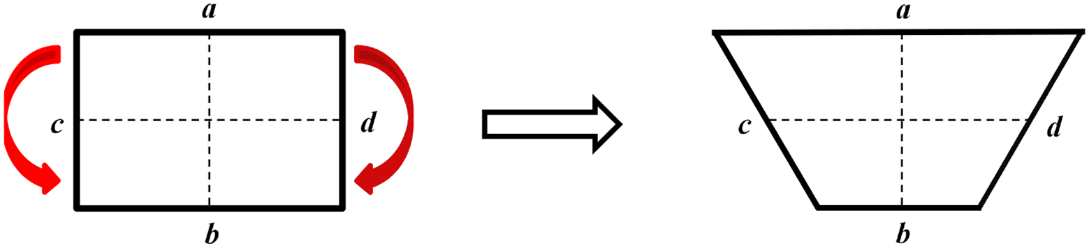
Spurious deformation for under-integrated element.

LS-DYNA provides the user with a warning of spurious deformations by providing the histories of the hourglass energy. As a general rule, the hourglass energy should be less than 5%–10% of the internal energy (LS-DYNA Theory Manual, 2006). Physically, hourglass issues are evident by the zig-zag appearance of element shapes. LS-DYNA offers 12 different hourglass modes to help control spurious deformations for solid elements. These algorithms provide forces, or hourglass energy, to resist hourglass modes. A simple example where internal nodal forces are introduced to counteract the hourglass mode issue demonstrated in Figure 4. The viscous forms of hourglass control (HG1, HG2, and HG3) are designed for analyses involving high strain rates because the algorithm generates hourglass forces proportional to the components of nodal velocity contributing to the hourglass modes (Forsberg, 2013). The stiffness forms of hourglass control (HG4 and HG5) are typically preferred for slower strain rate problems; they generate hourglass forces proportional the components of nodal displacement (Forsberg, 2013).

Figure 4.

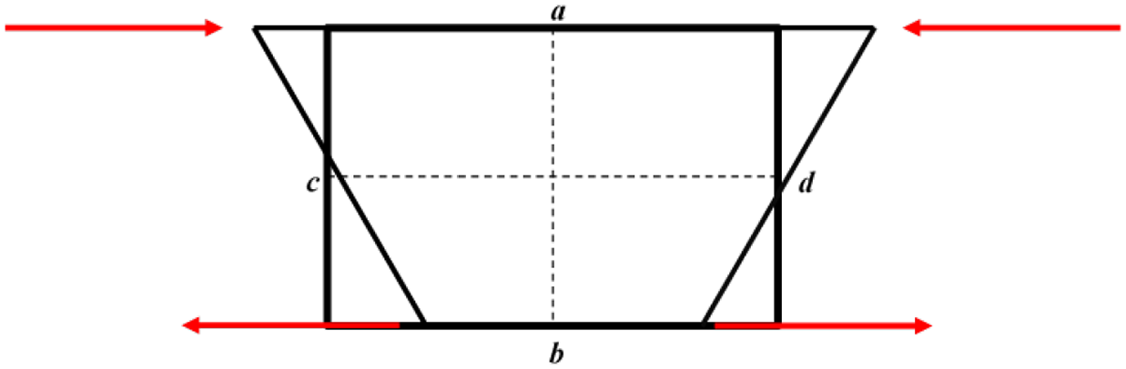
Internal nodal forces counteracting hourglassing.

The other type hourglass control considered for this research was the Belytschko-Bindeman (1993) formulation, known as HG6 within LS-DYNA. This formulation dictates that the material properties of each element are used to calculate an assumed stress field from an assumed strain field. This calculated stress field is integrated over the element domain using a closed form to develop the hourglass forces required for fully-integrated element behavior (LSTC, 2012). After noticing little difference in the computed results among the different considered hourglass algorithms, the authors decided to use the Belytschko-Bindeman formulation for a couple reasons. First, this hourglass type is required for implicit analyses (which the authors used during material model development) and is permitted for explicit analyses (required for the dynamic testing of the rivets to capture the rate-dependent aspects of the solution). Second, LS-DYNA literature (LSTC, 2012) indicates that the Belytschko-Bindeman algorithm is typically more effective than both the viscous and stiffness hourglass controls when dealing with elements that become significantly skewed. With elements in the shaft of the rivet experiencing significant deformation under high shear stresses, choosing the Belytschko-Bindeman proved appropriate for this research.

LS-DYNA warns the user that the Belytschko-Bindeman formulation may artificially stiffen the results and that a reduced hourglass coefficient may be required to minimize this stiffening effect. The research described in this paper used an hourglass coefficient of 0.01, which is a reduction from the default value of 0.1 but is within the LS-DYNA recommended reduced range of 0.001 and 0.01 for solid elements. Checks were made to ensure meaningful hourglass issues were not apparent visually (i.e. no zig-zag distorted deformations) and numerically (hourglass energy was less than 10% of the internal energy for both the whole system via the glstat file (*DATABASE_GLSTAT) and each part via the matsum file (*DATABASE_MATSUM)) within LS-DYNA.

Invariant node numbering was another technique used to avoid element distortion. Rivets under high stresses with large element distortion can cause numerical instability due to reorientation of the element coordinate system, which adversely affects element connectivity. By turning on invariant node numbering within LS-DYNA using *CONTROL_ACCURACY (INN = 3 for solid elements), element rotation calculations were independent of the order of the nodes, and the results were insensitive to the element connectivity. While early models without invariant node numbering provided similar results, selecting this option was strongly recommended for problems with large shear forces (Forsberg, 2013).

With the decision to choose solid elements, loadings and boundary conditions are treated realistically because they are applied on a three-dimensional model without the dimensional simplifications typically required in 1-D and 2-D models associated with using beam and shell elements. In modeling the testing conducted by Rabalais (2015) using a 200-kip dynamic loader, care was required with respect to dictating these support conditions within LS-DYNA. The details and intent of the laboratory setup were critical in determining modeled boundary conditions. Thus, fixed boundary conditions were applied at the plate end in the model to replicate the gripping mechanism system at one of the plate ends in the laboratory testing. Thus, all displacements in three-dimensional space were prohibited from moving (DOFX, DOFY, DOFZ within LS-DYNA under *BOUNDARY_SPC_SET). Similarly, the gripping mechanism system and piston that pulled down on the other end of the riveted plate in the lab was modeled in LS-DYNA by applying a displacement-controlled prescribed motion of that moving end for each analysis. A comparison of the model to the test setup is illustrated in Figure 5.

Figure 5.

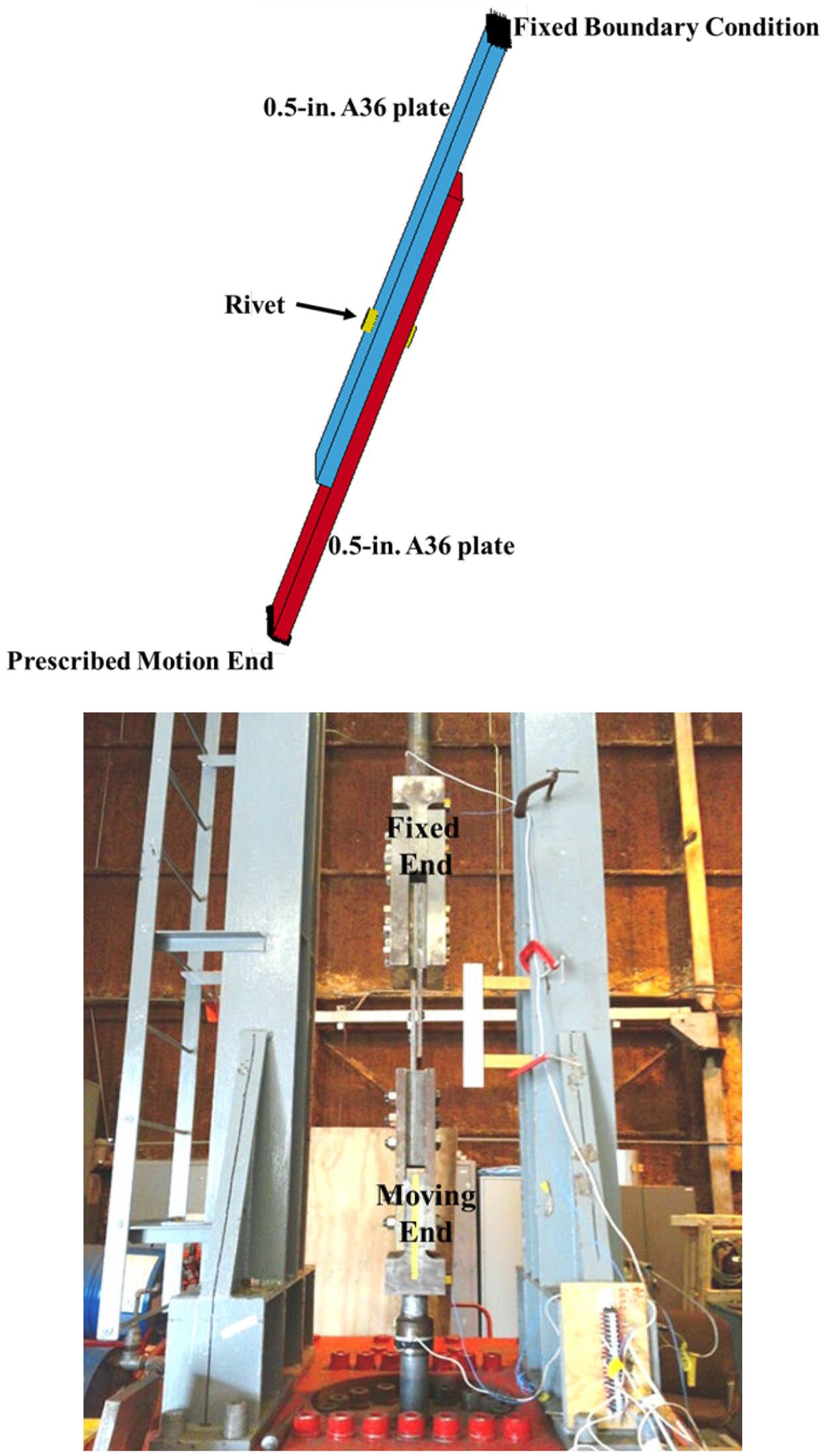
Model setup (top) and laboratory setup (bottom) (photo from Rabalais, 2015).

For initial model validation under quasi-static loading, several analyses were conducted to explore how the computed failure load and behavior compared with the experimental program. A primary goal was to have the finite element model solution compute failure in a manner that accurately represented the experimental tests. Although experimental loading rates were not recorded and differed for each configuration, failure for each rivet under quasi-static loading occurred between 500 and 4000 msec (Rabalais, 2015). For the finite element model, displacement-controlled prescribed motion was applied to each quasi-static test conducted for each configuration in single- and double-shear. This displacement was applied at one end of one plate along one axis (x-translational DOF in LS-DYNA for each model). In some of the more complex cases involving double shear and/or multiple rivets, a slower prescribed motion was used after the initial run indicted a response that reached peak strength faster than what was observed in testing.

Contact within a finite element program allows unmerged elements to interact with each other via impact, sliding, and bearing. In analyses dealing with high strain rates and blast, deformations can be significant. How and where this contact takes place can be extremely difficult to determine. As a result, analyses dealing with high strain rates and blast typically use an automatic contact option. The automatic contact options within LS-DYNA are non-oriented and detect potential penetration from all directions. Described as the most efficient and reliable contact option within LS-DYNA, *CONTACT_AUTOMATIC_SINGLE_SURFACE was used for all analyses (LS-DYNA Support, 2014). Contact was defined by identifying part sets that included the plates and the rivets. During each time step, a search was made to check for potential penetration. A soft constraint-based approach was used (SOFT=1) with the automatic single surface contact option. This modeling approach is recommended for most explicit impact analyses and for situations when dissimilar materials (in this case the A502 Grade 2 rivets with A36 steel) come into contact (LS-DYNA Support, 2014).

In constructing each model, care was taken to place each rivet symmetrically within each plate hole. The manual procedure adopted, however, was not without the possibility of human error. LS-DYNA offers an option within their automatic contacts to offset initial penetration issues by selecting IGNORE=1 via *CONTACT. Another option within LS-DYNA is for the user to input values for static (FS) and dynamic (FD) friction parameters. These parameters affect sliding behavior. Omitting these values tells the software to assume frictionless behavior. Defining both values tells LS-DYNA to consider the relative velocity with which the parts are sliding. There are a wide range of values recommended within different reference manuals, papers, and engineering forums for steel, and these values often depend on the surface conditions. The Civil Engineering Reference Manual (Lindeburg, 2003) recommends values between 0.08 and 0.42 for steel-on-steel contact for FD and between 0.10 and 0.78 for FS. Several combinations of coefficients were used in preliminary analyses, with FD less than FS because it takes more force to accelerate a mass from rest than to keep it moving. Another variable that can influence the amount of noise seen in a computed solution is the viscous contact damping (VDC) parameter. Because contact oscillations between the plates and the rivet(s) can lead to unwanted noise in the response, the VDC parameter within *CONTACT improves model stability and reduces noise. Based on the LS-DYNA guidelines for metals in contact, a value of 20 percent (input as 20, not 0.2 within LS-DYNA) was used throughout all analyses to smooth out response (LS-DYNA Support, 2014).

LS-DYNA has over 130 material models available to simulate a wide range of engineering materials. With a large variety of models to choose from, MAT24, a piecewise-linear plasticity model, was selected because it is widely considered the most popular material model for representing rate-dependent phenomena (Lobo, 2007). MAT24 consists of an elastic-plastic curve defined by the user. Failure occurs when the material reaches a maximum strain from the elastic-plastic curve. With an exhaustive literature search for existing A502 Grade 2 rivet material model parameters turning up empty, the model curve was created by matching milled rivet tension tests from the University of Alabama (Allison, 2015). The rivet coupon model geometry was created using AutoCAD Civil 3D, saved as an .igs file, and imported into LS-PrePost 4.1. A comparison of the meshed rivet tested in LS-DYNA with the experimentally tested rivet is shown in Figure 6.

Figure 6.

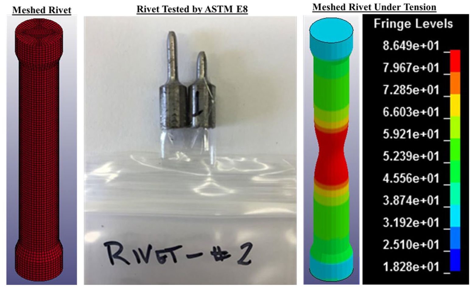
Tested rivet comparison with LS-DYNA analysis (rivet photo from Allison, 2015).

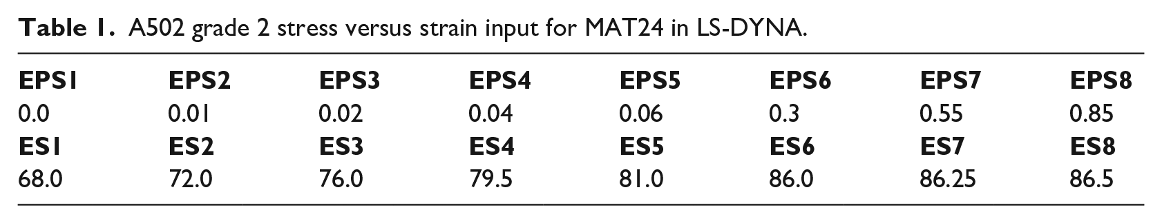
The MAT24 model within LS-DYNA offers a total of eight stress and strain values to define the behavior of the material being modeled. When entering data into LS-DYNA, the stress and strain values must represent true stress and true strain. For the eight stress and strain points within MAT24, the first strain value must be defined as zero to use the input for Young’s Modulus (29,000 ksi). At the onset of necking, a trial-and-error process was used to create the post-necking portion of the true stress versus true strain curve. After making educated guesses on the true stress and true strain values after necking, an analysis simulation was executed. Following the completion of an analysis, the d3plot file was opened within LS-DYNA, and engineering stress versus engineering strain data were plotted. This simulated engineering stress versus engineering strain curve was compared with the experimental engineering stress versus engineering strain curves provided by Allison (2015). The input post-necking stress versus strain values that provided an engineering stress versus engineering strain curve closest to the experimental values was considered the best approximation of the material’s actual stress versus strain relationship. The input values for effective plastic strain, EPS, in units of in./in. and corresponding yield stress, ES, in units of ksi that most closely matched the experimental behavior is shown in Table 1.

Table 1.

A502 grade 2 stress versus strain input for MAT24 in LS-DYNA.

EPS1	EPS2	EPS3	EPS4	EPS5	EPS6	EPS7	EPS8
0.0	0.01	0.02	0.04	0.06	0.3	0.55	0.85
ES1	ES2	ES3	ES4	ES5	ES6	ES7	ES8
68.0	72.0	76.0	79.5	81.0	86.0	86.25	86.5

At this point in the simulation, and as shown in Figure 7 as the “Coarsest Mesh,” the simulated engineering stress versus engineering strain curve was not acceptably accurate. Thus, an attempt was made to refine the mesh to increase accuracy. Mesh convergence was conducted by plotting simulated engineering stress versus engineering strain using the input from Table 1 for each mesh size and comparing it against the experimental engineering stress versus engineering strain plots. Several simulations were run to achieve convergence. Local mesh refinement in the middle third of the rivet coupon was considered; however, with the desire to use the same mesh density range for the rivet models, the decision was made to maintain a consistent mesh density throughout the entire coupon. This decision also prevented potential issues with misrepresented geometry and unsuitable mesh transitions, which could adversely affect accuracy. Figure 7 shows the engineering stress versus engineering strain results for a sample of the mesh sizes analyzed. As the mesh size decreased, the accuracy of the simulated engineering stress versus engineering strain curve improved to the point of approximating the experimental tension test results.

Figure 7.

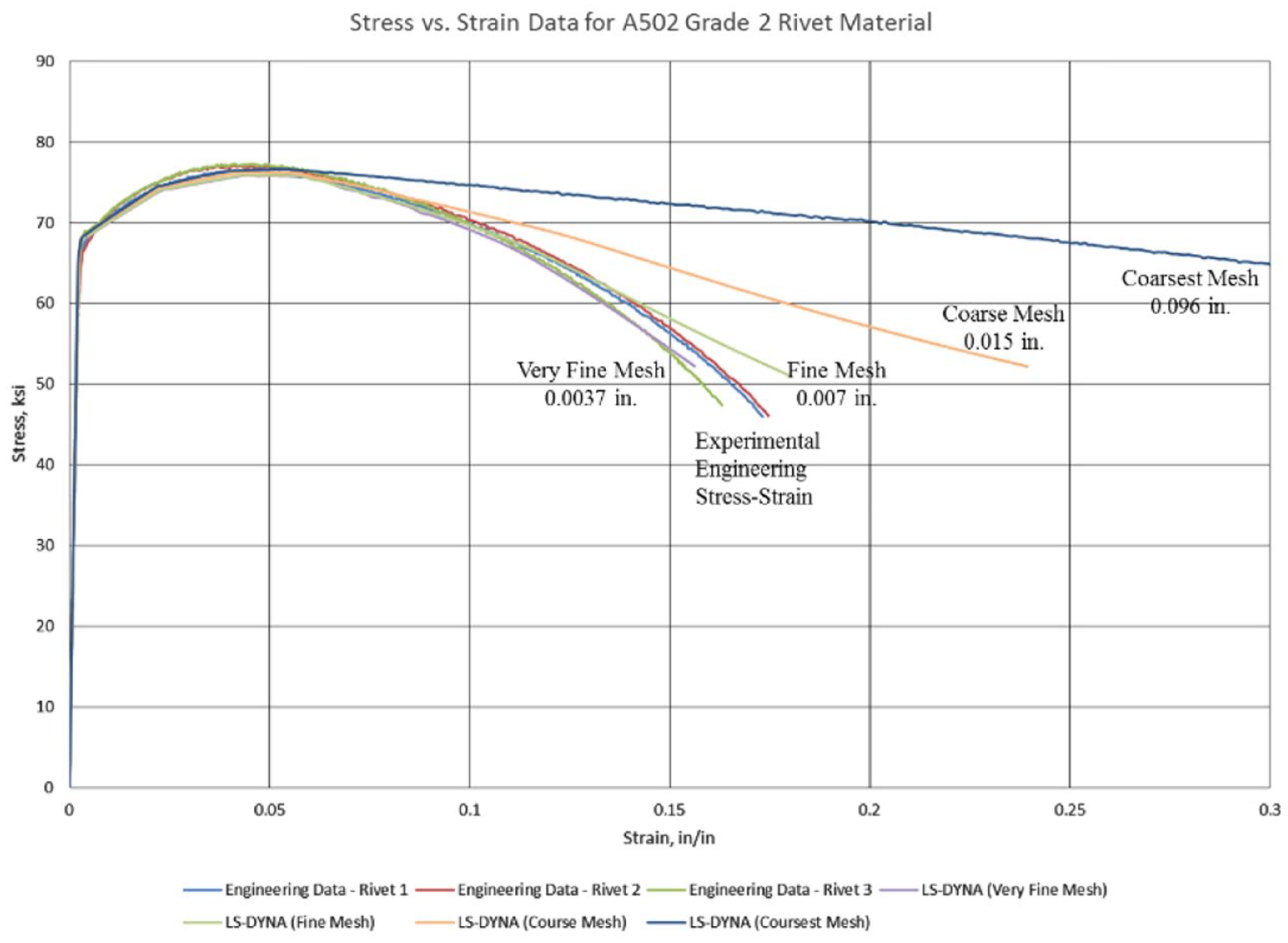
Results of mesh sensitivity analysis for tension testing.

Satisfied with the convergence of the tension coupon model, initial models for shear consisted of an analysis of Configuration 1 (one single rivet) in single shear using a mesh size of 0.0037-in for the rivet. This mesh size corresponded with the one that best approximated the engineering stress versus engineering strain curve obtained from experimental testing. Despite its accuracy, the computational demand of this mesh size was extremely high and deemed unnecessary to achieve the desired level of accuracy. Consequently, the authors used a coarser mesh, balancing computation demand with execution time, for subsequent models. A sample of the subsequent mesh sensitivity study for rivets in shear is shown in Figure 8. In each case, a successive level of mesh refinement involved splitting the elements of the previous model in all directions. In comparing the meshes from Figure 8 with the mesh size samples from the coupon tension tests from Figure 7, Mesh A corresponds with the Coarsest Mesh results, Mesh B corresponds with an analysis between the Coarsest Mesh and the Coarse Mesh, Mesh C corresponds with the Coarse Mesh results, and Mesh D corresponds with the Fine Mesh results.

Figure 8.

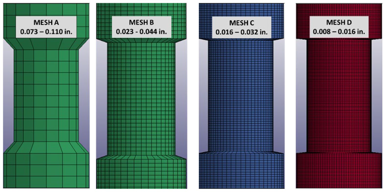
Sample of mesh sensitivity of rivets in shear.

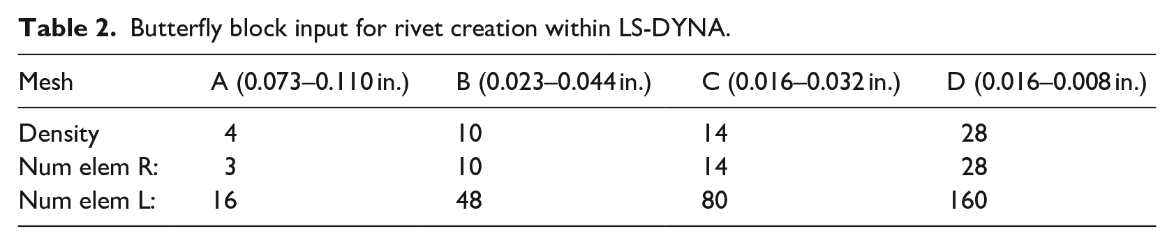
Rivets were created within LS-Prepost by way of butterfly blocks, a three-dimensional automatic solid block mesh with 6 DOF per node (2014). For rivets in single shear, a radius of 0.28125-in. was selected to represent the rivet completely filling the hole. For subsequent testing involving double shear, a reduced radius of 0.2725-in. was used to replicate the rivet material not completely filling the hole. The radius used for these analyses was consistent with the findings of Rabalais (2015). Single-shear rivets had a length of 1.6-in., and the double-shear rivets had a length of 2.6-in. The center 1-in. or 2-in. of the rivet shaft corresponded to the two 0.5-in. thick plates used in single-shear testing, and the two 0.5-in. thick and one 1-in. thick plate used in double-shear testing, respectively. The remaining 0.6-in. was used to simulate a head on each end of the rivet. The additional input used to create the rivets in single shear using the block mesher butterfly block method is shown in Table 2. The terms “Num Elem R” and “Num Elem L” within the table represent the number of elements in the R and L directions of the cylinder as shown in Figure 9. Simulations were run in the multi-node Ferguson Structural Engineering Lab at The University of Texas at Austin. Each node comprising the File Allocation Table facility contains a Dell PowerEdge R820 server, 256 GB RAM, 32 cores (@2.4 GHz, 614.4 gigaflops).

Table 2.

Butterfly block input for rivet creation within LS-DYNA.

Mesh	A (0.073–0.110 in.)	B (0.023–0.044 in.)	C (0.016–0.032 in.)	D (0.016–0.008 in.)
Density	4	10	14	28
Num elem R:	3	10	14	28
Num elem L:	16	48	80	160

Figure 9.

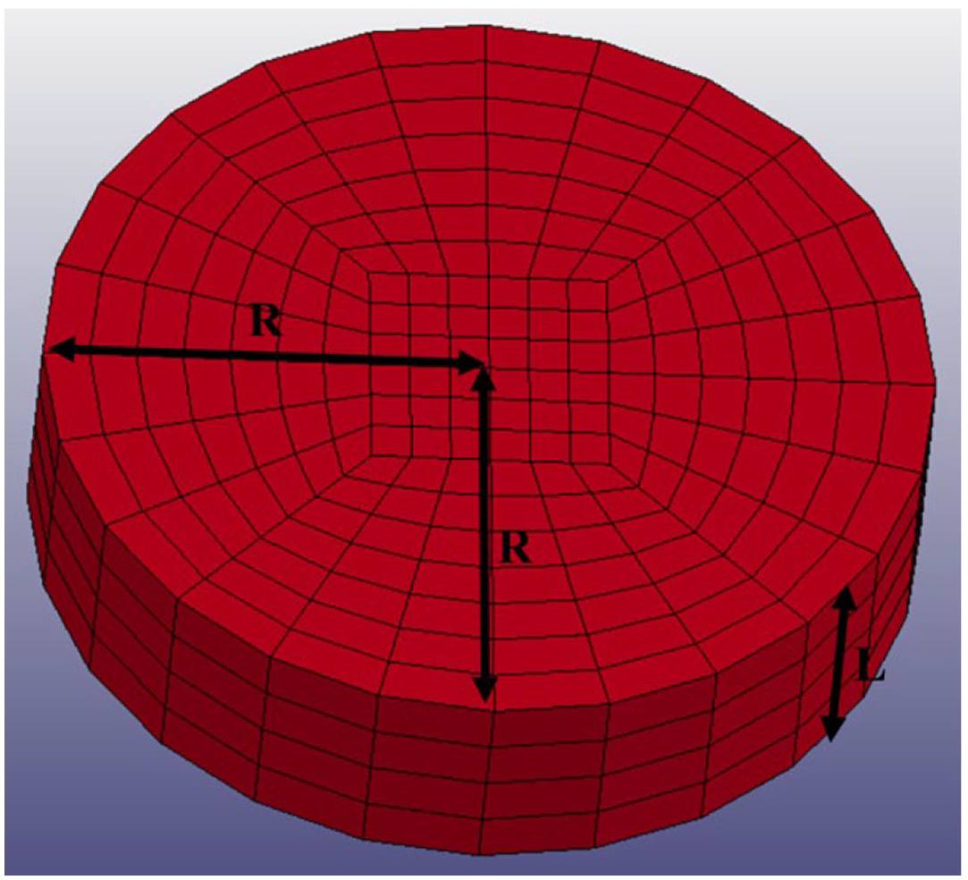
Butterfly block creation template (from LSTC, 2012).

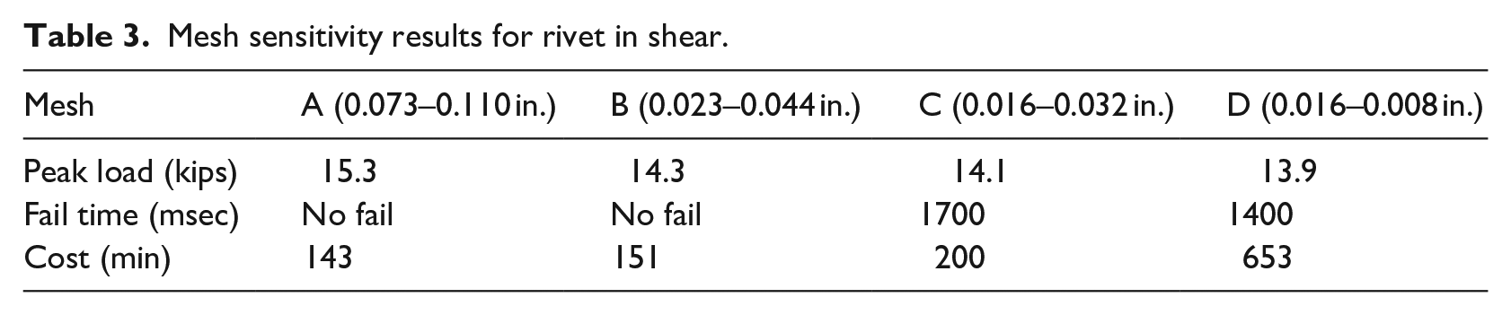
Results from this mesh sensitivity study, summarized in Table 3, provided valuable information with respect to modeling rivets in shear. First, the peak load results for each test fell within the expected values. For an average experimental tensile strength of 77 ksi, the expected shear strength is 0.75 times the tensile strength times the rivet area of 0.2485 in², or 14.35 kips. As shown in Figure 11 and Table 3, the peak load for each mesh simulation was within 1 kip of the anticipated value and was well within the range of the experimental data, represented by curves RS1S1, RS1S2, RS1S3, and RS1S4. In fact, regardless of the mesh size, there was very little scatter in the simulated results with respect to shear strength, as the data varied by only 1.4 kips. As a point of comparison, this difference in peak load between mesh sizes is approximately one-third of the range of the experimental data (16.7 kips maximum value and 12.6 kips minimum value).

Table 3.

Mesh sensitivity results for rivet in shear.

Mesh	A (0.073–0.110 in.)	B (0.023–0.044 in.)	C (0.016–0.032 in.)	D (0.016–0.008 in.)
Peak load (kips)	15.3	14.3	14.1	13.9
Fail time (msec)	No fail	No fail	1700	1400
Cost (min)	143	151	200	653

The primary difference in response based on mesh size was in the computed ductility, which was consistent with what was observed during the tension test simulations. As the rivet material coupon’s mesh size decreased, the accuracy with respect to ductility improved significantly. This same pattern is demonstrated in Figure 10. With the coarser mesh sizes from Mesh A (0.073–0.110 in.) and Mesh B (0.023–0.044 in.), the rivets demonstrated unrealistic ductility. With the finer mesh sizes of Mesh C (0.016–0.032 in.) and Mesh D (0.008–0.016 in.), however, the rivets demonstrated reasonable ductility consistent with the experimental results.

Figure 10.

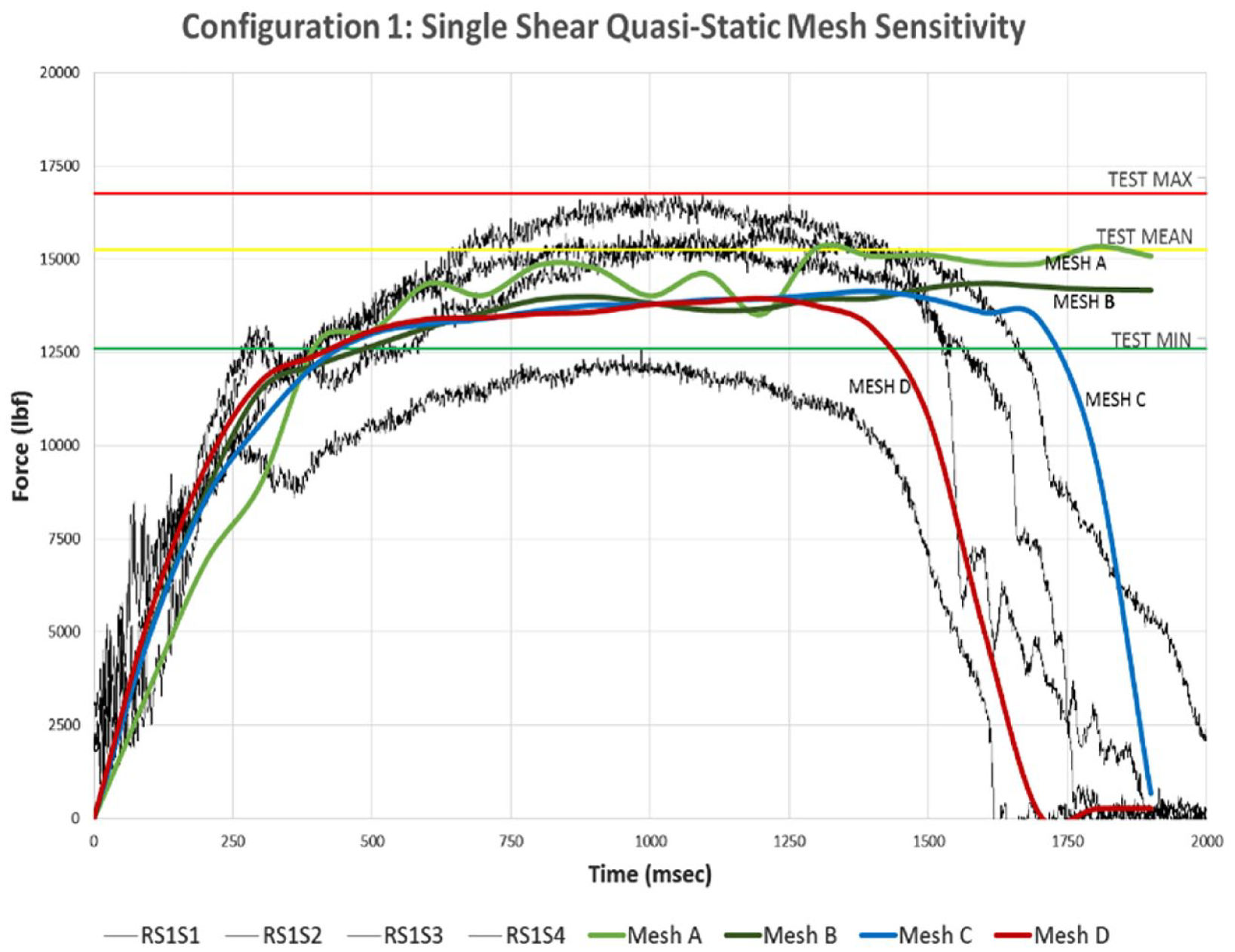
Illustration of mesh sensitivity study for one rivet in single shear.

The mesh sensitivity study not only showed important revelations with respect to ultimate shear strength and ductility, it also revealed critical information with respect to computational cost. As expected, the amount of time it took to process each model was dependent on the mesh size of the rivet. The finest mesh size tested, Mesh D, took more than three times as long to run as the other mesh sizes; whereas, there was a relatively insignificant difference in cost for the other mesh sizes. With Mesh C and Mesh D providing similar results with respect to maximum shear stress and ductility, subsequent analyses were conducted with these meshes. Given the wide variability in the behavior of rivets, engineering judgement suggests it is perfectly fine to have acceptable accuracy considering real bridges with real rivets would undoubtedly demonstrate a great deal of scatter.

The riveting process involves heating and cooling of the rivets and results in the development of residual forces that clamp plates together, and the authors considered trying to capture these residual forces in the model. However, previous research by Wallaert and Fisher (1962), Higgins and Ruble (1955), Munse et al. (1956), Kaplan (1959), and Bendigo et al. (1963) concluded that the amount of pre-tension in fasteners had no effect on their ultimate shear strength. These researchers concluded that regardless of the number of fasteners, how they were configured, the number of shear planes, or the strength of the individual fasteners, the amount of tension developed during installation had an insignificant effect on the fastener’s ultimate shear strength. Thus, with all analyses focused on the ultimate behavior of rivets under shear loading, the authors decided to ignore the effects of thermally induced residual forces in the rivet.

Quasi-static simulation results

The material model used for analysis within LS-DYNA was based on a conservative estimate of the tensile strength of the rivet material before the riveting process. The process of installing a rivet can increase the tensile and shear strength by 10–20 percent (Kulak et al., 1987). With this inherent variance, the authors decided to use the more conservative model, providing the engineering community with a reasonable depiction of rivet behavior without artificially changing the validated material model. However, it must be acknowledged that although the tensile and shear strengths increase during the riveting process, the ductility decreases (Collette et al., 2016). Thus, the properties of the rivet material before the riveting process are not always conservative.

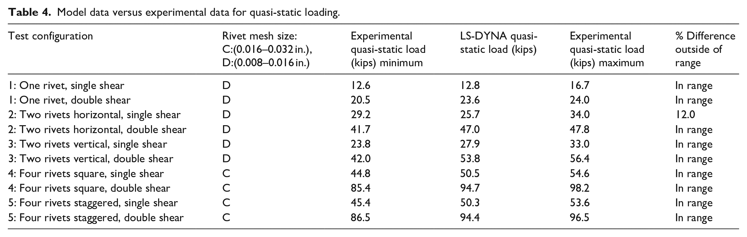
Table 4 provides the model data versus the experimental data for quasi-static loading. In nine of the 10 quasi-static rivet model simulations, the LS-DYNA prediction for maximum shear strength fell within the range of the experimentally measured shear strength values. In the one simulation that fell outside the range of the experimentally measured shear strength values (two horizontal rivets in single shear), the model provided a reasonable representation of the rivet behavior by underestimating capacity by only 12%. While already reasonable, a 10–20 percent increase in the material model input to account for the riveting process would have adjusted the simulation result to fall within the experimental range. In addition, the results of each simulation revealed an acceptably accurate comparison to the experimental results with respect to time to failure.

Table 4.

Model data versus experimental data for quasi-static loading.

Test configuration	Rivet mesh size: C:(0.016–0.032 in.), D:(0.008–0.016 in.)	Experimental quasi-static load (kips) minimum	LS-DYNA quasi-static load (kips)	Experimental quasi-static load (kips) maximum	% Difference outside of range
1: One rivet, single shear	D	12.6	12.8	16.7	In range
1: One rivet, double shear	D	20.5	23.6	24.0	In range
2: Two rivets horizontal, single shear	D	29.2	25.7	34.0	12.0
2: Two rivets horizontal, double shear	D	41.7	47.0	47.8	In range
3: Two rivets vertical, single shear	D	23.8	27.9	33.0	In range
3: Two rivets vertical, double shear	D	42.0	53.8	56.4	In range
4: Four rivets square, single shear	C	44.8	50.5	54.6	In range
4: Four rivets square, double shear	C	85.4	94.7	98.2	In range
5: Four rivets staggered, single shear	C	45.4	50.3	53.6	In range
5: Four rivets staggered, double shear	C	86.5	94.4	96.5	In range

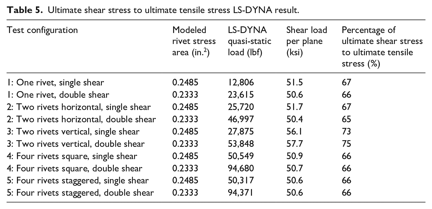
A further look at the LS-DYNA analysis results revealed that both the ultimate shear strength and the ratio of ultimate-shear-strength-to-ultimate-tensile-strength for each configuration were reasonable. Based on historical data collected and reported in the Guide to Design Criteria for Bolted and Riveted Connections (Kulak et al., 1987) and the ultimate tensile strength of the rivet coupon for this research, expectations were that the ultimate shear strength of the rivets would range between 53 ksi and 66 ksi. The shear load per plane demonstrated by the rivet and material model created from this research ranged from 50.4 ksi to 57.7 ksi. Any increase to the material model input to account for the riveting process would have likely fit the expected data even better. Furthermore, the Guide to Design Criteria for Bolted and Riveted Connections (Kulak et al., 1987) revealed the average shear-to-tensile strength ratio for rivets varied from 0.67 to 0.83, with an average of 0.75. Table 5 reveals that the ultimate-shear-strength-to-ultimate-tensile-strength ratio, ranging from 0.65 to 0.75 from this LS-DYNA research, provided a reasonable response that was consistent with historical data. This percentage was calculated by comparing the shear load per plane from the LS-DYNA analysis results to the ultimate tensile strength obtained from the LS-DYNA coupon tests (77 ksi).

Table 5.

Ultimate shear stress to ultimate tensile stress LS-DYNA result.

Test configuration	Modeled rivet stress area (in.²)	LS-DYNA quasi-static load (lbf)	Shear load per plane (ksi)	Percentage of ultimate shear stress to ultimate tensile stress (%)
1: One rivet, single shear	0.2485	12,806	51.5	67
1: One rivet, double shear	0.2333	23,615	50.6	66
2: Two rivets horizontal, single shear	0.2485	25,720	51.7	67
2: Two rivets horizontal, double shear	0.2333	46,997	50.4	65
3: Two rivets vertical, single shear	0.2485	27,875	56.1	73
3: Two rivets vertical, double shear	0.2333	53,848	57.7	75
4: Four rivets square, single shear	0.2485	50,549	50.9	66
4: Four rivets square, double shear	0.2333	94,680	50.7	66
5: Four rivets staggered, single shear	0.2485	50,317	50.6	66
5: Four rivets staggered, double shear	0.2333	94,371	50.6	66

As a final but important aspect used to assess the validity of the modeling approach for this research, a close investigation of the three-dimensional rivet models following the quasi-static simulations was conducted. The fracture type and deformed shape changes significantly based on the loading type (shear, tension, or combination of both). Under pure shear deformation, as was the intent of the models for this research, necking should not occur. As illustrated in Figure 11 (and similarly for each of the 10 quasi-static LS-DYNA simulations), no necking was evident in the fracture of the rivets, providing further confidence in the computational models developed for this research. Conversely, the models did capture necking when they corresponded to the case of pure tension.

Figure 11.

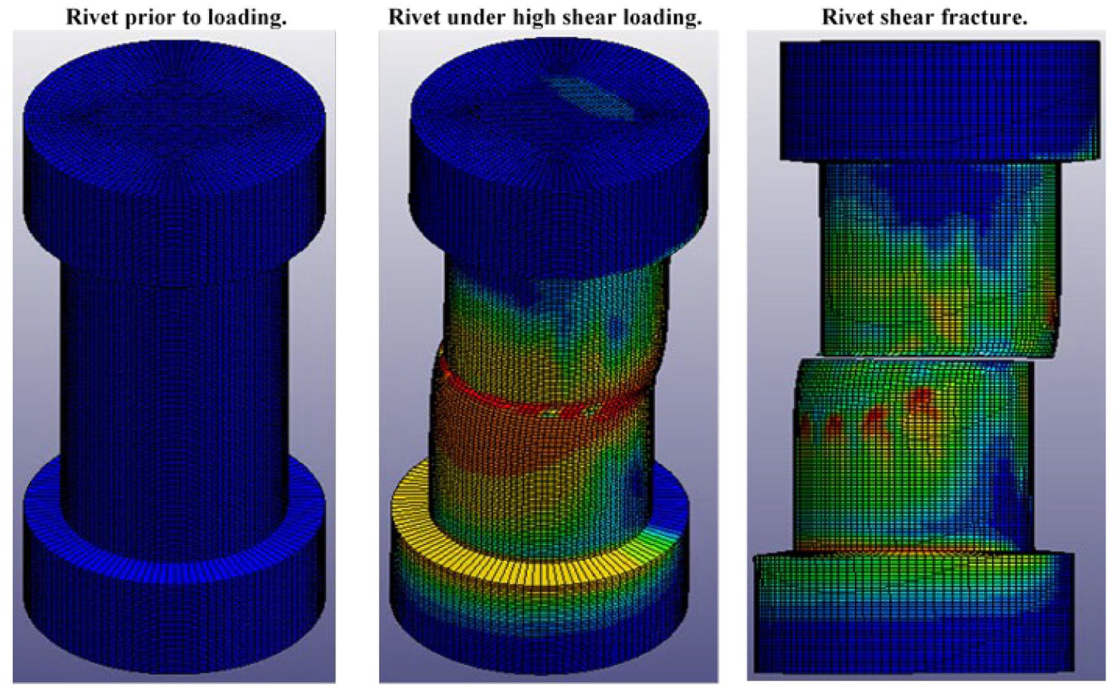
Illustration of shear fracture of LS-DYNA mode.

Modeling high rates of loading

The Johnson-Cook (1985) and Cowper Symonds (1957) are two popular constitutive models used to capture strain-rate effects in ductile metals. The Johnson-Cook model is available as an option within LS-DYNA as *MAT_TABULATED_JOHNSON_COOK (MAT 224) to capture rivet behavior under high loading rates. This model uses a table of curves that defines plastic failure strain as a function of triaxiality, strain rate, temperature, and element size. The development of plastic strain input curves requires the execution of a series of tension tests under various strain rates and temperatures. When compared to the Johnson-Cook model, the Cowper Symonds constitutive model is simple in that it captures the differences between dynamic and static load effects ( $σ_{Y d}$ , yield stress under dynamic loads, versus $σ_{Y}$ , yield stress under quasi-static loads) through the strain rate ( $\dot{ε}$ ) and two empirical coefficients (C, q) that traditionally are determined through experimental testing. Furthermore, the Cowper Symonds constitutive model provides a great advantage to the quasi-static modeling completed because it is incorporated into the piecewise-linear plasticity material model (MAT24) through a user input of the two empirical coefficients and the material’s true stress-strain curve (equation (1)).

σ_{Y d} = σ_{Y} + σ_{Y} {(\frac{\dot{ε}}{C})}^{\frac{1}{q}}

(1)

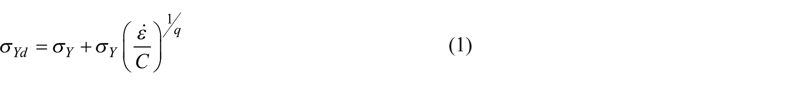
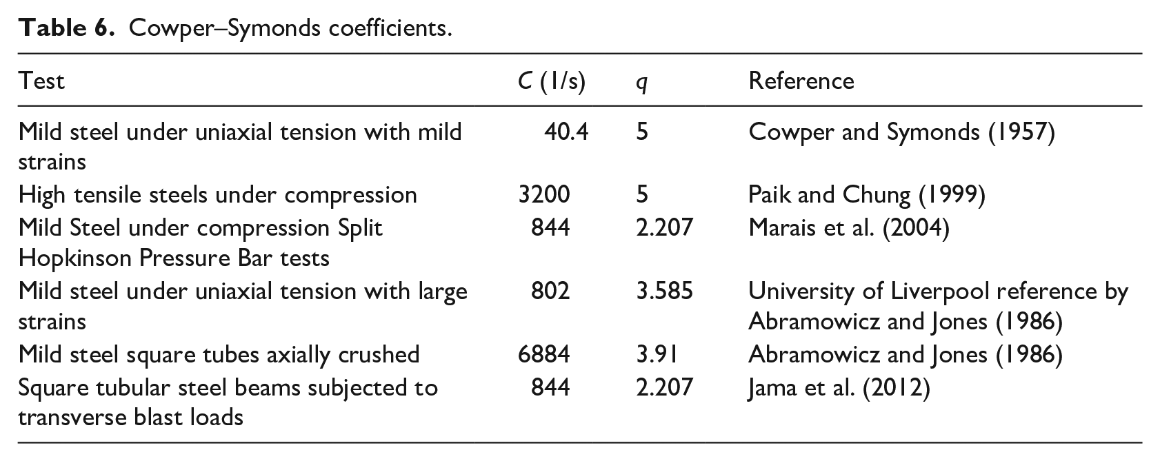
Unable, to find Cowper Symonds empirical coefficients for A502 Grade 2 rivets or any other steel rivet type reported, the authors researched testing that generated empirical values of C and q for mild steel. In analyzing these values, shown in Table 6, it was evident that the empirical value q was relatively consistent for all mild steel dynamic testing, ranging from 2.2 to 5. Conversely, the empirical value C demonstrated a large variability, with values ranging from 40.4 to 6884. The large difference in parameter values and the considerable scatter in published experimental data suggested there were several factors contributing to the behavior of mild steel under high strain rates. These factors included the amount of dynamic strain (elastic behavior versus plastic behavior), loading differences (tension versus compression versus shear), testing techniques, and material composition. With such a large number of contributing variables, the authors compared experimental test results with computed results using extreme values for C and q within LS-DYNA.

Table 6.

Cowper–Symonds coefficients.

Test	C (1/s)	q	Reference
Mild steel under uniaxial tension with mild strains	40.4	5	Cowper and Symonds (1957)
High tensile steels under compression	3200	5	Paik and Chung (1999)
Mild Steel under compression Split Hopkinson Pressure Bar tests	844	2.207	Marais et al. (2004)
Mild steel under uniaxial tension with large strains	802	3.585	University of Liverpool reference by Abramowicz and Jones (1986)
Mild steel square tubes axially crushed	6884	3.91	Abramowicz and Jones (1986)
Square tubular steel beams subjected to transverse blast loads	844	2.207	Jama et al. (2012)

LS-DYNA simulations were conducted for every experimentally tested rivet configuration using the published bounding empirical values of the original Cowper Symonds parameters (C = 40.4 s⁻¹ and q = 5) and the Abramowicz and Jones parameters (C = 6884 s⁻¹ and q = 3.91). The Cowper Symonds parameters were derived from experimental testing involving mild steel loaded axially in tension, while the Abramowicz and Jones parameters were obtained from experiments involving the dynamic axial crushing of mild steel tubes.

Of all the LS-DYNA parameters and settings validated and described earlier in this paper, only the prescribed motion curve input required modification to impose dynamic loading. As with the quasi-static loading analysis, several simulations were required to get the rivet to fail dynamically in a mode similar to the experiments. The primary challenge in developing these models was in defining the load rates, which were not precisely measured during the experimental testing program (Rabalais, 2015). Although attempts were made to control the rate of loading during the testing program, doing so proved to be exceptionally difficult, and actual loading rates varied among the specimens (Rabalais, 2015). Experimentally, failure for each rivet under dynamic loading occurred in less than 7 msec. This time benchmark, in conjunction with the general shape of the load-versus-time curves, served as the basis for qualitative acceptance of the computed results.

Dynamic simulation results

The Cowper Symonds (C = 40.4 s⁻¹ and q = 5) and Abramowicz and Jones parameters (C = 6884 s⁻¹ and q = 3.91) predicted reasonable rivet behavior under dynamic loads in LS-DYNA despite serving as bounding values for published recommended parameters. The results of the 10 LS-DYNA simulations of dynamic response for each set of parameters (C = 40.4 s⁻¹ and q = 5 versus C = 6884 s⁻¹ and q = 3.91) are shown in Tables 7 and 8. Positive percentages from indicate LS-DYNA models that provided an ultimate shear strength greater than the experimental test results while negative percentages indicate the LS-DYNA model provided an ultimate shear strength less than the experimental test results (Rabalais, 2015).

Table 7.

Dynamic loading simulation results using Cowper Symonds parameters (C = 40.4 s⁻¹ and q = 5) versus experimental results.

Test configuration	Rivet mesh size: C: (0.016.−0.032 in.), D: (0.008 in.−0.016 in.)	Experimental dynamic load (kips) minimum	Experimental dynamic load (kips) maximum	LS-DYNA dynamic load (kips), C = 40.4 s⁻¹ and q = 5.27	% Difference outside of range
1: One rivet, single shear	D	13.7	16.1	27.3	40.8
1: One rivet, double shear	D	31.0	44.7	47.4	5.6
2: Two rivets horizontal, single shear	D	39.4	79.6	50.2	In range
2: Two rivets horizontal, double shear	D	55.9	85.5	105.2	18.7
3: Two rivets vertical, single shear	D	54.2	60.3	49.7	-8.3
3: Two rivets vertical, double shear	D	79.8	132.6	103.0	In range
4: Four rivets square, single shear	C	54.4	117.4	106.9	In range
4: Four rivets square, double shear	C	102.9	147.8	193.1	23.4
5: Four rivets staggered, single shear	C	66.4	94.5	101.0	6.5
5: Four rivets staggered, double shear	C	147.6	213.2	176.6	In range

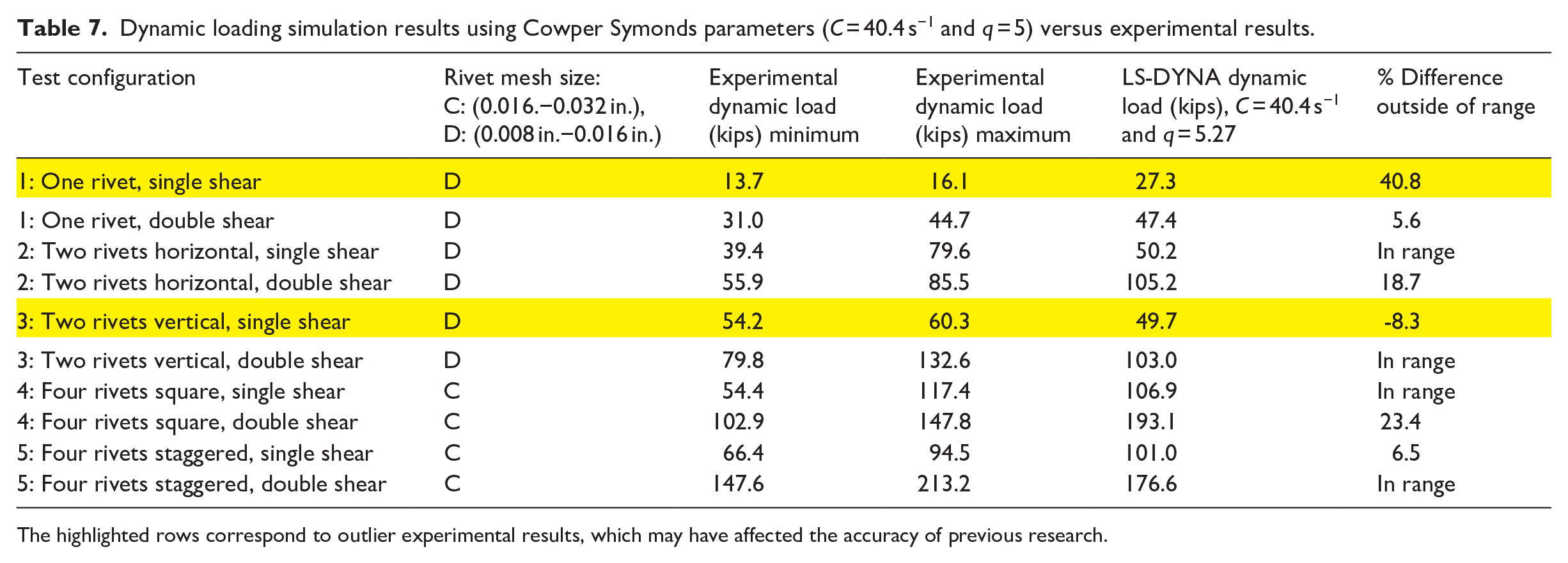
The highlighted rows correspond to outlier experimental results, which may have affected the accuracy of previous research.

Table 8.

Dynamic loading simulation results using Abramowicz and Jones (1986) parameters (C = 6884 s⁻¹ and q = 3.91) versus experimental result.

Test configuration	Rivet mesh size: C: (0.016–0.032 in.), D: (0.008 in.−0.016 in.)	Experimental dynamic load (kips) minimum	Experimental dynamic load (kips) maximum	LS-DYNA dynamic load (kips), C = 6884 s⁻¹ and q = 3.91	% Difference outside of range
1: One rivet, single shear	D	13.7	16.1	18.5	12.9
1: One rivet, double shear	D	31.0	44.7	30.9	−0.2
2: Two rivets horizontal, single shear	D	39.4	79.6	33.8	−14.2
2: Two rivets horizontal, double shear	D	55.9	85.5	64.0	In range
3: Two rivets vertical, single shear	D	54.2	60.3	31.9	−41.1
3: Two rivets vertical, double shear	D	79.8	132.6	70.1	−12.1
4: Four rivets square, single shear	C	54.4	117.4	71.3	In range
4: Four rivets square, double shear	C	102.9	147.8	116.3	In range
5: Four rivets staggered, single shear	C	66.4	94.5	65.1	−1.9
5: Four rivets staggered, double shear	C	147.6	213.2	123.5	−16.3

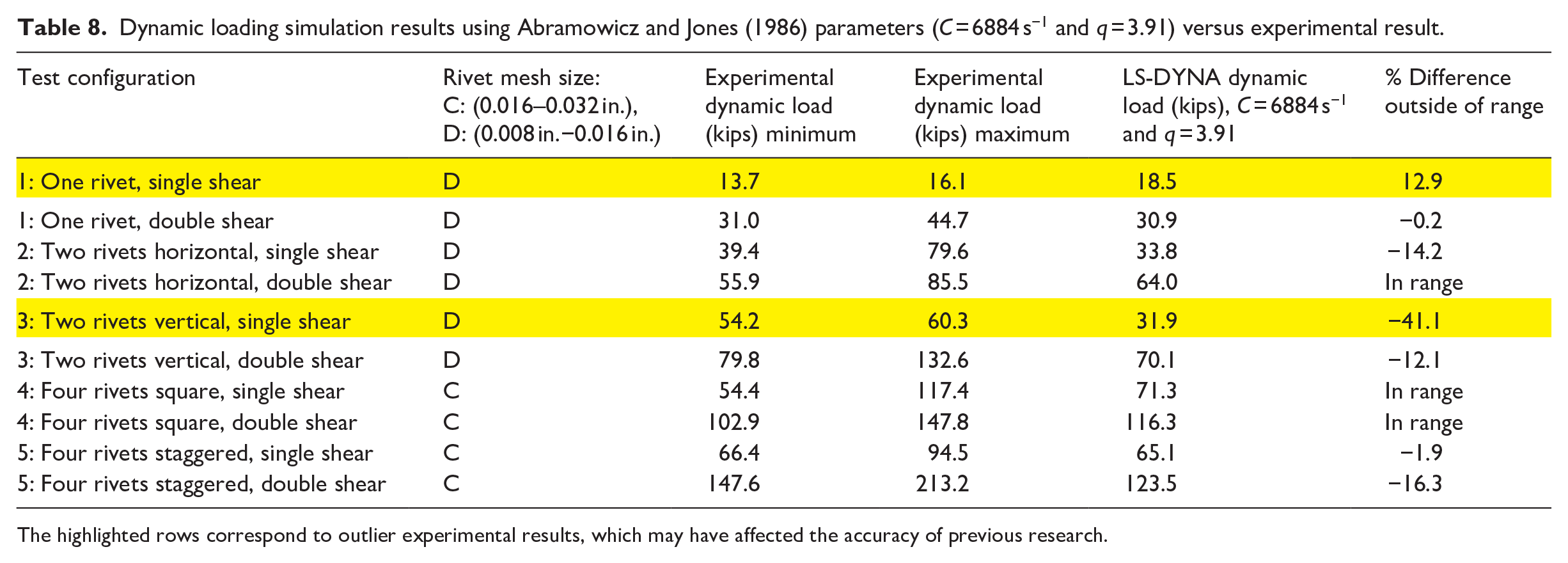
The highlighted rows correspond to outlier experimental results, which may have affected the accuracy of previous research.

In comparing the LS-DYNA results with the experimental results, it is first important to point out two anomalies in the experimental output. While reporting a dynamic increase factor of approximately 1.72 for the rivets, two of the configurations tested experimentally produced dynamic increase factors different than predicted (Rabalais, 2015). Likely contributors to these outlier experimental tests were internal flaws in the riveted plates and the variable nature of dynamic loading. The redistribution of loads within materials can result in a premature failure when flaws exist because the loads will find the weakest point. For Configuration 1 (one rivet in single shear), the anticipated ultimate shear strength based on a 1.72 dynamic increase factor ranged from 21.7 kips to 28.8 kips; however, the measured experimental values were much lower, ranging from 13.7 kips to 16.1 kips. When comparing the LS-DYNA results with the experimental and predicted results, the originally published recommended parameters C = 40.4 s⁻¹ and q = 5 demonstrated an ultimate shear strength that was within range of the predicted values. The parameters of C = 6884 s⁻¹ and q = 3.91, however, provided an ultimate shear strength within LS-DYNA that was approximately 14 percent below the predicted ultimate shear strength. Similarly, for Configuration 3 (two rivets vertical, single shear) the anticipated ultimate shear strength ranged from 40.8 kips to 56.8 kips. Meanwhile, the actual experimental test values were higher, ranging from 54.2 kips to 60.3 kips. The LS-DYNA results for this configuration exhibited a similar trend. The Cowper Symonds recommended parameters input within LS-DYNA produced an ultimate shear stress within the projected range, while the Abramowicz and Jones parameters input within LS-DYNA produced an ultimate shear stress approximately 20 percent below the projected range.

Regarding the remaining eight simulated dynamic rivet models, the parameters C = 40.4 s⁻¹ and q = 5 input within LS-DYNA predicted an ultimate shear strength within the range of the experimental ultimate shear strength 50 percent of the time. The half that fell outside the range overpredicted the shear strength by as much as 23.5 percent. When using the parameters C = 6884 s⁻¹ and q = 3.91, the rivet configurations demonstrated an ultimate shear strength within the range of the experimental ultimate shear strength 37.5 percent of the time. Those that fell outside the range underpredicted the shear strength by as much as 16.3 percent. A summary of all the testing results are shown in Tables 7 and 8, with the previously mentioned outlier experimental test results highlighted in yellow.

For both sets of parameters, the Cowper Symonds constitutive model provided reasonable representations of rivet behavior under dynamic loads. However, the parameters recommended by Cowper Symonds (C = 40.4 s⁻¹ and q = 5) overestimated the strength of the rivets in several cases, which was unconservative given the already variable nature and behavior of rivets. Meanwhile, the Abramowicz and Jones parameters (C = 6884 s⁻¹ and q = 3.91) provided a conservative estimate of the ultimate shear strength in cases where it was not within the range of the experimental values. Recall, also, that the material model for this research, described earlier in this paper, was based on the stress and strain relationship of the rivet steel prior to the riveting process. It is reasonable to expect a 10 to 20 percent increase in the material model input to account for the riveting process, which would adjust the Abramowicz and Jones simulation results to increase within the range of the experimental values. The load versus time curves from all LS-DYNA simulations demonstrated comparable shapes and end times to their experimental counterparts. The different Cowper Symonds parameters had little impact on the overall shape of the curves.

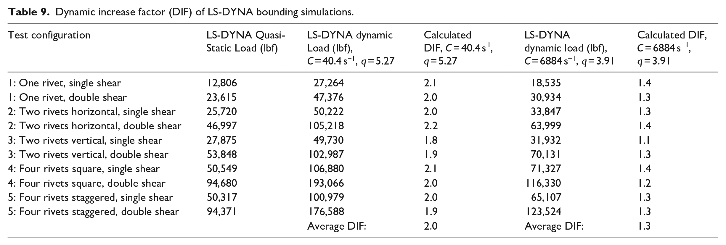
A subsequent analysis of the simulations examined the dynamic increase factor exhibited for each set of Cowper Symonds parameters. This analysis was done by comparing the LS-DYNA output from quasi-static simulations and comparing them to the LS-DYNA output from dynamic simulations. In doing so, it was determined that the parameters C = 40.4 s⁻¹ and q = 5 overestimated the dynamic increase factor of the rivets. As demonstrated in Table 9, the average dynamic increase factor within LS-DYNA was 2.0. Meanwhile, the average dynamic increase factor using the parameters C = 6884 s⁻¹ and q = 3.91 within LS-DYNA was 1.3. As a point of comparison, the dynamic increase factor from the experimental testing, calculated by dividing the mean of the dynamic tests by the mean of the static tests, was 1.7 (Rabalais, 2015). Thus, the Cowper Symonds (C = 40.4 s⁻¹ and q = 5) and Abramowicz and Jones parameters (C = 6884 s⁻¹ and q = 3.91) provided reasonable upper and lower bounds, respectively, of rivet response under high loading rates.

Table 9.

Dynamic increase factor (DIF) of LS-DYNA bounding simulations.

Test configuration	LS-DYNA Quasi-Static Load (lbf)	LS-DYNA dynamic Load (lbf), C = 40.4 s⁻¹, q = 5.27	Calculated DIF, C = 40.4 s¹, q = 5.27	LS-DYNA dynamic load (lbf), C = 6884 s⁻¹, q = 3.91	Calculated DIF, C = 6884 s⁻¹, q = 3.91
1: One rivet, single shear	12,806	27,264	2.1	18,535	1.4
1: One rivet, double shear	23,615	47,376	2.0	30,934	1.3
2: Two rivets horizontal, single shear	25,720	50,222	2.0	33,847	1.3
2: Two rivets horizontal, double shear	46,997	105,218	2.2	63,999	1.4
3: Two rivets vertical, single shear	27,875	49,730	1.8	31,932	1.1
3: Two rivets vertical, double shear	53,848	102,987	1.9	70,131	1.3
4: Four rivets square, single shear	50,549	106,880	2.1	71,327	1.4
4: Four rivets square, double shear	94,680	193,066	2.0	116,330	1.2
5: Four rivets staggered, single shear	50,317	100,979	2.0	65,107	1.3
5: Four rivets staggered, double shear	94,371	176,588	1.9	123,524	1.3
		Average DIF:	2.0	Average DIF:	1.3

While the investigated parameters adequately bounded the ultimate shear strength, a goal of this research was to recommend one set of Cowper Symonds parameters for future research. In taking a closer look at previous testing published in the research literature, greater consideration was given to Cowper Symonds parameters derived from experimental studies most closely aligned with the research presented in this manuscript. Thus, because a correlative relationship exists between the behavior of rivets under tensile loading and rivets under shear loading, historical testing, such as original uniaxial dynamic tensile testing of mild steel from Cowper Symonds, is a priority for consideration (C = 40.4 s⁻¹ and q = 5). Of note, however, is the fact that subsequent uniaxial dynamic tensile testing of mild steel by the University of Liverpool (referred to in Abramowicz and Jones, 1986) provided drastically different results (C = 802 s⁻¹ and q = 3.585). The marked difference between the two cases with respect to testing is that the Cowper Symonds (1956) experiments involved subjecting mild steel specimens to relatively small strains in the neighborhood of their yield value, while the University of Liverpool tests involved subjecting mild steel specimens to relatively large strains and plastic behavior. This observation, in conjunction with noticing the University of Liverpool parameters would likely provide ultimate shear strengths between the bounded values, led to running LS-DYNA simulations of the five configurations in single- and double-shear with the published University of Liverpool parameters (C = 802 s⁻¹ and q = 3.585).

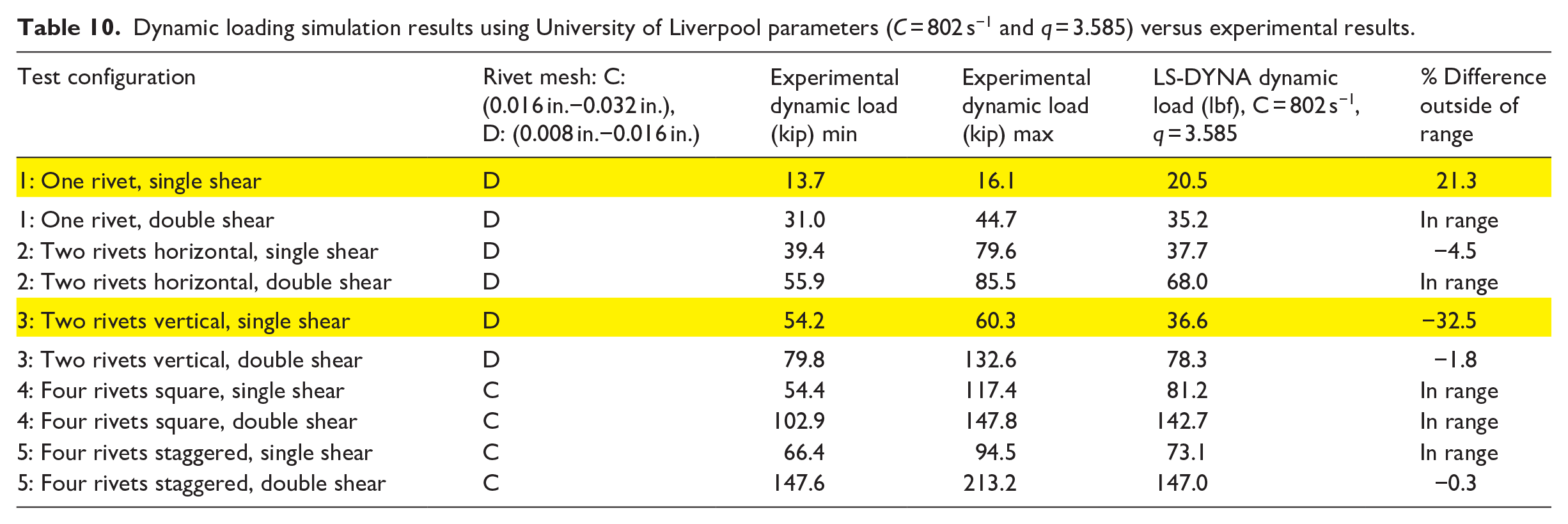
After again setting aside the anomalies from the experimental testing, the University of Liverpool parameters (C = 802 s⁻¹ and q = 3.585) clearly provided the best representation of rivet behavior in shear under high loading rates. In five of the eight analyses, the LS-DYNA output demonstrated ultimate shear strengths within the range of the experimental values. For the other three analyses, the LS-DYNA output predicted ultimate shear strengths within 4.5 percent of the low end of the experimental range. These results are significantly more accurate than the simulation results obtained using the bounding parameters described previously, which under-predicted response by as much as 16.3 percent and over-predicted response by as much as 23.4 percent, respectively. A summary of the testing results using the University of Liverpool parameters is shown in Table 10, with the previously mentioned outlier experimental test results highlighted in yellow. In addition, as demonstrated in Figure 12, load versus time curves simulated within LS-DYNA demonstrated a qualitatively similar shape and time to failure when compared to the experimental data (Rabalais, 2015). Thus, the material and constitutive models exhibited comparable behavior and were considered adequate given the experimentally produced test results.

Table 10.

Dynamic loading simulation results using University of Liverpool parameters (C = 802 s⁻¹ and q = 3.585) versus experimental results.

Test configuration	Rivet mesh: C: (0.016 in.−0.032 in.), D: (0.008 in.−0.016 in.)	Experimental dynamic load (kip) min	Experimental dynamic load (kip) max	LS-DYNA dynamic load (lbf), C = 802 s⁻¹, q = 3.585	% Difference outside of range
1: One rivet, single shear	D	13.7	16.1	20.5	21.3
1: One rivet, double shear	D	31.0	44.7	35.2	In range
2: Two rivets horizontal, single shear	D	39.4	79.6	37.7	−4.5
2: Two rivets horizontal, double shear	D	55.9	85.5	68.0	In range
3: Two rivets vertical, single shear	D	54.2	60.3	36.6	−32.5
3: Two rivets vertical, double shear	D	79.8	132.6	78.3	−1.8
4: Four rivets square, single shear	C	54.4	117.4	81.2	In range
4: Four rivets square, double shear	C	102.9	147.8	142.7	In range
5: Four rivets staggered, single shear	C	66.4	94.5	73.1	In range
5: Four rivets staggered, double shear	C	147.6	213.2	147.0	−0.3

Figure 12.

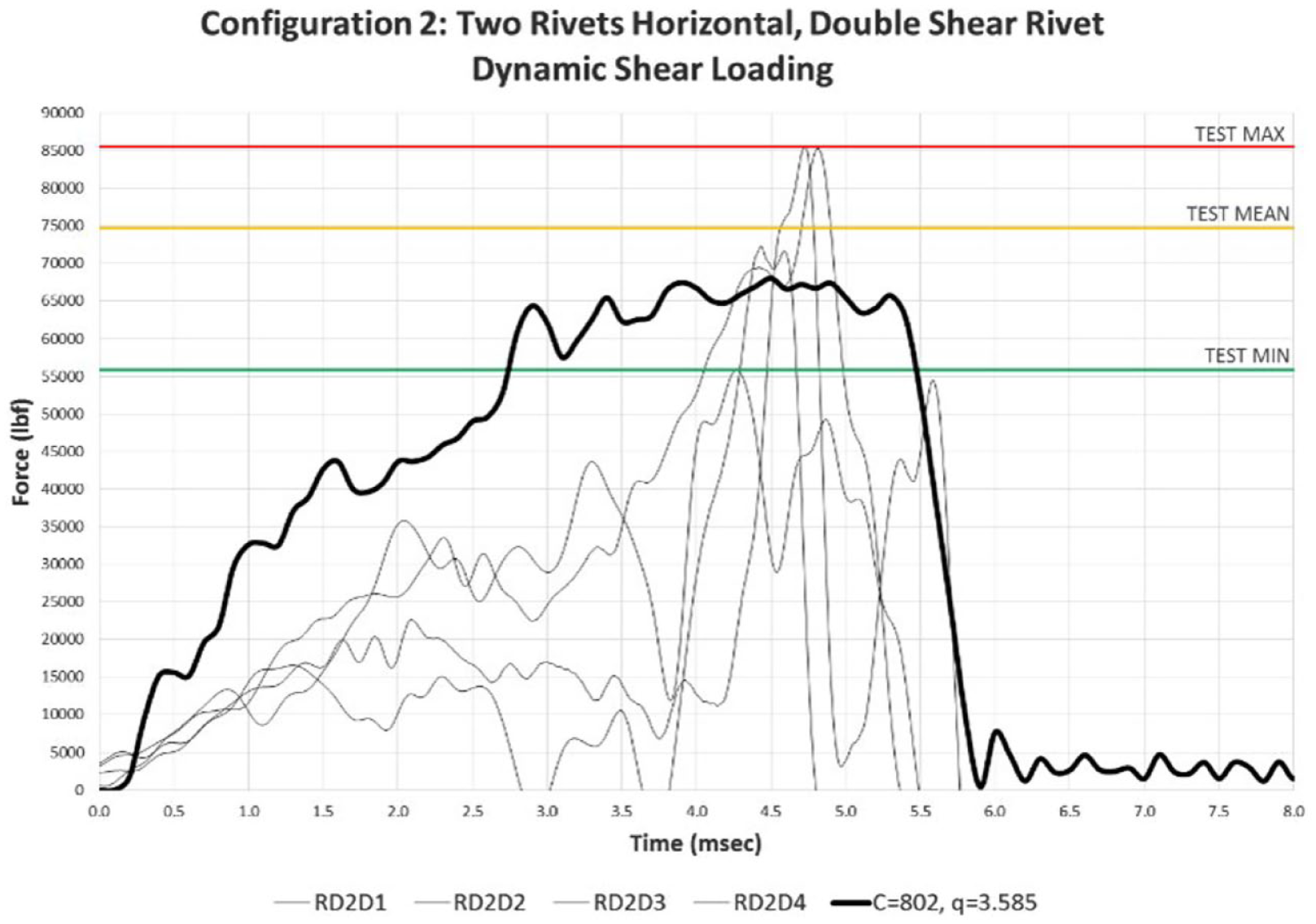
Sample load versus time plot using C = 802 s⁻¹, q = 3.585 (note: test configuration 2: two rivets, horizontal, double shear, in Table 10).

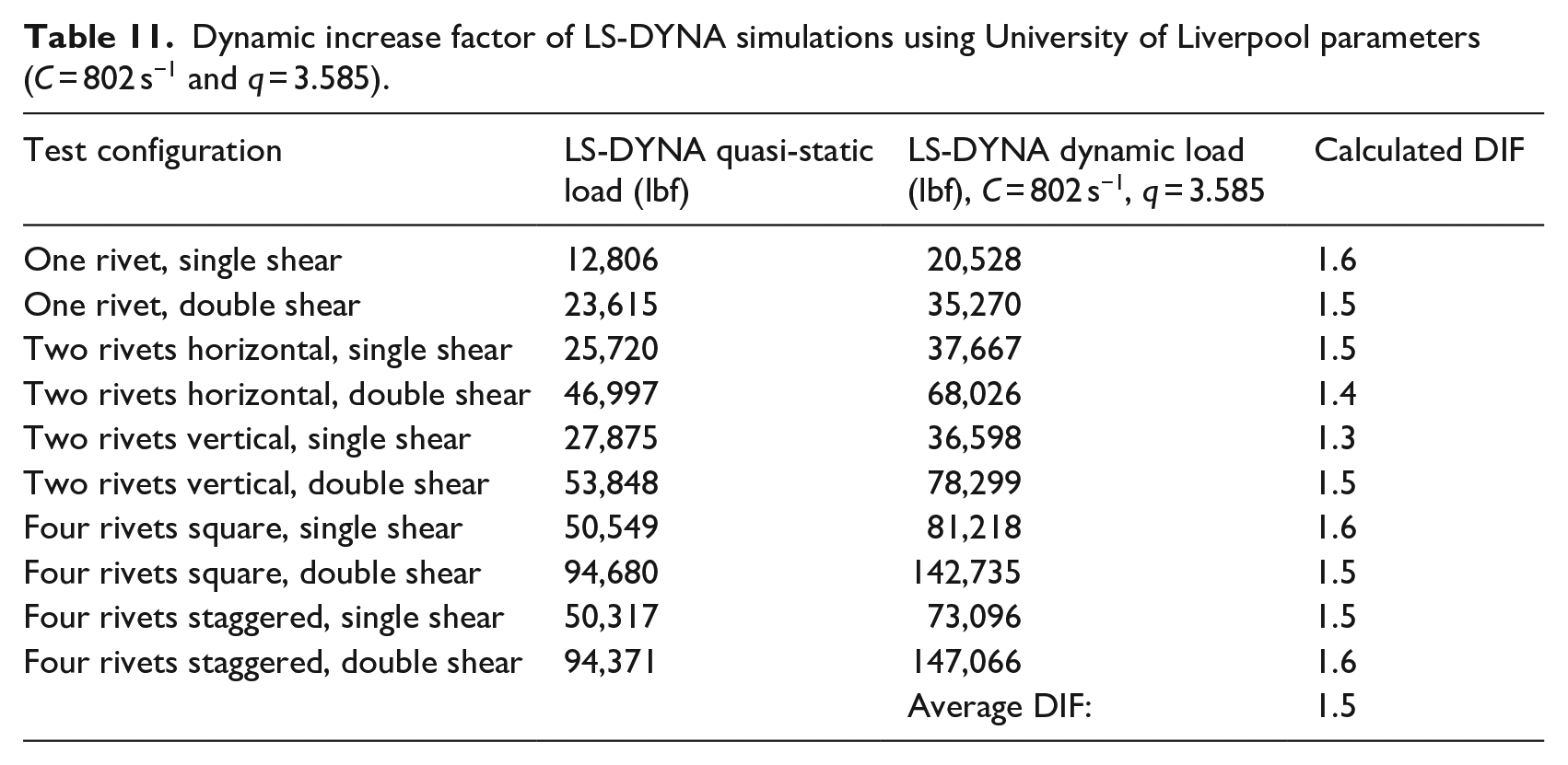
A further look at the LS-DYNA analysis results from the University of Liverpool parameters revealed the calculated dynamic increase factor more closely matches the dynamic increase factor for A502 Grade 2 rivets calculated through the ERDC experimental testing (Rabalais, 2015). As demonstrated in Table 11, the average dynamic increase factor using the University of Liverpool parameters was 1.5, compared to 1.7 from experimental testing (Rabalais, 2015).

Table 11.

Dynamic increase factor of LS-DYNA simulations using University of Liverpool parameters (C = 802 s⁻¹ and q = 3.585).

Test configuration	LS-DYNA quasi-static load (lbf)	LS-DYNA dynamic load (lbf), C = 802 s⁻¹, q = 3.585	Calculated DIF
One rivet, single shear	12,806	20,528	1.6
One rivet, double shear	23,615	35,270	1.5
Two rivets horizontal, single shear	25,720	37,667	1.5
Two rivets horizontal, double shear	46,997	68,026	1.4
Two rivets vertical, single shear	27,875	36,598	1.3
Two rivets vertical, double shear	53,848	78,299	1.5
Four rivets square, single shear	50,549	81,218	1.6
Four rivets square, double shear	94,680	142,735	1.5
Four rivets staggered, single shear	50,317	73,096	1.5
Four rivets staggered, double shear	94,371	147,066	1.6
		Average DIF:	1.5

As described previously, necking should not occur under pure shear. Illustrations of the dynamic loading and eventual failure of the rivets in pure shear are shown in Figures 13 and 14. These illustrations demonstrate Configuration 4 (four rivets square) in double shear. As was consistent in each of the 10 dynamic LS-DYNA simulations, no necking was evident in the fracture of the rivets, providing further confidence in the models.

Figure 13.

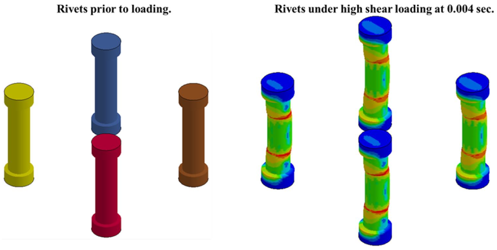
Rivets loaded under high loading rate.

Figure 14.

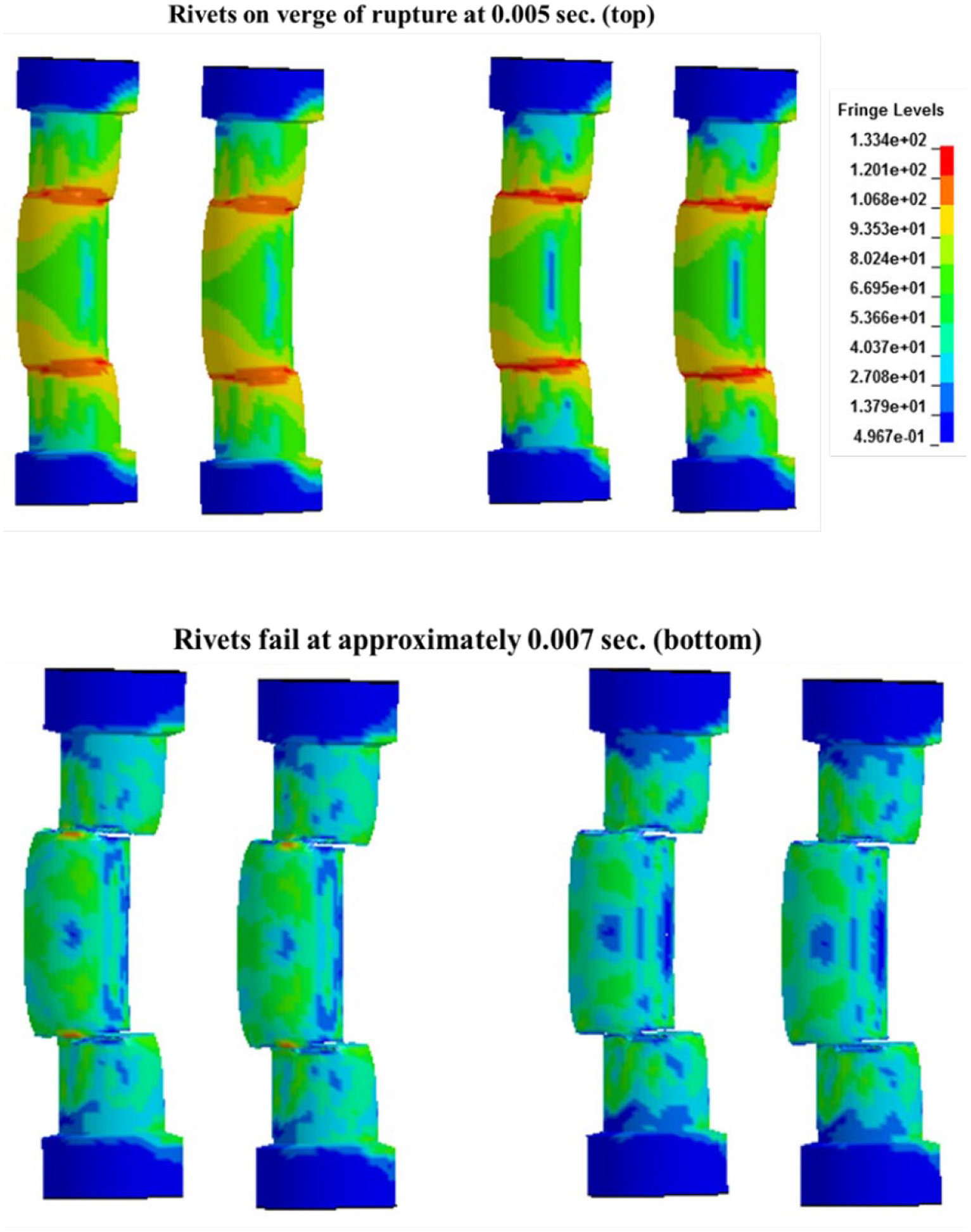
Rivet failure in pure shear under high loading rate.

Conclusion

The first objective of this paper was to provide guidance on modeling rivets using a nonlinear transient dynamic finite element analysis software package. The purpose of this work was to reveal modeling issues that could lead to inaccuracies and shortcomings of the numerical modeling tools. Observations from the model development and simulations give rise to the following conclusions:

A502 Grade 2 rivets can be efficiently and accurately modeled in LS-DYNA and LS-Prepost using three-dimensional, 8-node hexahedra solid elements that utilize the under-integrated constant stress implementation (ELFORM 1) with the Belytschko-Bindeman formulation (HG6) for hourglass control.

The mesh density of a finite element model is critical for both accuracy and computational efficiency (i.e. computing time). In modeling A502 Grade 2 rivets, very fine mesh sizes yielded both accurate ultimate shear strengths and failure results; however, they resulted in significantly longer computational times. Coarser meshes provided accurate ultimate shear stress results with faster computational times but failed to demonstrate reasonable ductility. Mesh sizes in the range of 0.008–0.016-in. provided the most accurate results with respect to rivet ultimate shear strengths and failure results. Given the large computational demand of those simulations, however, this research recommends the use of mesh sizes in the range of 0.016–0.032-in. to model rivets for the best combination of accuracy and efficiency.

The piecewise-linear plasticity model (MAT24) within LS-DYNA provides users with the option of defining a true stress and true strain curve, consisting of up to eight linear segments, to approximate experimental non-linear engineering stress and engineering strain behavior. The input shown in Table 1 for effective plastic strain (in./in.) and corresponding yield stress (ksi) approximates the engineering stress and engineering strain behavior for A502 Grade 2 rivets.

The second objective of this paper was to provide recommendations with respect to modeling strain rate effects for steel rivets. Observations from the model development and simulations lead to the following conclusions:

The Cowper and Symonds constitutive model within the piecewise-linear plasticity model (MAT24) of LS-DYNA provided a simple, efficient, and accurate means of predicting the behavior of A502 Grade 2 rivet connections under high loading rates.

The Cowper and Symonds (1957) parameters (C = 40.4 s⁻¹ and q = 5) derived from subjecting mild steel specimens to relatively small strains in the neighborhood of their yield value provided an upper bound to the behavior of rivets under high loading rates. The Abramowicz and Jones (1986) parameters

(C = 6884 s⁻¹ and q = 3.91) derived from the dynamic axial crushing of mild steel square tubes provided a lower bound to the behavior of rivets under high loading rates. Given the large scatter observed in experimental rivet response, both the upper-bound and the lower-bound parameters are recommended for examination when analyzing riveted suspension panels under blast loads as the difference in the two may affect the failure modes of the steel suspension panels.

With respect to the simulations conducted for this research, the University of Liverpool parameters (C = 802 s⁻¹ and q = 3.585) derived from subjecting mild steel specimens to large strains beyond their yield value provided the most accurate prediction of rivet connection behavior under high loading rates. These parameters are recommended as the sole parameters used in situations where time is limited or in the event where multiple simulations cannot be run.

Footnotes

Acknowledgements

This research project was supported by the U.S. Army Corps of Engineers (USACE) Engineer Research and Development Center (ERDC). Special thanks to Chris Rabalais for his willingness to share experimental test data which was critical to the LS-DYNA modeling. This paper is a portion of a dissertation published by the primary author for partial fulfillment of a Doctor of Philosophy degree from the University of Texas at Austin. Dr. Eric Williamson was the PhD committee chairman.

Declaration of conflicting interests

The author(s) declared no potential conflicts of interest with respect to the research, authorship, and/or publication of this article.

Funding

The author(s) received no financial support for the research, authorship, and/or publication of this article.

ORCID iD

Aaron Thomas Hill

References

Abramowicz

Jones

(1986) Dynamic progressive buckling of circular and square tubes. International Journal of Impact Engineering 4(4): 243–270.

Allison

(2015) E-mail. Fractured Samples (accessed 26 May 2015).

AutoCAD Civil 3D (2013) Computer software. Version G.55.0.1.

Belytschko

Bindeman

(1993) Assumed strain stabilization of the eight node hexahedral element. Computer Methods in Applied Mechanics and Engineering 105(2): 225–260.

Bendigo

Hansen

Rumpf

(1963) Long bolted joints. Journal of the Structural Division, ASCE 89 (ST6).

Collette

Wouters

D’Aniello

, et al. (2016) Impact of the hot-driving process on the strength and ductility of steel rivets. In: Proceedings of Structural Analysis of Historical Constructions - SAHC 2016, Leuven, Belgium. DOI: 10.1201/9781315616995-194.

Cowper

Symonds

(1957) Strain-hardening and strain-rate effects in the impact loading of cantilever beams. Report no. 28. Brown University: Division of Applied Mathematics.

Crane

Rabalais

Chiarito

(2015) Blast loading of steel bridge towers constructed with new and vintage materials. Report. Vicksburg: U.S. Army Research and Development Center.

Erhart

(2011) Review of solid element formulations in LS-DYNA. Available at: http://www.dynamore.de/de/download/papers/forum11/entwicklerforum-2011/erhart.pdf (accessed 5 October 2013).

10.

FHWA (2003) The blue ribbon panel on bridge and tunnel security: Recommendations for Bridge and Tunnel Security. Available at http://www.fhwa.dot.gov/bridge/security/brp.pdf (accessed 10 September 2013).

11.

Forsberg

(2013) Short introduction to LS-DYNA and LS-PrePost. Available at: http://www.solidmechanics.iei.liu.se/Examiners/Courses/Master_Level/TMHL19/intro_lsdyna_lsprepost.pdf (accessed 5 November 2014).

12.

Hallquist

(2006) LS-DYNA Theory Manual. Livermore: Livermore Software Technology Corporation.

13.

Higgins

Ruble

(1955) Structural uses of high-strength bolts. Transactions 120: 1389–398.

14.

Jama

Nurick

Bambach

, et al. (2012) Steel square hollow sections subjected to transverse blast loads. Thin-Walled Structures 53: 109–122.

15.

Jenkins

(2016) Long-Term Trends in Attacks on Public Surface Transportation in Europe and North America. San Jose, California: Mineta Transportation Institute.

16.

Johnson

Cook

(1985) Fracture characteristics of three metals subjected to various strains, strain rates, temperatures and pressures. Engineering Fracture Mechanics 21(1): 31–48.

17.

Kaplan

(1959) Double Shear Tests of High Strength Bolts. Fritz Laboratory Reports.

18.

Kulak

Fisher

Struik

(1987) Guide to Design Criteria for Bolted and Riveted Joints, 2nd edn. Chicago, IL: American Institute of Steel Construction.

19.

Lindeburg

(2003) Civil Engineering Reference Manual for the PE Exam. Belmont, CA: Professional Publications.

20.

Livermore Software Technology Corporation LS-DYNA (2013) Computer software. Version Smp S R7.0.0.

21.

Livermore Software Technology Corporation LS-Prepost (2014) Computer software. Version 4.1.

22.

Livermore Software Technology Corporation (2012) Available at http://ftp.lstc.com/anonymous/outgoing/jday/hourglass.pdf (accessed 10 December 2014).

23.

Lobo

(2007). Methodology for Selection of Material Models for Plastics Impact Simulation. Available at http://www.datapointlabs.com/testpaks/LS-Dyna07/LS-Dyna07_paper.htm (accessed 20 March 2016).

24.

LS-DYNA Support (2014) Contact Modeling in LS-DYNA. Available at: http://www.dynasupport.com/tutorial/ls-dyna-users-guide/contact-modeling-in-ls-dyna (accessed 3 October 2014).

25.

Marais

Tait

Cloete

(2004) Material testing at high strain rate using the split Hopkinson pressure bar. Latin American Journal of Solids and Structures 1: 319–339.

26.

Melosh

(1993) Identifying the characteristics of finite element analysis convergence curves. Finite Elements for Analysis and Design 13(2–3): 105–113.

27.

Mulcahy

(2007) Mackinac bridge workers recall the highs and the lows. . . and tell tall tales. The Building Tradesman Newspaper, 26 October 2007.

28.

Munse

Cox

(1956) The static strength of rivets subjected to combined tension and shear. Bulletin No. 437. Engineering Experiment Station, University of Illinois.

29.

National Consortium for the Study of Terrorism and Responses to Terrorism (START) (2018) Global Terrorism Database [Data file]. Available at: https://www.start.umd.edu/gtd (accessed 3 December 2018).

30.

Paik

Chung

(1999) A basic study on static and dynamic crushing behavior of a stiffened tube. KSAE Transactions 7(1): 219–238.

31.

Rabalais

(2015) Analysis of bolt and rivet structural fasteners subjected to dynamic and quasi-static shear loadings. MS Thesis, Texas A&M University, College Station, TX.

32.

Steinman

Nevill

(1957) Miracle Bridge at Mackinac. Grand Rapids: Eerdmans.

33.

Walker

Ray

Walker

, et al. (2011a) Validation of Numerical Modeling and Analysis of Steel Bridge Towers Subjected to Blast Loadings: Series 1 Report. ERDC/GSL Technical Report 11-11.

34.

Walker

Ray

Walker

, et al. (2011b) Validation of Numerical Modeling and Analysis of Steel Bridge Towers Subjected to Blast Loadings: Series 2 Report. ERDC/GSL Technical Report 11-11.

35.

Walker

Ray

Walker

, et al. (2011c) Validation of Numerical Modeling and Analysis of Steel Bridge Towers Subjected to Blast Loadings: Series 3 Report. ERDC/GSL Technical Report 11-11.

36.

Walker

Ray

Walker

, et al. (2011d) Validation of Numerical Modeling and Analysis of Steel Bridge Towers Subjected to Blast Loadings: Series 4 Report. ERDC/GSL Technical Report 11-11.

37.

Wallaert

Fisher

(1962) Shear Strength of High-Strength Bolts. Fritz Laboratory Reports 1822.

38.

Wilson

Oliver

(1930) Tension Tests of Rivets. Bulletin No. 210, University of Illinois Engineering Experiment Station.

39.

Wilson

Thomas

(1938) Fatigue Tests on Riveted Joints. Bulletin No. 302, University of Illinois Engineering Experiment Station.

40.

Young

Dunbar

(1928) Permissible Stresses on Rivets in Tension. Bulletin No. 8, University of Toronto Faculty of Applied Science and Engineering.